Point Cloud Stacking: A Workflow to Enhance 3D Monitoring Capabilities Using Time-Lapse Cameras


1
RISKNAT Research Group, GEOMODELS Research Institute, Faculty of Earth Sciences, Universitat de Barcelona, 08028 Barcelona, Spain
2
Institute of Applied Geosciences, School of Earth and Environment, University of Leeds, Leeds LS2 9JT, UK
3
Center for Research on the Alpine Environment (CREALP), Sion, CH-1950 Valais, Switzerland
*
Author to whom correspondence should be addressed.
Remote Sens. 2020, 12(8), 1240; https://doi.org/10.3390/rs12081240
Submission received: 25 March 2020
/
Revised: 9 April 2020
/
Accepted: 10 April 2020
/
Published: 13 April 2020
(This article belongs to the Special Issue Advances in Photogrammetry and Remote Sensing: Data Processing and Innovative Applications)
Abstract
:The emerging use of photogrammetric point clouds in three-dimensional (3D) monitoring processes has revealed some constraints with respect to the use of LiDAR point clouds. Oftentimes, point clouds (PC) obtained by time-lapse photogrammetry have lower density and precision, especially when Ground Control Points (GCPs) are not available or the camera system cannot be properly calibrated. This paper presents a new workflow called Point Cloud Stacking (PCStacking) that overcomes these restrictions by making the most of the iterative solutions in both camera position estimation and internal calibration parameters that are obtained during bundle adjustment. The basic principle of the stacking algorithm is straightforward: it computes the median of the Z coordinates of each point for multiple photogrammetric models to give a resulting PC with a greater precision than any of the individual PC. The different models are reconstructed from images taken simultaneously from, at least, five points of view, reducing the systematic errors associated with the photogrammetric reconstruction workflow. The algorithm was tested using both a synthetic point cloud and a real 3D dataset from a rock cliff. The synthetic data were created using mathematical functions that attempt to emulate the photogrammetric models. Real data were obtained by very low-cost photogrammetric systems specially developed for this experiment. Resulting point clouds were improved when applying the algorithm in synthetic and real experiments, e.g., 25th and 75th error percentiles were reduced from 3.2 cm to 1.4 cm in synthetic tests and from 1.5 cm to 0.5 cm in real conditions.
1. Introduction
The acquisition of point clouds (PCs) using photogrammetric techniques for three-dimensional (3D) modelling of natural surfaces has increased significantly in recent years [1,2]. The ease of acquiring images, as well as the low cost of the whole system (devices to take images and processing software) has democratized access to photogrammetric data and ensures greater accessibility compared to LiDAR (Light Detection and Ranging) PCs. Spurred on by this accessibility more and more data are being acquired and consequently more natural surfaces are being reconstructed and investigated [2,3].
Different algorithms have been recently developed for the treatment of LiDAR PCs [4,5,6] and especially TLS (Terrestrial Laser Scanner) data [7,8,9,10,11,12], entailing a wider use of PCs acquired by photogrammetric systems in several geoscience fields [2,3,13]. Examples include: a classification algorithm using a multi-scale dimensionality criterion called “CAractérisation de NUages de POints (CANUPO)” [9]; the geomorphological change detection algorithm “Multi-scale Model to Model Cloud Comparison (M3C2)” [14] and a four-dimensional (4D) workflow for detecting changes in PCs [11] or [15]. Notably, the work by Kromer et al. [11] proposed computing the median distances of a series of point clouds acquired at different time steps and with respect to a fixed reference, extending the M3C2 algorithm [14] to 4D. Kromer et al. [11] and Lague et al. [14] obtained a better level of detection on PC comparison by minimizing point scattering around a central value, they do not improve the PC per se. Although these algorithms were originally developed with the aim of improving results by taking into account the properties and errors of LiDAR datasets, they can be used with PCs captured using different sensors (LiDAR, sonar, etc.); nevertheless, the particular characteristics of photogrammetric data such as non-linear and time-variant errors require the development of new methodologies specifically designed to overcome the constraints of this technique. Interestingly, improving PC quality by stacking multiple low-quality datasets as those generated using time-lapse cameras has not been explored yet.
1.1. Photogrammetry vs. LiDAR 3D Point Cloud Errors
The transformation of digital images into photogrammetric PCs using the technique called Structure from Motion (SfM) consists of estimating the three-dimensional position of points in the space defined from two-dimensional (2D) images [3,16]. Nowadays, both commercial and open-source software products are available for this purpose [17]. In addition to the SfM algorithms, these suites incorporate different tools and utilities to improve the quality of the processing such as the masking of images, the automatic detection of markers, the refinement of camera calibration and the filtering of points based on their quality.
Since the SfM technique is based on iterations of various processes during the bundle adjustment, the obtained PC is a possible solution among many possible results. The quality of the generated PC depends both on the number of homologous points identified and on the quality of the bundle adjustment [18]. For this reason, any repeatability analysis carried out using different images of the same site implies the generation of photogrammetric models with significantly different geometries due to the different random solutions in both camera position estimation and internal calibration parameters. These geometric differences, which can be called geometric errors, will be more or less significant depending on the quality of the homologous points and the bundle adjustment, which depends on the quality of the photographs.
This type of error contrasts strongly with the errors that are obtained in the LiDAR PCs. LiDAR, whose operation is extensively described in Petrie and Toth [19] and Jaboyedoff et al. [6], generates geometrically consistent models; however, due to its operation, the PCs obtained have a random Gaussian noise distributed along all points [11]. This dispersion, called random error, was easily solved and was the theoretical basis of the development of many algorithms for the processing of LiDAR data [14,20].
Several studies have shown that the use of photogrammetric techniques does not result in a particular loss of accuracy with respect to LiDAR PCs [16,21,22,23]. It should be noted, however, that these studies are mostly based on large-scale or detailed laboratory analyses in which hundreds of photographs and numerous control points were used to generate the models. It is well known that the accuracy of LiDAR data depends mainly on the device used to acquire the data. In contrast, the accuracy of the photogrammetric data depends on many other factors such as the camera setup, the weather conditions and the sharpness of the acquired images.
1.2. Landslide Monitoring Using Photogrammetry
The use of digital photogrammetry for landslide monitoring has evolved considerably over the past few years. Photogrammetric monitoring methods can be divided into those using a single camera position plus Digital Image Correlation (DIC) techniques [24] to detect changes between two images captured at different times [25,26], and those that use images taken from different positions (multi-view methods) [27]. One advantage of these photogrammetric techniques is that, in addition to the analysis of current changes, they allow old deformations to be studied by scanning analogue photographs taken before the development of the methodology [28].
Model comparisons and difference calculations can be obtained from: (a) one-dimensional (1D) values resulting from topographic sections extracted from Digital Terrain Models (DTM) [28]; (b) 2D displacements in the image plane obtained using DIC methods [26]; (c) in 3D from the comparison of PCs obtained by SfM techniques [27]; and (d) the 4D analysis based on multi-temporal PC comparisons [29].
As mentioned by Gabrieli et al. [25], it is possible to obtain 3D information of the displacement of a landslide with a single camera, using complex DIC methods and a reference DTM. Even so, several factors, such as the orientation of the deformation and the range and the magnitude of the movement, have a decisive effect on the accuracy of the results. In addition, classical DIC is strongly influenced by changes in illumination [30] and normally assumes that the main deformation field is parallel to the internal camera coordinate system, which is not always the case. Thus, the deformation field should be subsequently orto-rectified using a DTM (e.g., Travelletti et al. [26]).
The use of methods based on multi-view techniques for the study of landslides also carries some limitations, as described in Tannant [31] and Cardenal et al. [27]. These studies can be approached from two different angles. The first consists of obtaining a large number of images from different camera positions to provide algorithms with a large amount of data. The second strategy consists of implementing 4D monitoring by using photogrammetric systems with fixed cameras. In this case, the number of images is limited as it depends directly on the number of cameras installed. These workflows allow the generation of 3D models with a high temporal (sub-daily) frequency, allowing detailed monitoring of deformation, as well as 4D analysis.
The most recent studies in the field of geosciences [29,32] emphasize the importance of two key elements of the SfM process to obtain good quality results. The first is the need to perform lens calibration to obtain the internal parameters of the camera. These parameters, some of which are highly sensitive, allow the elimination of radial and tangential distortion, correcting the deformations of the resulting models. The second element consists of positioning ground control points (GCP) in order to estimate the fit of the models to the real surface. James et al. [33] developed tools to optimize SfM processes by analyzing the parameters that allow better ground control quality. They processed the output of ground control point and point precision analyses using Monte Carlo approaches. These improvements allow the calculation of 3D uncertainty-based topographic change from precision maps. Santise et al. [34] tried to improve the photogrammetric models by reducing the image noise from a three-image merge (see Section 1.3). Additionally, Parente et al. [18] demonstrated an improvement in monitoring quality when a fixed-camera approach was adopted, even with a poor camera calibration procedure. However, there are no algorithms or workflows available to improve the photogrammetric models via the modification of the calculated PCs based on error reduction strategies.
Although several authors have emphasized the importance of using GCP and lens calibration [2,33], in some contexts, such as landslide monitoring, this is impossible due to the unfeasibility of installing targets such as GCP on inaccessible slopes. In addition, obtaining calibration parameters fixed in time is difficult on a high frequency (time-lapse) basis in a fixed area and in remote locations. These limitations, combined with the reduced number of images obtained by fixed camera systems, imply a reduction in the quality of the resulting models compared to those obtained with TLS.
Based on the above, the accuracy and resolution of photogrammetry-derived PCs are strongly controlled not only by internal characteristics (instrument specifications) but also by external considerations (range, number and setup of stations, deformation magnitude, etc.). While TLS is thought to provide a more robust data set compared with SfM, no single technology is universally best suited to all situations because of the wide variety of fieldwork setup and instrumental considerations [35]. On the one hand, the limited number of stations and subsequent occlusions in TLS-derived PCs have been highlighted as one of the main TLS limitations [36]. On the other hand, loss of fine-scale details due to rounding off or over-smoothing of the SfM-derived surfaces on sharp outcrop corners has been observed by several authors (e.g., Wilkinson et al. [35] and Nouwakpo [37]).
Compared to TLS, digital photogrammetry is considered a low-cost landslide monitoring system [2,3,23,38]. In addition, the cost of photographic devices (700 €–3000 €) can be considerably reduced by using very low-cost photographic sensor and lens combinations (50 €), thus producing very low-cost monitoring systems. These systems are based on combinations of photographic microsensors (3.76 × 2.74 mm) and low-quality lenses associated with small microcomputers that are designed to obtain, process and store the images acquired. These systems are designed essentially to operate autonomously and in remote areas [34] (see Section 2.3.2.). These configurations are used because they are easy to obtain, easy to program and can be installed in active areas without concerns about damage due to their low cost. However, the use of these devices implies a lower quality of the photogrammetric models due to the low resolution of the sensor, as well as the poor quality of the lenses. For this reason, when very low-cost photogrammetric systems are used, new methodologies to improve the quality of the photogrammetric models are required, such as the one presented in this article.
1.3. Techniques for Image Stacking (2D)
Using 2D stacking algorithms to enhance digital imagery is a common strategy in several disciplines such as astronomy, computer-vision and microscopy; recent examples of astronomical image processing include successful attempts to increase the signal-to-noise ratio (SNR) [39] and the combination of different wavelengths to de-noise imagery of celestial bodies [40]. Image stacking strategies using photographs taken at different f-stops or with the focus point on different parts of the subject (aka “f-stop stacking” or “focus stacking,” respectively) have also been used to extend the depth of field of the composite images in order to overcome blurriness [41]. In addition, various 2D stacking strategies have been tested to derive high quality imagery from a series of 2D photographs, leading to considerable improvements in photogrammetric models, e.g., when using super-resolution images [42]. On the contrary, stacking 2D images under specific conditions might not always entail noteworthy increases in SNR, as reported by Santise et al. [34].
Similarly, diverse image stacking techniques are commonly employed when using satellite Interferometric Synthetic-Aperture Radar (InSAR) techniques to monitor ground deformation, as recently reported by Selvakumaran et al. [43]. Indeed, atmospheric noise is filtered when using these strategies, leading to a higher SNR and a more accurate DinSAR time series as pointed out by Manconi [30]. In the same way, 2D stacking plays an important role in other fields such as Seismic Data Processing, improving the overall SNR and overall quality of seismic data [44]. Although several publications describing stacking techniques on 2D matrices were found in the literature, no other publications dealing with the improvement of 3D objects (e.g., PCs) were identified during our literature review.
1.4. Aim and Objectives
The aim of this manuscript is to present and validate a workflow to enhance the monitoring capabilities of time-lapse camera systems by stacking individual 3D point clouds generated from Multi View Stereo (MVS) photogrammetry.
The proposed workflow allows the accuracy of the individual PC to be improved by getting the most out of the iterative solutions obtained during the bundle adjustment process, a key step in the MVS photogrammetry workflow. More specifically, bundle adjustment resolves an indeterminate system with a larger number of unknowns than equations (intrinsic and extrinsic camera parameters vs. number of cameras/perspectives respectively), thus, multiple solutions in the form of PCs satisfying these equations are possible. Since the average value in a local coordinate system of the “range” coordinate converges for a large enough size sample (i.e., total number of PCs), a gain in precision can be obtained by stacking and averaging this value on the individual PC, allowing the correction of individual geometric aberrations, as shown below.
The proposed workflow was tested using a synthetic point cloud, created using mathematical functions that attempted to emulate the photogrammetric models, and data collected from a rock cliff located in Puigcercós (Catalonia, NE Spain), using very low-cost photogrammetric systems specially developed for this experiment. This work demonstrates that the proposed workflow is especially well-suited for improving precision when a high temporal sampling procedure can be set up or when low-cost time-lapse camera systems are being used, or both.
2. Materials and Methods
2.1. PCStacking Workflow
2.1.1. Automatic 3D Reconstruction from Time-Lapse Camera Systems
Structure from Motion photogrammetry with multi-view stereo (SfM-MVS) reconstruction was used to generate 3D point clouds from time-lapse camera systems by: (a) Finding correspondence between images through the identification of key features (tie points) in two or more images as homologous points, using a Scale Invariant Feature Transform (SIFT) algorithm [45]. This process is scale, lighting and orientation invariant for all photographs, in order to account for different camera locations and zoom; (b) Estimating the interior and exterior orientation parameters, including the position of each time-lapse system, as well as its orientation and their distortion parameters that satisfy the equations of the “bundle adjustment.” This iterative process consists of minimizing the squared Euclidean distance between the coordinates of each point and its re-projection in each of the iterations, in order to progressively refine the value of each of these parameters. This process was carried out in Agisoft Metashape software (2019 Agisoft). A more detailed description of the SfM-MVS procedure can be seen in Westoby et al. [3]. The SfM workflow results in a sparse PC containing the three-dimensional location of a series of key points in a local coordinate system, together with an estimate of the interior and exterior orientation parameters for each image. This allows calculation of the depth maps of the model in order to reconstruct a dense PC using stereo multi-view algorithms such as PMVS2 (Patch-based MultiView Stereo) [46], CMVS (Clustering Views for MultiView Stereo) [47] and other algorithms integrated in commercial software (e.g., Agisoft Metashape).
2.1.2. Point Cloud Stacking Algorithm
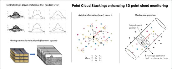
The proposed workflow makes the most of the different solutions generated iteratively during the bundle adjustment and is based, on the one hand, on optimal data collection using time-lapse camera systems and, on the other hand, on an algorithm that generates an enhanced PC from a series of stacked PCs. The proposed method of data collection differs from classic photogrammetry in that, for each of the camera positions, multiple and successive images are captured, in synchrony with the other cameras. This allows the generation of different approximate solutions (Point Clouds) that serve as input data in the PCStacking algorithm. Each individual PC is then stacked and processed in order to generate an enhanced 3D model as the output (Figure 1).
The main steps of the algorithm are (Figure 1): (1) point cloud stacking, (2) local axis transformation and (3) median computation along the normal vector. More specifically, all the individual PCs are stored in a single point cloud (“PC-Stack”) in the first step. Then, a Principal Component Analysis (PCA) is used to transform the global coordinate system to a local coordinate system, so that the third principal component on this orthogonal transformation (rotation and translation) would be defined as the local normal vector. Finally, the algorithm averages the third eigenvalue along the third eigenvector on each point of PC-Stack using the median operator. For practical purposes, this local vector can also be computed with a cylinder of radius r and infinite length in the local normal direction. An extra-dense PC is obtained as a result, where all points have the averaged (median) coordinate for a local subset of points. The overall principle of the proposed algorithm is quite straightforward: point cloud precision can be enhanced by increasing the sample size in order to compensate for systematic errors in a large enough number of datasets, although this does not improve accuracy. The main steps of the Algorithm 1 can be found in the pseudo-code below:
| Algorithm 1 PCStacking is |
| 1 Start |
| 2 get the number of Point Clouds (m) from a designated folder |
| 3 load m Point Clouds into the workspace |
| 4 merge all Point Clouds into a single matrix (PC-Stack) [step 1] |
| 5 input search radius value (r1) |
| 6 for each Point in PC-Stack |
| 7 create a subset1 of PC-Stack inside r1, with coordinates (x,y,z) |
| 8 apply axes transformation (PCA), being normal vector -> Z1 axes [step 2] |
| 9 compute median value of the subset1 along eigen vectors (X, Y, Z) [step 3] |
| 10 end |
| 11 output the mean coordinates of the stacked Point Cloud |
| 12 End |
2.2. Experimental Design (I): Synthetic Test
2.2.1. Synthetic Point Clouds Creation
A synthetic test space formed by PCs that emulate the errors observed in Photogrammetric Point Clouds (Phot-PC) was performed, in order to assess the PCStacking algorithm. In the first instance, a regular perfect surface (without any geometric error) was created using Equation (1). This surface is considered the Reference Point Cloud (Ref-PC):
Then, two different errors are added into the synthetic function, modifying the position of their points in order to simulate the typical errors in photogrammetric data. The first error added is based on a function that keeps the X and Y coordinates but adds a deviation in Z (Equation (2)). This Z deviation is generated using sinusoidal functions because the differences in each point must be related to the previous one. The goal of this process is to generate a geometric error with a solution of continuity avoiding random errors. The values {x,y,z} in Equation (2) correspond to the coordinates of the points in the Ref-PC and the parameters {A,f,d1,d2} are calculated randomly using predefined ranges. That means the synthetic test suite generates a different error (zsin) in each iteration (Figure 2):
The result of Equation (2) is added directly to the Z coordinate in Ref-PC, obtaining a PC with deformations along the Z axis, which can be considered as the geometric error inherent to the photogrammetric models (see Section 1.1). The second error added to the Ref-PC is a random Gaussian distribution error. This error, similar to the one inherent to LiDAR PCs, has little presence in photogrammetric models. However, it is introduced in order to avoid totally regular surfaces. This error is entered into the three coordinates and is defined as ,
and . Finally, the Synthetic Point Cloud (Synt-PC) is obtained from the sum of the Ref-PC coordinates, the geometric deformation obtained by the sinusoidal function (Equation (2)) and the Gaussian scattering errors (Equations (3)–(5)):
The first row of Figure 2 shows the original Ref-PC created with Equation (1) without errors. The first column shows the random functions generated by the sinusoidal function (Equation (2)) and the second column shows the sum of this function with the Ref-PC. The third and fourth columns display cross-sections showing the geometric differences of the resulting PCs with respect to the Ref-PC.
As the PCStacking algorithm needs different simultaneous photogrammetric models to obtain an Enhanced Point Cloud (Enh-PC), 20 random functions were generated, and 20 different Gaussian scattering errors were calculated in order to obtain 20 Synt-PC. This allowed analysis of the performance of the PCStacking algorithm, as well as the sensitivity of the method.
These 20 Synt-PCs emulate the different simultaneous photogrammetric models that would later be generated using real photographs. Figure 3 shows the X and Y cross-sections of five of these Synt-PCs as well as a comparison between two of them using the M3C2 algorithm [14] in CloudCompare software [48]. This comparison was carried out to verify whether or not the differences between different Synt-PCs resembled the differences between two real photogrammetric models (see Section 2.3.3.).
2.2.2. PCStacking Application
After obtaining the 20 Synt-PCs, the following workflow was designed to test the PCStacking method. This involved applying the PCStacking algorithm to the 20 Synt-PCs to obtain the Enh-PCn (n being the number of Synt-PCs considered). The resulting Enh-PCn was then compared with the Ref-PC. The Synt-PCs were introduced into the algorithm in an incremental way, from two to 20 Synt-PCs. Then, each Enh-PCn was compared with the Ref-PC in order to assess the performance of the designed method, as well as its sensitivity to the number of Synt-PCs introduced.
PCStacking test summary:
- -
- Design a Reference PC (Ref-PC)
- -
- Create 20 Synthetic PCs (Synt-PC)
- -
- Application of the PCStacking algorithm: (n -> 2:20)
- o
- Input: n Synthetic PCs (Synt-PC)
- o
- Output: Enhanced PC (Enh-PCn)
- o
- Comparison between the Enhanced PCs (Enh-PCn) and the Reference PC (Ref-PC)
- -
- Analysis of computed differences
The Enh-PCn vs. Ref-PC comparison was carried out using the Point to Mesh algorithm to avoid the influence of statistical averaging of the results using other comparison methods such as the M3C2 algorithm [14]. In this case, the conversion of the Ref-PC into a mesh does not introduce errors because the Ref-PC is a regular surface. For this reason, the distances obtained in the comparison correspond to the real distance between each point of the Enh-PCn and the synthetic surface computed from the Ref-PC. The performance of the developed method was evaluated through the statistical values of the differences between Enh-PCn and Ref-PC, assuming that an improvement means achieving an Enh-PCn more and more similar to the Ref-PC. Thus, the differences obtained in the comparison must tend to zero.
2.2.3. Redundancy Test
Due to the use of random parameters to produce the Synt-PCs, the workflow explained in the previous section was repeated 20 times. Therefore, 400 (20 × 20) different Synt-PCs were calculated to test the PCStacking method, covering a large number of possibilities and providing more consistent results. In each iteration, the standard deviation corresponding to each Enh-PCn vs. Ref-PC comparison was calculated. As this process was repeated 20 times in an iterative way, 20 standard deviation values were obtained for each Enh-PCn vs. Ref-PC comparison. This procedure allowed us to evaluate whether the described method works independently of the random parameters introduced to produce the Synt-PC. This redundancy test was carried out because in some tests the random values of the Synt-PC were too low, which resulted in a Synt-PCs with little error that generated a much improved Enh-PCs. With the generation of 400 Synt-PCs and the computation of the standard deviation of the 400 comparisons (Ref-PC vs. Enh-PC1:2020 times) the median values showed the real range of the PCStacking algorithm.
2.3. Experimental Design (II): 3D Reconstruction of a Rocky Cliff
To observe the performance of the PCStacking algorithm using real data, a test was performed with images obtained by using a photogrammetric system of very low-cost fixed time-lapse cameras on a rock cliff situated in Puigcercós (Catalonia, NE Spain).
2.3.1. Pilot Study Area
The images used for the test were captured from Puigcercós cliff (Catalonia, NE Spain). This rock face (123 m long and 27 m high) is the result of a large rototranslational landslide [49] that occurred at the end of the 19th century [50,51] (Figure 4a). The structure of the area (Figure 4b), together with its high rockfall activity and low risk (due to lack of exposed elements) make it an ideal study area for the development of methodologies such as the TLS point cloud processing methods described by Royán et al., Abellan et al. and Tonini et al. [8,52,53,54].
2.3.2. Field Setup and Data Acquisition
The acquisition of data was carried out using a low-cost photogrammetric system developed ad-hoc for this study. The system consists of five photographic modules and a data transmission module. Each photographic module is composed of a Sony IMX219PQ photographic sensor of 8 megapixels and 1/4" format assembled on a commercial Raspberry Pi Foundation Camera Module V2 board that is characterized by a 3.04-mm focal length lens (29 mm equivalent in 35 mm format) and a maximum aperture of f/2.0. These sensors are controlled by a Raspberry Pi Zero W, a small microcomputer produced by Raspberry Pi Foundation. This computer takes the images and stores and transmits the data to the servers. A solar panel (10 W) and a battery (4500 mAh) are used to power each module. In order to manage the energy source, as well as to carry out the functions of the timer, the commercial board Witty Pi 2 by UUGear is used as a real-time clock and for power management (Figure 5). All these components can be assembled for less than 150 €. Thanks to the remote transmission system based on a 4G WiFi data network and to the solar charging system, the system has very low maintenance costs. The distribution of five photogrammetric modules in five different positions allows the acquisition of daily photogrammetric models of the cliff, inferring a very high temporal frequency of monitoring of rockfalls and deformations.
The quality of the point clouds produced by this low-cost system is theoretically lower than that obtained using commercial cameras, due to the size of the sensor, the low resolution and the quality of the lens. Consequently, the resulting photogrammetric models are not high quality. This system is thus ideal as a case study to monitor the performance of the PCStacking method and to evaluate its ability to generate higher quality photogrammetric models.
Since there is no ideal surface of the terrain that corresponds to the Ref-PC in the synthetic test, the algorithm was tested by comparing the two models acquired on consecutive days (February 25 and 26, 2019) from an area without any activity. Due to the non-activity and therefore the non-existence of movement, we assume that the difference between the models must be zero.
2.3.3. Point Cloud Reconstruction
The system developed on Puigcercós was configured to capture 15 images in the same photo burst synchronized in the five installed cameras. From these 15 photographs captured by each camera, 15 different photogrammetric models of the same moment in time were reconstructed using Agisoft Metashape (2019 Agisoft). To improve the software’s calculation process, different tools such as zone masking, cutting out working areas and optimizing camera positions were used. The results were always obtained at the highest quality, both in the calculation of homologous points and the dense point cloud (PC).
Due to the large size of the rockface and the requirement to work in an area without deformation, we have carried out the test in a specific zone. This truncated rectangle has a size of 12.5 m × 10 m and an area of approximately 100 m2. The computational cost to perform the entire process for a given radius in this small area is around 60 minutes to generate the 3D models with Agisoft Metashape and 70 minutes to apply the PCStacking algorithm. These times have been achieved with a commercial medium-high performance equipment (Intel(R) Core(TM) i9—7900X up to 4.30 GHz, 64GB RAM and NVIDIA GeForce GTX 1080 Ti). The raw point clouds obtained by the Metashape software are composed by approximately 150,000 points.
As the test was carried out on two consecutive days, a total of 30 Photogrammetric Point Clouds (Photo-PC) were generated. The calculated models were aligned and scaled with a reference LiDAR to produce metric values for comparison. Figure 6a shows the X and Y cross-sections of four Photo-PCs. It demonstrates the correct alignment of the models but shows clearly different surfaces due to the poor quality of the acquisition system.
3. Results
3.1. Synthetic Test
The histograms of the differences between the Enh-PCn and the Ref-PC (Figure 7a) provide a quantitative assessment of the improvement achieved with the PCStacking algorithm. The increase in the number of input models (Synt-PCs) resulted in a better fit between Enh-PCn and Ref-PC.
The boxplot in Figure 7b illustrates the distribution of the differences calculated from the comparisons between Enh-PCn vs. Ref-PC. The boxplot depicts a decrease in the errors when more inputs were used. The 25th and 75th percentiles progressively reduced to 50% after using 18 models. Specifically, the percentiles were progressively reduced from ±3.2 cm to ±1.4 cm after using the PCStacking algorithm with 18 models. Likewise, the minimums and maximums shown in the boxplot also showed a reduction close to 50%. The comparisons between Enh-PCn vs. Ref-PC in the redundancy test (Figure 8a) reveal a considerable reduction of the standard deviation when increasing the number of models introduced. The average standard deviations of the comparisons of all iterations decreased from 4.9 cm to 1.8 cm when 20 PC were used.
The quartile bars (Figure 7b and Figure 8a) demonstrate non-constant values because in some iterations the Synt-PCs may have much more error than in others. As an example, in Figure 7b, the 75th percentile bar belonging to the input of 16 Synt-PCs is larger (1.4 cm) than the one belonging to the input of 14 Synt-PCs (1.3 cm). This random distribution of error is the main reason for carrying out the iterative test.
One effect of using the PCStacking method is that the result obtained (Enh-PCn) accumulates all the points of the different Synt-PCs used, producing both a more accurate and denser Enh-PC. The plot in Figure 8b depicts the number of points available to average the Z coordinate, which depends on the number of Synt-PCs used as input data and on the search radius defined. This value is a great indicator of when the algorithm has enough input points to compute the new Z coordinate.
Using this parameter as a filter, those points that were averaged using a smaller number of points were removed from the Enh-PC. For this research, all points in the Enh-PC that were averaged using less than as many points as Synt-PCs introduced, were removed. In this way, this filter easily allows the removal of points in some Enh-PC that are not generally in all Synt-PCs, such that unrepresentative points produced during the reconstruction of the model are removed.
3.2. 3D Reconstruction on a Rocky Cliff
The process for evaluating the algorithm using real images taken on 25th and 26th February 2019 involved: (a) Calculation of the Enh-PCn=2:15 from the February 25th PCs; (b) Calculation of the Enh-PCn=2:15 from the February 26th PCs; (c) Point to mesh comparison (in CloudCompare) between a February 25th Photo-PC and a February 26th Photo-PC without applying any enhancement algorithm; and (d) Point to mesh comparison (in CloudComapre) between all Enh-PC(2:15)25 feb vs. Enh-PC(2:15)26 feb. The outputs from these comparisons are the distances in metric values existing between the two models studied. Given that between 25th and 26th February 2019 there was no change in the analyzed cliff, the expected difference in an ideal case must be zero.
The results obtained are shown in Figure 9, which is analogous to Figure 7. The histogram of the values obtained in the comparison (25th February vs. 26th February) (Figure 9a) demonstrates that the precision of the values increases when more models are added to the algorithm (the differences tend to zero). Moreover, Figure 9b shows a decrease in the 25th and 75th percentiles of almost 70%. Values decreased from ±1.5 cm for a simple comparison to ±0.5 cm when comparing the Enh-PC1525 feb vs. Enh-PC1526 feb.
Figure 10 depicts the sensitivity of the algorithm from the input parameters of the code. The plot in Figure 10a shows the standard deviation obtained in the comparisons made by M3C2 [14] between Enh-PCn25 feb and Enh-PCn26 feb. Each plotted line represents different parameters in the search radius (r) of the PCStacking algorithm (Section 2.1 and Figure 1). Note that for the smaller radius (r = 0.1 cm) the algorithm does not produce any improvement, because as in the synthetic test (Figure 8b), the small search radius does not provide enough points to average the Z coordinate in the direction of the normal.
When the search radius is larger the algorithm has more points to average, resulting in a decrease in the standard deviation of the comparisons. The images in Figure 10b show the comparisons using the M3C2 algorithm between Enh-PC1525 feb and Enh-PC1526 feb for the different search radii described.
Since the proposed algorithm involves averaging the Z coordinate along the normal axis at each point, obtaining the normals at each point in the correct way is critical. As discussed in Lague et al. [14], the roughness of the surface makes the calculation of normals dependent on the scale at which it is performed. Thus, calculating normals using inappropriate scales means that the averaging is not done in the right direction. Consequently, the efficiency of the algorithm decreases considerably.
In the case of the Synth-PC the normals were calculated using the CloudCompare software. However, for the real case of the Puigcercós Cliff, the normals were computed automatically using Agisoft Metashape software (2019 Agisoft) (see Section 4. Discussion).
4. Discussion
4.1. Synthetic Test vs. Real Data
The cross-sections obtained from the synthetic point clouds (Synt-PCs) (Figure 3a) and real photogrammetric models (Photo-PC) (Figure 7a) are very similar. Likewise, the random distribution of the error obtained in a comparison of two Synt-PCs (Figure 3b) is similar to that obtained from real data (Photo-PC) (Figure 6b). The use of random parameters in the sinusoidal function allows the generation of different PCs with errors that are geometrically consistent in each iteration. This is important because in the reconstruction of models obtained using low-cost photogrammetric systems, surfaces with different geometries are always generated even though the input photographs are captured at the same time. The result of using the described functions (Equations (1) and (2)) together with the random parameters (Equations (3)–(5)) generated synthetic PCs with a similar pattern to that of photogrammetric models.
Despite the above mentioned observations, the comparison between two Synth-PCs using the M3C2 algorithm [14] (Figure 3b) depicts some repeatability in the distribution of the differences, while the pattern of the comparison between two Photo-PCs (Figure 6b) is absolutely random. This is because Synth-PCs were created by the sinusoidal function (Equation (2)), which is periodic. Even so, we believe that this conceptual dissimilarity in the distribution of the differences does not affect the PCStacking method trials proposed in this paper.
To sum up, the synthetic study suite designed to test the PCStacking algorithm worked well and the generated PCs are comparable to PCs obtained from low-cost photogrammetric models. Thus, this methodology based on the generation of synthetic functions can be extrapolated to the synthetic study of different PC improvement algorithms.
4.2. The PCStacking Method
The results of the assessment of the PCStacking workflow reveal a significant improvement in the precision of the enhanced point clouds. This advance was observed with both synthetic and photogrammetric PCs. In the synthetic case the initial error of the comparison was larger (±3.2 cm) and the reduction occurred more progressively while introducing a greater number of Synt-PCs to the algorithm, reaching ±1.4 cm in the Enh-PC18 comparison (Figure 7). In contrast, real photogrammetric models had a smaller comparison error that ranged from ±1.5 cm to ±0.5 cm when 15 PCs were used. In this case, 50% reduction in error was achieved when using only five PCs (Figure 9). This is because: (a) the synthetic PCs were designed with a higher geometric error with a distribution dependent on random parameters (see Equation (2)); and (b) the errors in the real photogrammetric PCs are not homogeneous and tend to be concentrated in areas where the software has more difficulty identifying homologous points. Consequently, synthetic data has larger and more distributed errors, thus, the algorithm needs more input point clouds to reduce the error. Even so, the algorithm succeeded in reducing the errors in both the synthetic test and the real case, and the number of PCs used was sufficient to stabilize the error reduction.
Concerning data acquisition, the application of the algorithm using only one image per camera position (classic capture scheme), instead of a set of images as in this study, would reduce its efficiency considerably. The use of different simultaneous images captured in the same burst means that each model is built on the basis of a totally different point identification process and bundle adjustment. This is because the intrinsic errors of the photographic sensors will always generate differences between the images, despite the short time between shots. Consequently, SfM algorithms produce different geometries generating slightly different models. The averaging of these differences through the PCStacking algorithm improves the precision of the PCs obtained from images captured using low-cost systems.
The results of the redundancy test applied to Synt-PCs reveal that the developed code is robust. The goal of this test is to eliminate any possibility of associating the improvement with the use of low random values for the generation of the Synt-PCs. As shown in Figure 8a the standard deviation of the 20 iterations performed progressively decreased as the number of input models increased. The differences in the error bars are related to the randomness of the parameters contemplated in Equation (2) to introduce the random error to the Synt-PCs. Thus, some iterations produce Synt-PC with errors greater than others. This results in point averaging between point clouds with greater dispersion, thus augmenting the error in the comparison Enh-PCn vs. Ref-PC.
The considerable increase in the number of averaged points shown in Figure 8b is due to two key parameters: (1) the number of input PCs and (2) the PCStacking search radius. Therefore, these two parameters control the quality of the result (Figure 10). For this reason, in a real situation, a sensitivity study to determine the parameters that would improve the results is required.
4.3. Current Limits and Margins for Improvement
As shown in Figure 7, Figure 8 and Figure 9, the improvement obtained by the application of the PCStacking method was not linear. In addition, Figure 10a reveals that a sensitivity study of the parameters used is required because, depending on the point density of the input data, the algorithm will start working optimally from a certain search radius. The use of a very large search radius may end up involving excessive smoothing of the Z coordinate. However, the use of a very small search radius will not provide enough information for the PCStacking algorithm to perform point averaging.
The reduction in error (Figure 10a) observed when using a 0.1 cm radius (extremely small) was due to the effect of the densification of the PCStacking algorithm and the averaging of the M3C2 algorithm. In our work, the PCStacking algorithm, with a radius of 0.1 cm, did not average any value because the density of points was too low to include more than one point. Thus, the Enh-PC obtained can be considered the same as if all the input Photo-PCs had been merged without any processing. Since the search radius of the M3C2 for the comparison was the same for all analyses (1 cm), the use of the M3C2 resulted in a reduction in the error as more input Photo-PC were introduced. If the PCStacking algorithm did not have the property of densifying the PC for the 0.1 cm search radius, there would have been no improvement. In order to identify the improvements produced by the PCStacking algorithm, the comparisons between Enh-PCs and Ref-PC in the synthetic test, and between Enh-PCn25 feb and Enh-PCn26 feb in the real case test, were calculated using the Point to Mesh comparison algorithm. Since the application of this algorithm does not produce any improvement by itself, the error reduction shown in Figure 4 and Figure 9 can be associated with the PCStacking algorithm. On the other hand, when a real representation of the distribution of differences between two PCs was needed (Figure 3, Figure 8 and Figure 10), the M3C2 algorithm was used, since this allows better visualization of the results as well as discrimination between positive and negative values of the differences obtained.
Another important consideration before applying the method is the correct determination of the normals for each point. As cited in Lague et al. [14], miscalculation of normals will result in poor adjustment of the method. Since the normals must be calculated based on a search radius, taking into account the roughness of each surface, it is necessary to find the best fit between both the method and the radius to obtain an optimal result with the PCStacking algorithm. However, the normals calculated directly by the digital photogrammetry software are sufficiently well-computed to allow the PCStacking algorithm to work properly.
Although the results presented show an interesting improvement in the field of point clouds, due to the differences in the errors of the photogrammetric models with respect to the LiDAR data explained in the introduction, the efficiency of the PCStacking algorithm will not be equivalent with the LiDAR data. Even so, the algorithm has not been tested with other acquisition systems. Thus, the performance of the algorithm in point clouds obtained with other technologies has not been verified yet. If the proper computation of the normals cannot be guaranteed, the PCStacking method can be applied by modifying part of the algorithm. Instead of averaging only the Z coordinate in the direction of the normal, it will be necessary to average all the coordinates {x,y,z} in the direction of the respective normals. In this case, exploratory tests showed that the method also produced better PCs but with greater surface smoothness.
Another discussion point is the computational cost of applying the algorithm. Digital photogrammetry software generates, at its highest quality, very dense PCs that easily exceed millions of points. Because the PCStacking algorithm is based on the introduction (and accumulation) of different PCs, the workspaces can easily exceed tens of millions of points. Since Z-coordinate averaging is done point-to-point, the computational cost is high. Nevertheless, the PCStacking algorithm can also be used in low performance computers by simply subsampling the original PCs. Therefore, a necessary improvement of the method will involve optimizing the calculation. This optimization could be achieved using dedicated PC library methods that significantly speed up the process as well as the use of PC fractionation methods.
5. Conclusions
This article presents a workflow to increase the precision in the comparison of PCs obtained through Multi-View Stereo photogrammetry. This method, called Point Cloud Stacking (PCStacking), refers to the process of taking photographs, as well as the data processing and post-processing of the information to generate enhanced PCs. This paper describes the application of the method using both synthetic PCs specially developed to emulate photogrammetric models and a real case study, with photogrammetric PCs obtained using a very low-cost time-lapse camera system. The results showed a reduction of more than 50% of the error, increasing the precision in both experiments, and validating the proposed approach under different conditions. In more detail, the 25th and 75th percentiles were progressively reduced with both the synthetic data and the actual photogrammetric models from ±3.2 cm to ±1.4 cm, and from ±1.5 cm to ±0.5 cm respectively. The resulting enhancement means that relatively low-cost strategies could be used in place of more expensive systems, but the proposed algorithm can also be used to repeat TLS scenarios in order to increase the signal-to-noise ratio. The proposed approach might constitute a step forward for high precision monitoring of both natural processes (landslides, glaciers, riverbeds, erosion, etc.) and man-made scenarios (structural monitoring of buildings, tunnels, beams, dams, etc.) using low-cost time-lapse camera systems.
Author Contributions
Algorithm conceptualization and methodology: X.B. and A.A.; software: X.B.; formal analysis: X.B., A.A. and M.G., investigation: X.B., A.A. and M.G., validation: X.B., A.A. and M.G. writing—original draft preparation, X.B.; writing—review and editing A.A. and M.G.; visualization: X.B.; supervision, A.A. and M.G. All authors have read and agreed to the published version of the manuscript.
Funding
The presented study was supported by the PROMONTEC Project (CGL2017-84720-R) funded by the Ministry of Science, Innovation and Universities (MICINN-FEDER). The first author (X. Blanch) was supported by an APIF grant funded by the University of Barcelona and the second author (A. Abellán) was supported by the European Union’s Horizon 2020 research and innovation programme under a Marie Skłodowska-Curie fellowship (grant agreement no. 705215).
Acknowledgments
The authors thank the ORIGENS UNESCO Global Geopark for granting permission to work in Puigcercós rock cliff and the reviewers and the editor for the valuable comments and suggestions that contributed to the improvement of the present manuscript.
Conflicts of Interest
The authors declare no conflict of interest.
References
- Dewez, T.J.B.; Rohmer, J.; Regard, V.; Cnudde, C. Probabilistic coastal cliff collapse hazard from repeated terrestrial laser surveys: Case study from Mesnil Val (Normandy, northern France). J. Coast. Res. 2016, 65, 702–707. [Google Scholar] [CrossRef]
- Eltner, A.; Kaiser, A.; Castillo, C.; Rock, G.; Neugirg, F.; Abellán, A. Image-based surface reconstruction in geomorphometry-merits, limits and developments. Earth Surf. Dyn. 2016, 4, 359–389. [Google Scholar] [CrossRef] [Green Version]
- Westoby, M.J.; Brasington, J.; Glasser, N.F.; Hambrey, M.J.; Reynolds, J.M. “Structure-from-Motion” photogrammetry: A low-cost, effective tool for geoscience applications. Geomorphology 2012, 179, 300–314. [Google Scholar] [CrossRef] [Green Version]
- Riquelme, A.J.; Abellán, A.; Tomás, R.; Jaboyedoff, M. A new approach for semi-automatic rock mass joints recognition from 3D point clouds. Comput. Geosci. 2014, 68, 38–52. [Google Scholar] [CrossRef] [Green Version]
- Derron, M.H.; Jaboyedoff, M. LIDAR and DEM techniques for landslides monitoring and characterization. Nat. Hazards Earth Syst. Sci. 2010, 10, 1877–1879. [Google Scholar] [CrossRef]
- Jaboyedoff, M.; Oppikofer, T.; Abellán, A.; Derron, M.H.; Loye, A.; Metzger, R.; Pedrazzini, A. Use of LIDAR in landslide investigations: A review. Nat. Hazards 2012, 61, 5–28. [Google Scholar] [CrossRef] [Green Version]
- García-Sellés, D.; Falivene, O.; Arbués, P.; Gratacos, O.; Tavani, S.; Muñoz, J.A. Supervised identification and reconstruction of near-planar geological surfaces from terrestrial laser scanning. Comput. Geosci. 2011, 37, 1584–1594. [Google Scholar] [CrossRef]
- Royán, M.J.; Abellán, A.; Jaboyedoff, M.; Vilaplana, J.M.; Calvet, J. Spatio-temporal analysis of rockfall pre-failure deformation using Terrestrial LiDAR. Landslides 2014, 11, 697–709. [Google Scholar] [CrossRef]
- Brodu, N.; Lague, D. 3D terrestrial lidar data classification of complex natural scenes using a multi-scale dimensionality criterion: Applications in geomorphology. ISPRS J. Photogramm. Remote Sens. 2012, 68, 121–134. [Google Scholar] [CrossRef] [Green Version]
- Abellán, A.; Vilaplana, J.M.; Calvet, J.; García-Sellés, D.; Asensio, E. Rockfall monitoring by Terrestrial Laser Scanning—Case study of the basaltic rock face at Castellfollit de la Roca (Catalonia, Spain). Nat. Hazards Earth Syst. Sci. 2011, 11, 829–841. [Google Scholar] [CrossRef] [Green Version]
- Kromer, R.A.; Abellán, A.; Hutchinson, D.J.; Lato, M.; Edwards, T.; Jaboyedoff, M. A 4D filtering and calibration technique for small-scale point cloud change detection with a terrestrial laser scanner. Remote Sens. 2015, 7, 13029–13058. [Google Scholar] [CrossRef] [Green Version]
- Jaboyedoff, M.; Demers, D.; Locat, J.; Locat, A.; Locat, P.; Oppikofer, T.; Robitaille, D.; Turmel, D. Use of terrestrial laser scanning for the characterization of retrogressive landslides in sensitive clay and rotational landslides in river banks. Can. Geotech. J. 2009, 46, 1379–1390. [Google Scholar] [CrossRef]
- Smith, M.W.; Carrivick, J.L.; Quincey, D.J. Structure from motion photogrammetry in physical geography. Prog. Phys. Geogr. 2015, 40, 247–275. [Google Scholar] [CrossRef]
- Lague, D.; Brodu, N.; Leroux, J. Accurate 3D comparison of complex topography with terrestrial laser scanner: Application to the Rangitikei canyon (N-Z). ISPRS J. Photogramm. Remote Sens. 2013, 82, 10–26. [Google Scholar] [CrossRef] [Green Version]
- Williams, J.G.; Rosser, N.J.; Hardy, R.J.; Brain, M.J.; Afana, A.A. Optimising 4-D surface change detection: An approach for capturing rockfall magnitude-frequency. Earth Surf. Dyn. 2018, 6, 101–119. [Google Scholar] [CrossRef] [Green Version]
- James, M.R.; Robson, S. Straightforward reconstruction of 3D surfaces and topography with a camera: Accuracy and geoscience application. J. Geophys. Res. Earth Surf. 2012, 117, 1–17. [Google Scholar] [CrossRef] [Green Version]
- Eltner, A.; Schneider, D. Analysis of Different Methods for 3D Reconstruction of Natural Surfaces from Parallel-Axes UAV Images. Photogramm. Rec. 2015, 30, 279–299. [Google Scholar] [CrossRef]
- Parente, L.; Chandler, J.H.; Dixon, N. Optimising the quality of an SfM-MVS slope monitoring system using fixed cameras. Photogramm. Rec. 2019, 34, 408–427. [Google Scholar] [CrossRef]
- Petrie, G.; Toth, C. Introduction to Laser Ranging, Profiling, and Scanning. In Topographic Laser Ranging and Scanning; Shan, J., Toth, C.K., Eds.; CRC Press/Taylor & Francis: London, UK, 2008; pp. 1–28. [Google Scholar]
- Abellán, A.; Jaboyedoff, M.; Oppikofer, T.; Vilaplana, J.M. Detection of millimetric deformation using a terrestrial laser scanner: Experiment and application to a rockfall event. Nat. Hazards Earth Syst. Sci. 2009, 9, 365–372. [Google Scholar] [CrossRef] [Green Version]
- Kaiser, A.; Neugirg, F.; Rock, G.; Müller, C.; Haas, F.; Ries, J.; Schmidt, J. Small-scale surface reconstruction and volume calculation of soil erosion in complex moroccan Gully morphology using structure from motion. Remote Sens. 2014, 6, 7050–7080. [Google Scholar] [CrossRef] [Green Version]
- Castillo, C.; Pérez, R.; James, M.R.; Quinton, J.N.; Taguas, E.V.; Gómez, J.A. Comparing the accuracy of several field methods for measuring gully erosion. Soil Sci. Soc. Am. J. 2012, 76, 1319–1332. [Google Scholar] [CrossRef] [Green Version]
- Javernick, L.; Brasington, J.; Caruso, B. Modeling the topography of shallow braided rivers using Structure-from-Motion photogrammetry. Geomorphology 2014, 213, 166–182. [Google Scholar] [CrossRef]
- Pan, B. Digital image correlation for surface deformation measurement: Historical developments, recent advances and future goals. Meas. Sci. Technol. 2018, 29, 1–32. [Google Scholar] [CrossRef]
- Gabrieli, F.; Corain, L.; Vettore, L. A low-cost landslide displacement activity assessment from time-lapse photogrammetry and rainfall data: Application to the Tessina landslide site. Geomorphology 2016, 269, 56–74. [Google Scholar] [CrossRef]
- Travelletti, J.; Delacourt, C.; Allemand, P.; Malet, J.P.; Schmittbuhl, J.; Toussaint, R.; Bastard, M. Correlation of multi-temporal ground-based optical images for landslide monitoring: Application, potential and limitations. ISPRS J. Photogramm. Remote Sens. 2012, 70, 39–55. [Google Scholar] [CrossRef]
- Stumpf, A.; Malet, J.P.; Allemand, P.; Pierrot-Deseilligny, M.; Skupinski, G. Ground-based multi-view photogrammetry for the monitoring of landslide deformation and erosion. Geomorphology 2015, 231, 130–145. [Google Scholar] [CrossRef]
- Cardenal, J.; Mata, E.; Delgado, J.; Hernandez, M.A.; Gonzalez, A. Close Range Digital Photogrammetry Techniques Applied To. Int. Arch. Photogramm. Remote Sens. Spat. Inf. Sci. 2008, XXXVI, 235–240. [Google Scholar]
- Kromer, R.; Walton, G.; Gray, B.; Lato, M.; Group, R. Development and Optimization of an Automated Fixed-Location Time Lapse Photogrammetric Rock Slope Monitoring System. Remote Sens. 2019, 11, 1890. [Google Scholar] [CrossRef] [Green Version]
- Manconi, A.; Kourkouli, P.; Caduff, R.; Strozzi, T.; Loew, S. Monitoring surface deformation over a failing rock slope with the ESA sentinels: Insights from Moosfluh instability, Swiss Alps. Remote Sens. 2018, 10, 672. [Google Scholar] [CrossRef] [Green Version]
- Tannant, D. Review of Photogrammetry-Based Techniques for Characterization and Hazard Assessment of Rock Faces. Int. J. Geohazards Environ. 2015, 1, 76–87. [Google Scholar] [CrossRef] [Green Version]
- Eltner, A.; Kaiser, A.; Abellan, A.; Schindewolf, M. Time lapse structure-from-motion photogrammetry for continuous geomorphic monitoring. Earth Surf. Process. Landf. 2017, 42, 2240–2253. [Google Scholar] [CrossRef]
- James, M.R.; Robson, S.; d’Oleire-Oltmanns, S.; Niethammer, U. Optimising UAV topographic surveys processed with structure-from-motion: Ground control quality, quantity and bundle adjustment. Geomorphology 2017, 280, 51–66. [Google Scholar] [CrossRef] [Green Version]
- Santise, M.; Thoeni, K.; Roncella, R.; Sloan, S.W.; Giacomini, A. Preliminary tests of a new low-cost photogrammetric system. Int. Arch. Photogramm. Remote Sens. Spat. Inf. Sci. -ISPRS Arch. 2017, 42, 229–236. [Google Scholar] [CrossRef] [Green Version]
- Wilkinson, M.W.; Jones, R.R.; Woods, C.E.; Gilment, S.R.; McCaffrey, K.J.W.; Kokkalas, S.; Long, J.J. A comparison of terrestrial laser scanning and structure-frommotion photogrammetry as methods for digital outcrop acquisition. Geosphere 2016, 12, 1865–1880. [Google Scholar] [CrossRef] [Green Version]
- Sturzenegger, M.; Yan, M.; Stead, D.; Elmo, D. Application and limitations of ground-based laser scanning in rock slope characterization. In Proceedings of the 1st Canada—U.S. Rock Mechanics Symposium, Simon Fraser University, Burnaby, BC, Canada, 27–31 May 2007; Volume 1, pp. 29–36. [Google Scholar]
- Nouwakpo, S.K.; Weltz, M.A.; McGwire, K. Assessing the performance of structure-from-motion photogrammetry and terrestrial LiDAR for reconstructing soil surface microtopography of naturally vegetated plots. Earth Surf. Process. Landf. 2016, 41, 308–322. [Google Scholar] [CrossRef]
- Verma, A.K.; Bourke, M.C. A method based on structure-from-motion photogrammetry to generate sub-millimetre-resolution digital elevation models for investigating rock breakdown features. Earth Surf. Dyn. 2019, 7, 45–66. [Google Scholar] [CrossRef] [Green Version]
- Bin, W.; Hai-bin, Z.; Bin, L. Detection of Faint Asteroids Based on Image Shifting and Stacking Method. Chin. Astron. Astrophys. 2018, 42, 433–447. [Google Scholar] [CrossRef]
- Kurczynski, P.; Gawiser, E. A simultaneous stacking and deblending algorithm for astronomical images. Astron. J. 2010, 139, 1592–1599. [Google Scholar] [CrossRef]
- Zhang, C.; Bastian, J.; Shen, C.; Van Den Hengel, A.; Shen, T. Extended depth-of-field via focus stacking and graph cuts. In Proceedings of the 2013 IEEE International Conference on Image Processing, Melbourne, Australia, 15–18 September 2013; pp. 1272–1276. [Google Scholar]
- Lato, M.J.; Bevan, G.; Fergusson, M. Gigapixel imaging and photogrammetry: Development of a new long range remote imaging technique. Remote Sens. 2012, 4, 3006–3021. [Google Scholar] [CrossRef] [Green Version]
- Selvakumaran, S.; Plank, S.; Geiß, C.; Rossi, C.; Middleton, C. Remote monitoring to predict bridge scour failure using Interferometric Synthetic Aperture Radar (InSAR) stacking techniques. Int. J. Appl. Earth Obs. Geoinf. 2018, 73, 463–470. [Google Scholar] [CrossRef]
- Liu, G.; Fomel, S.; Jin, L.; Chen, X. Stacking seismic data using local correlation. Geophysics 2009, 74, V43–V48. [Google Scholar] [CrossRef]
- Lowe, D.G. Distinctive image features from scale-invariant keypoints. Int. J. Comput. Vis. 2004, 60, 91–110. [Google Scholar] [CrossRef]
- Furukawa, Y.; Ponce, J. Accurate, dense, and robust multiview stereopsis. IEEE Trans. Pattern Anal. Mach. Intell. 2010, 32, 1362–1376. [Google Scholar] [CrossRef] [PubMed]
- Furukawa, Y.; Curless, B.; Seitz, S.M.; Szeliski, R. Towards internet-scale multi-view stereo. In Proceedings of the 2010 IEEE Computer Society Conference on Computer Vision and Pattern Recognition, San Francisco, CA, USA, 13–18 June 2010; pp. 1434–1441. [Google Scholar]
- Girardeau-Montaut, D. CloudCompare (version 2.x; GPL software), EDF R&D, Telecom ParisTech. Available online: http://www.cloudcompare.org/ (accessed on 20 January 2020).
- Hungr, O.; Leroueil, S.; Picarelli, L. The Varnes classification of landslide types, an update. Landslides 2014, 11, 167–194. [Google Scholar] [CrossRef]
- Vidal, L.M. Nota acerca de los hundimientos ocurridos en la Cuenca de Tremp (Lérida) en Enero de 1881. In Boletín de la Comisión del Mapa Geológico de España VIII; Madrid, Spain, 1881; pp. 113–129. [Google Scholar]
- Corominas, J.; Alonso, E. Inestabilidad de laderas en el Pirineo catalán. Ponen. y Comun. 1984. ETSICCP-UPC C.1–C.53. [Google Scholar]
- Abellán, A.; Calvet, J.; Vilaplana, J.M.; Blanchard, J. Detection and spatial prediction of rockfalls by means of terrestrial laser scanner monitoring. Geomorphology 2010, 119, 162–171. [Google Scholar] [CrossRef]
- Royán, M.J.; Abellán, A.; Vilaplana, J.M. Progressive failure leading to the 3 December 2013 rockfall at Puigcercós scarp (Catalonia, Spain). Landslides 2015, 12, 585–595. [Google Scholar] [CrossRef]
- Tonini, M.; Abellan, A. Rockfall detection from terrestrial LiDAR point clouds: A clustering approach using R. J. Spat. Inf. Sci. 2014, 8, 95–110. [Google Scholar] [CrossRef]
Figure 1.
The three steps developed by the Point Cloud Stacking algorithm. Step 1: All points are stored in the PC-Stack cloud. Step 2: Coordinates system change. Step 3: Point averaging on the normal axis.
Figure 1.
The three steps developed by the Point Cloud Stacking algorithm. Step 1: All points are stored in the PC-Stack cloud. Step 2: Coordinates system change. Step 3: Point averaging on the normal axis.

Figure 2.
Functions developed to create the Synthetic Point Clouds (Synt-PC) First row: Function without error, representing the reference PC (Ref-PC) (Equation (1)). Rows (2 to 4): Synthetic functions created with errors based on random parameters (Equation (2)). Columns (left to right): Error function; sum of Ref-PC + Error function, X cross-section, Y cross-section. Dotted lines correspond to the Ref-PC and continuous lines to the Synt-PC.

Figure 3.
(a) X cross-sections of 5 Synt-PC (each color corresponds to a different Synt-PC), the black line corresponds to the sections of the Ref-PC. (b) Y cross-sections of 5 Synt-PC (each color corresponds to a different Synt-PC), the black line corresponds to the sections of the Ref-PC. (c) Distribution of differences between two Synt-PC computed by M3C2.

Figure 4.
(a) Puigcercós location (Pallars Jussà—Catalonia—NE Spain). (b) Geomorphological scheme of the Puigcercós cliff and main rockfall mechanism (modified from Royán et al. [8]).
Figure 4.
(a) Puigcercós location (Pallars Jussà—Catalonia—NE Spain). (b) Geomorphological scheme of the Puigcercós cliff and main rockfall mechanism (modified from Royán et al. [8]).

Figure 5.
Low-cost photogrammetric systems developed ad-hoc for rockfall monitoring on the Puigcercós cliff. (a,b,c) Images of the installation on the Puigcercos cliff. (d) Main electronic components (left to right): WittyPi2, Raspberry Pi Zero W, Raspberry Camera Module v2 and MicroSD card.
Figure 5.
Low-cost photogrammetric systems developed ad-hoc for rockfall monitoring on the Puigcercós cliff. (a,b,c) Images of the installation on the Puigcercos cliff. (d) Main electronic components (left to right): WittyPi2, Raspberry Pi Zero W, Raspberry Camera Module v2 and MicroSD card.

Figure 6.
(a) X cross-sections of four Photo-PCs generated using five images (each color corresponds to a different Photo-PC). (b) Y cross-sections of four Photo-PCs generated using five images (each color corresponds to a different Photo-PC). (c) Distribution of differences of two Photo-PCs computed by M3C2. (x) and (y) shows the cross section represented in (a) and (b).

Figure 7.
Results from the application of the PCStacking algorithm with synthetic data. (a) Histogram of the differences between the Enh-PCn and the Ref-PC. Each colored line represents a different number of Synt-PCs introduced into the PCStacking algorithm. (b) Boxplot with the errors of the differences obtained in the different comparisons (Enh-PCn vs. Ref-PC).

Figure 8.
(a) Evolution of the standard deviation of the comparison Enh-PCn vs. Ref-PC in the redundancy test. The standard deviation decreased from 4.9 cm to 1.8 cm. A total of 400 Synt-PCs were used to compute this plot. (b) Number of averaged points according to the search radius (r). Each colored line represents a different number of Synt-PCs introduced into the PCStacking algorithm.

Figure 9.
Results from the application of the PCStacking algorithm to real images. (a) Histogram of the differences between the Enh-PCn25 feb and Enh-PCn26 feb. Each colored line represents a different number of PCs introduced into the PCStacking algorithm. (b) Error of the differences obtained in the different comparisons (Enh-PCn25 feb vs. Enh-PCn26 feb).

Figure 10.
Influence of the search radius (r) on the PCStacking results. (a) Standard deviation of the Enh-PCn25 feb vs. Enh-PCn26 feb comparison. (b) Comparisons between Enh-PC1525 feb and Enh-PC1526 feb for different search radii (r).
Figure 10.
Influence of the search radius (r) on the PCStacking results. (a) Standard deviation of the Enh-PCn25 feb vs. Enh-PCn26 feb comparison. (b) Comparisons between Enh-PC1525 feb and Enh-PC1526 feb for different search radii (r).

© 2020 by the authors. Licensee MDPI, Basel, Switzerland. This article is an open access article distributed under the terms and conditions of the Creative Commons Attribution (CC BY) license (http://creativecommons.org/licenses/by/4.0/).
Share and Cite
MDPI and ACS Style
Blanch, X.; Abellan, A.; Guinau, M. Point Cloud Stacking: A Workflow to Enhance 3D Monitoring Capabilities Using Time-Lapse Cameras. Remote Sens. 2020, 12, 1240. https://doi.org/10.3390/rs12081240
AMA Style
Blanch X, Abellan A, Guinau M. Point Cloud Stacking: A Workflow to Enhance 3D Monitoring Capabilities Using Time-Lapse Cameras. Remote Sensing. 2020; 12(8):1240. https://doi.org/10.3390/rs12081240
Chicago/Turabian StyleBlanch, Xabier, Antonio Abellan, and Marta Guinau. 2020. "Point Cloud Stacking: A Workflow to Enhance 3D Monitoring Capabilities Using Time-Lapse Cameras" Remote Sensing 12, no. 8: 1240. https://doi.org/10.3390/rs12081240
Note that from the first issue of 2016, this journal uses article numbers instead of page numbers. See further details here.