European Radiometry Buoy and Infrastructure (EURYBIA): A Contribution to the Design of the European Copernicus Infrastructure for Ocean Colour System Vicarious Calibration

 ,
,  , , , , , , ,
Abstract
:
1. Introduction
2. The Optical System
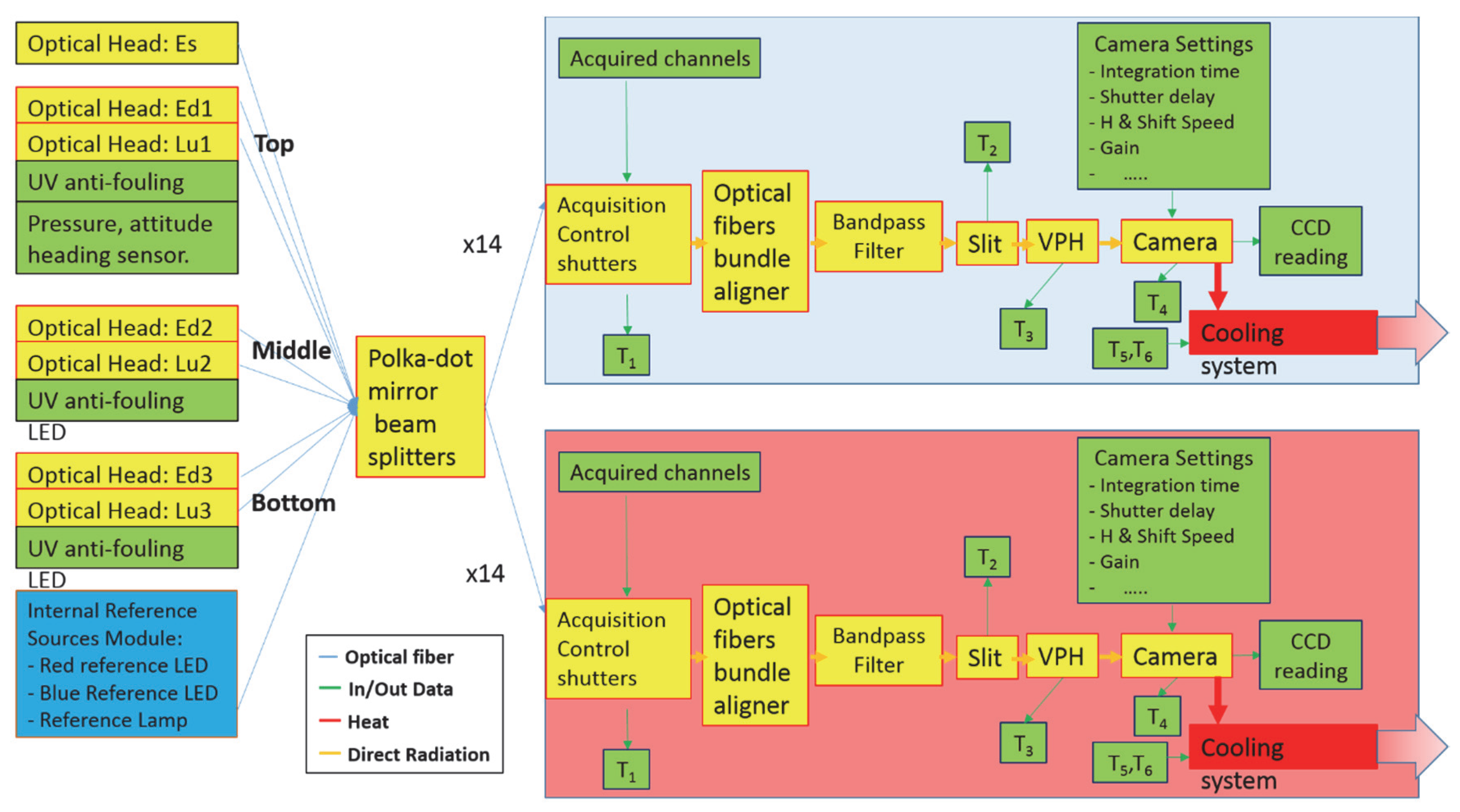
2.1. Optical System Description
- monitor the status of the system: e.g., temperature of different sub-components, power supply, coolant flow, etc.;
- provide ancillary/auxiliary variables for data processing and/or data quality assessment: e.g., sea water temperature and salinity, top arm depth sensor, tilt along two horizontal axes, system heading.
2.2. System Characterization and Calibration
- allow the identification of interactions and dependencies between optical and electronic components;
- identify, evaluate, and correct any systematic disturbances;
- allow the design of the Level-0 to Level-1 data processing, estimate input variables, and verify the radiometric model (see Section 4);
- allow the estimate of the contribution of each component to the uncertainty budget associated with the radiometric measurement (see Section 6).
- full system characterization after complete assembling;
- in-field monitoring;
- post-deployment characterization in case of identified anomaly.
- CCD tracks binning factor;
- full images (saturation checks);
- behavior of dark counts;
- integration time correction factor (shutter delay);
- linearity with optical flux (double aperture; variable radiance source);
- temperature sensitivity (water bath);
- wavelength calibration—atomic line emission sources (pre/post), Fraunhofer lines (field);
- spectral and cross track stray light;
- cosine response (Es);
- polarization sensitivity;
- immersion factors.
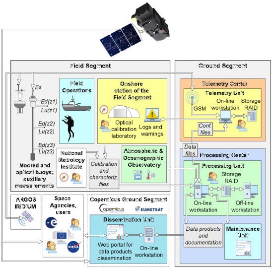
3. EURYBIA Field Segment
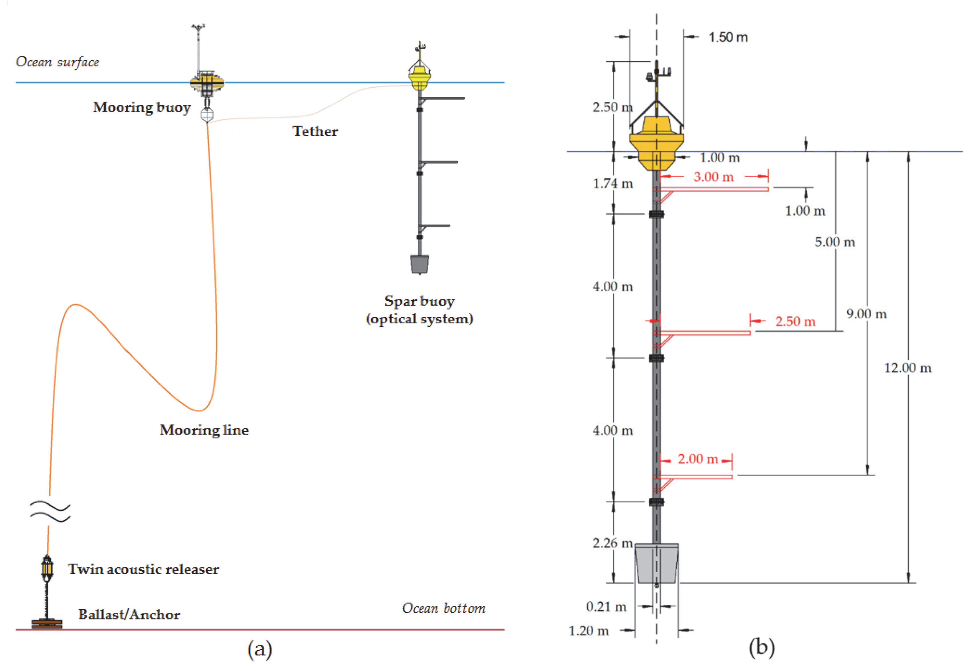
3.1. Optical Buoy
3.2. Mooring Buoy
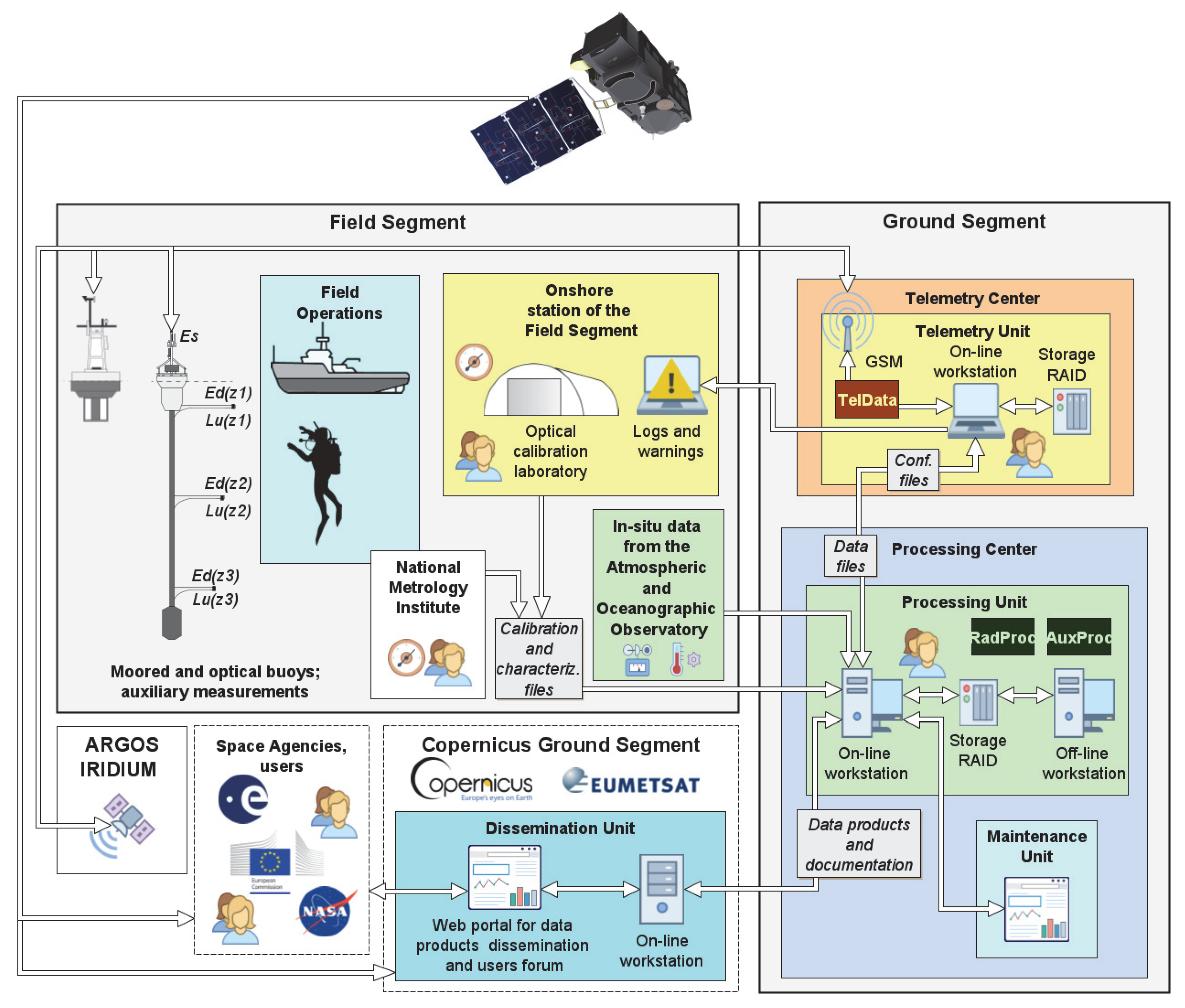
4. Ground Segment
4.1. The Telemetry Center
4.2. The Processing Centre
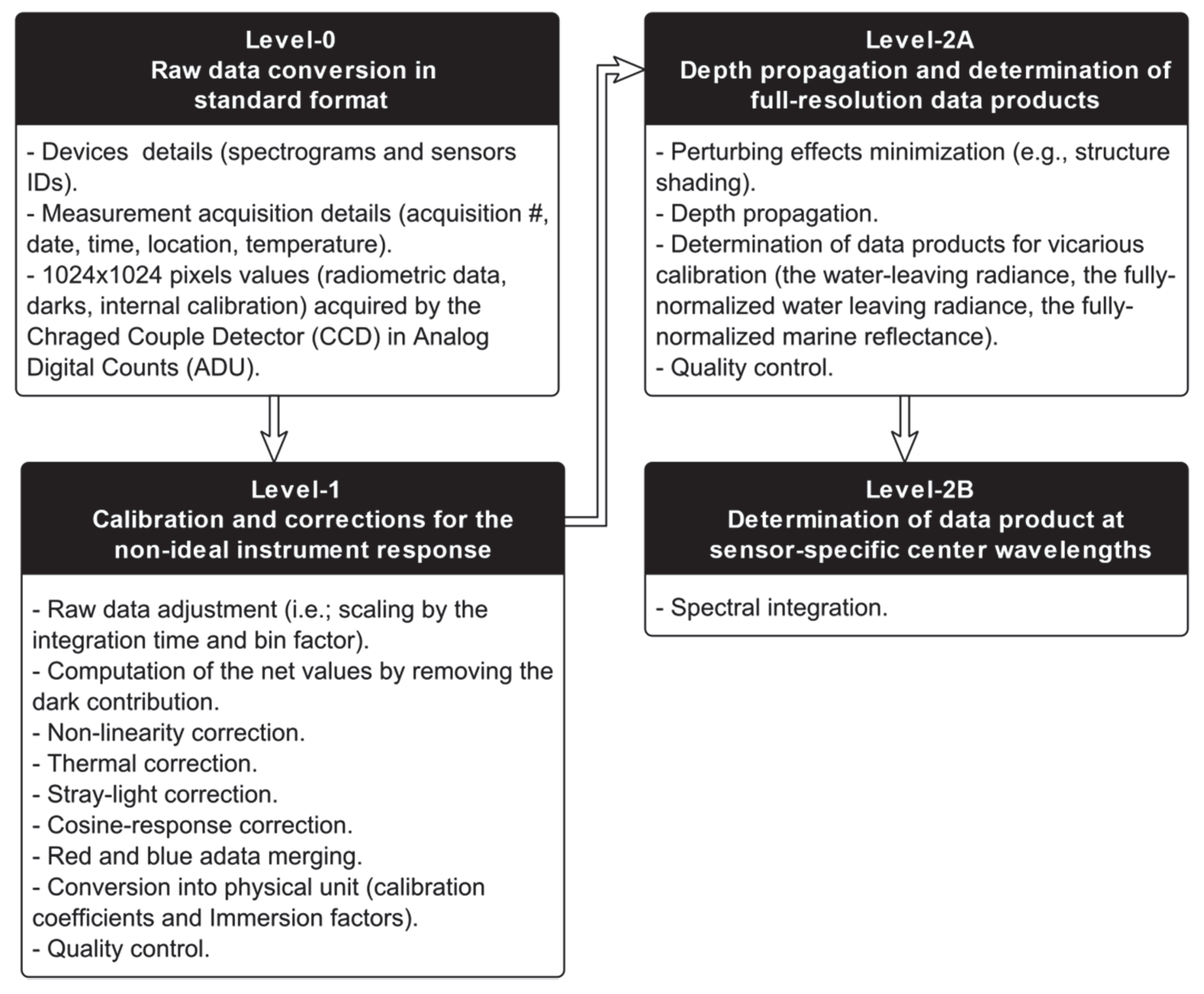
4.2.1. Level-0
4.2.2. Level-1
- represents net radiometric data obtained by subtracting the dark contribution from signal data after scaling the raw CCD readouts by the measurement integration time () and the binning factor (unit of a pixel, pix)— is thus in units of , see for instance [20];
- The term accounts for the non-ideal instrument response due to non-linearity (NL) [21], temperature (T) [22], stray-light (SL) [23,24,25]; non-cosine response (CR) of the above-water irradiance sensor [26,27,28] (with denoting input parameters for the specific correction; e.g., temperatures for T, sun elevation and tilt for CR, etc.);
- indicates the in-air absolute calibration coefficient (i.e., the absolute responsivity) in units of and for the radiance and irradiance data, respectively;
- is the immersion factor accounting for the change in responsivity of the sensor when immersed in water with respect to air (dimensionless).
4.2.3. Level-2A
4.2.4. Level-2B
- Ocean and Land Color Instrument (OLCI); Sentinel 3 missions; Copernicus Program; EU.
- Moderate Resolution Imaging Spectroradiometer (MODIS); Terra/Aqua; NASA; USA.
- Visible Infrared Imaging Radiometer Suite (VIIRS); Suomi NPP, NOAA-20, JPSS-2, JPSS-3; NASA/NOAA; USA.
- Ocean Color Instrument (OCI); Plankton, Aerosol, Cloud, ocean Ecosystem (PACE) program, NASA [39] (https://pace.gsfc.nasa.gov/, planned launch in 2022).
4.3. Quality Assurance and Quality Control
- GOOD indicates the highest quality data for SVC applications (reprocessed data only) or for validation and monitoring (these include near-real-time products release);
- QUESTIONABLE refers to data products derived upon applying significant corrections (e.g., excessive sensor tilting or instability of the instrument response); and
- BAD is applied to data that are unreliable and cannot be used even if the current set of correction schemes are applied (usually caused by unanticipated problems during data acquisition or clouds).
4.4. Data Products Dissemination
- Near Real-Time (NRT) results are delivered once the following operations have been executed: visual data inspection, data correction and calibration, computation of data products such as the normalized water-leaving radiance, and preliminary data quality assurance and control (QA/QC. The timely dissemination of high-quality daily data products derived from in-situ measurements is scoped to release measurements results for the routine assessment and monitoring of orbiting OC remote sensing sensors.
- Post-Deployment Calibration (PDC) results are computed by performing a data re-processing when the optical system has been recovered to shore and re-calibrated. Namely, pre- and post-deployment calibration coefficients are used to account for instruments responsivity change. Any instrument re-characterization for the non-ideal instrument response is also to be taken into consideration.
- Finally, Traceable to Calibration Standards (TCS) of NMI supporting OC-SVC activities are determined by means of an additional data re-processing at the end of the operational cycle of calibration lamps (which is in the order of 50 working hours). At this stage, in fact, the lamps are sent to NMI for traceability. Data products are then recomputed when reference calibration sources are replaced (note that the source stability is continuously monitored at the calibration facilities to allow for prompt actions in the case of out-of-order variations).
4.5. Maintenance Operations
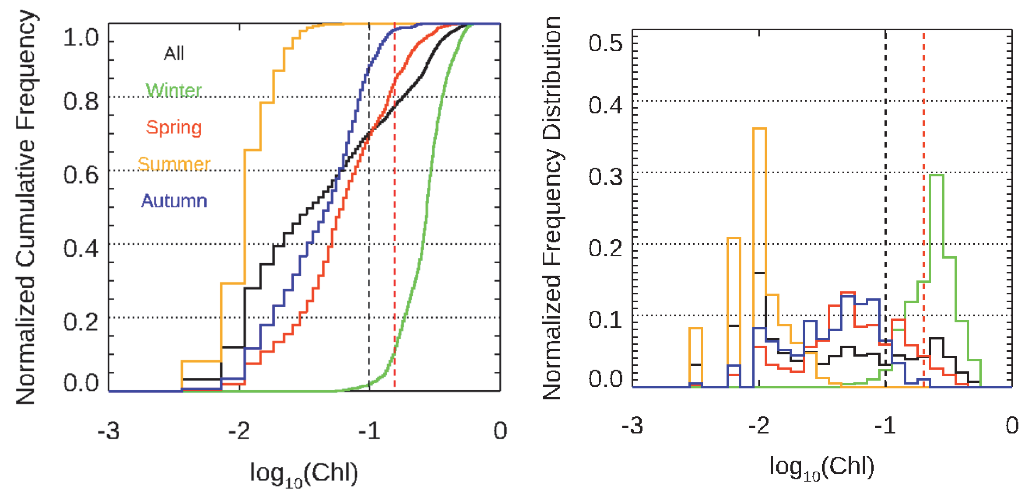
5. Site Characterization
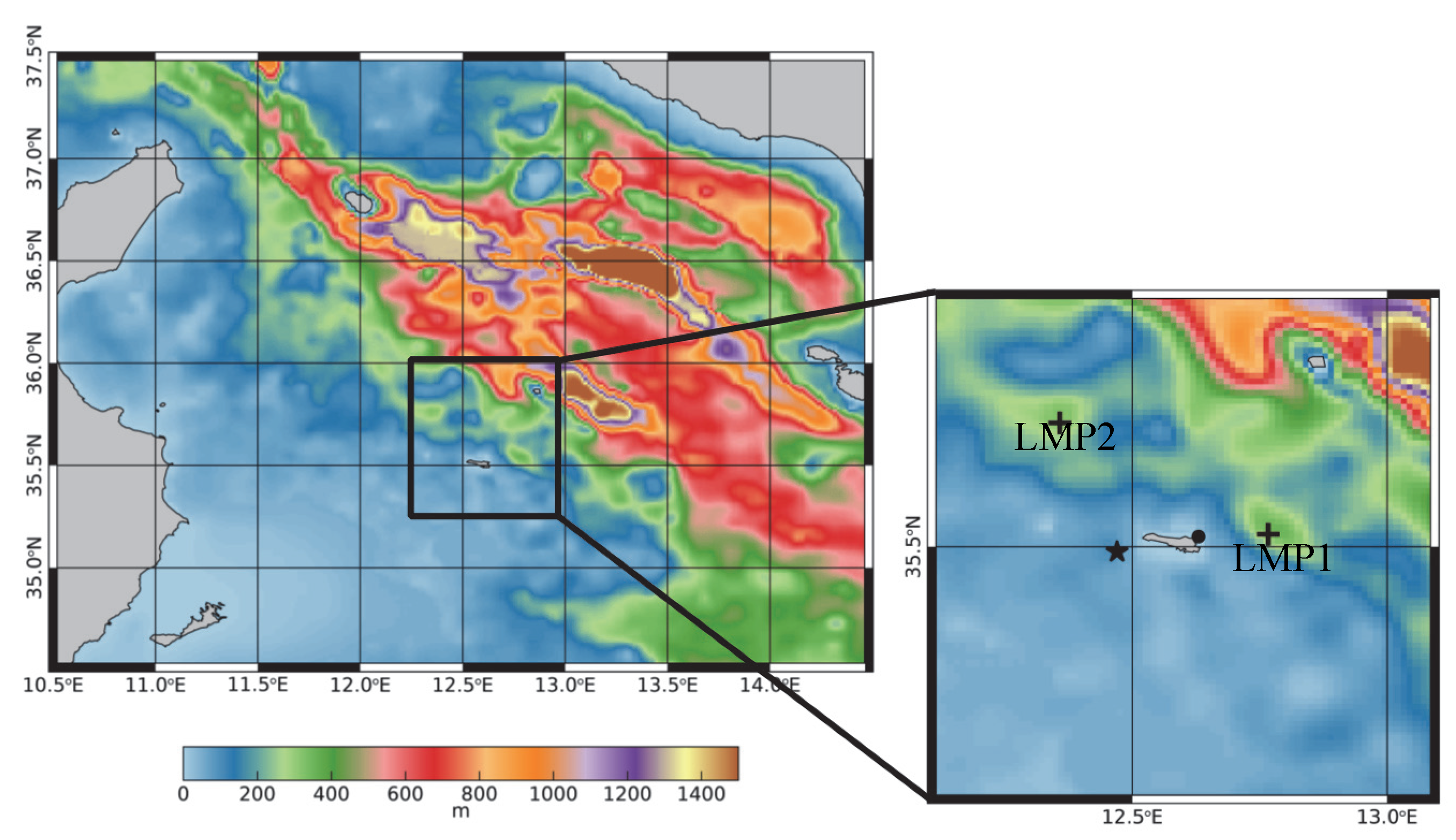
5.1. Location
5.1.1. Geography and Illumination
5.1.2. Existing Infrastructures
5.1.3. Bathymetry
5.2. Oceanographic Properties
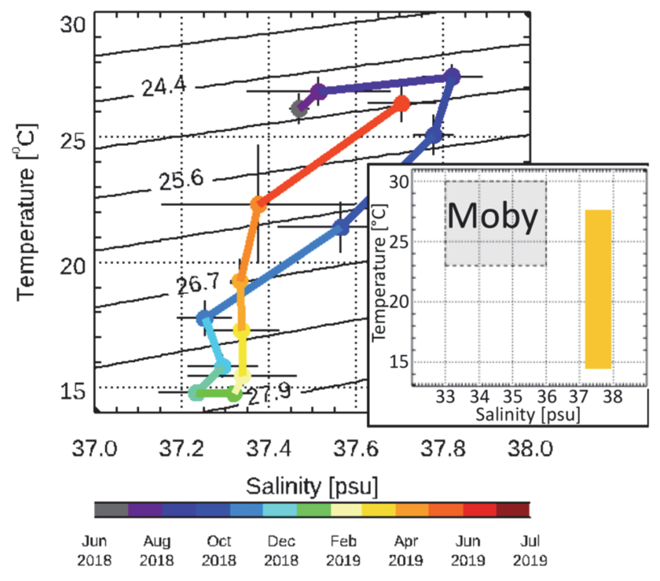
5.2.1. Temperature and Salinity
5.2.2. Currents
5.2.3. Waves
5.2.4. Inherent Optical Properties
5.3. Atmospheric Properties
5.3.1. Meteorology and Local Scale Effects
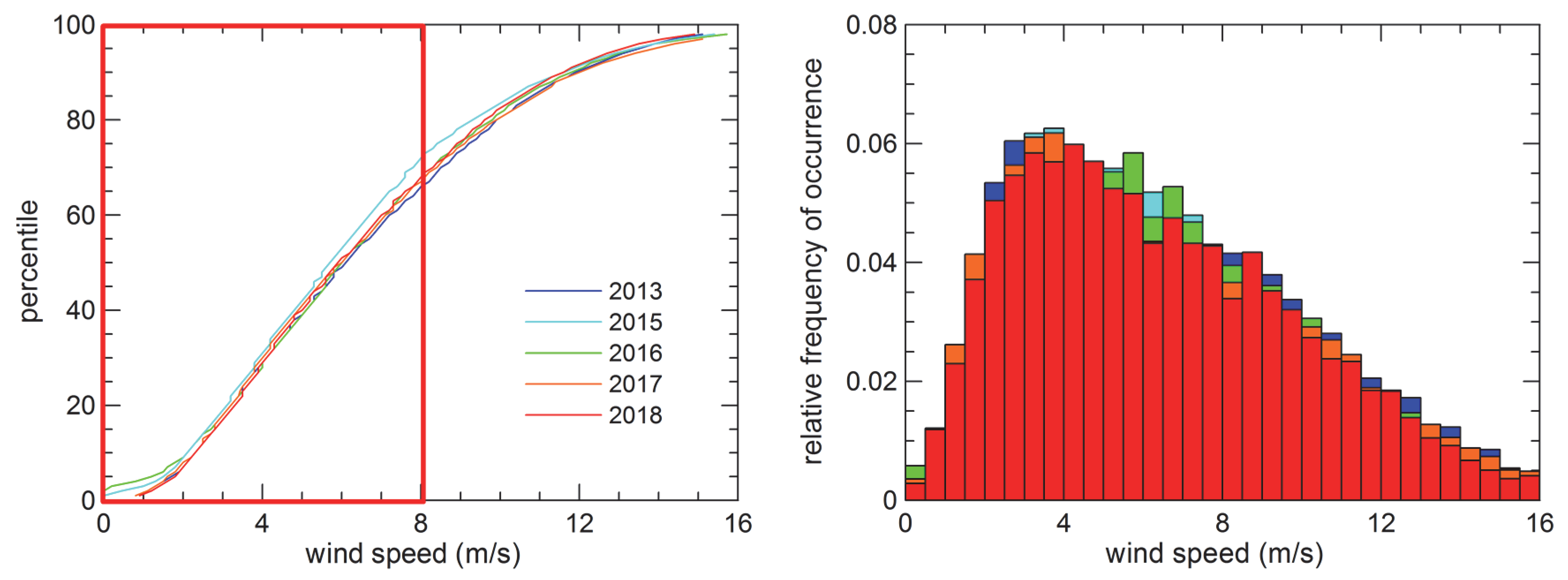
5.3.2. Wind
5.3.3. Cloud Cover
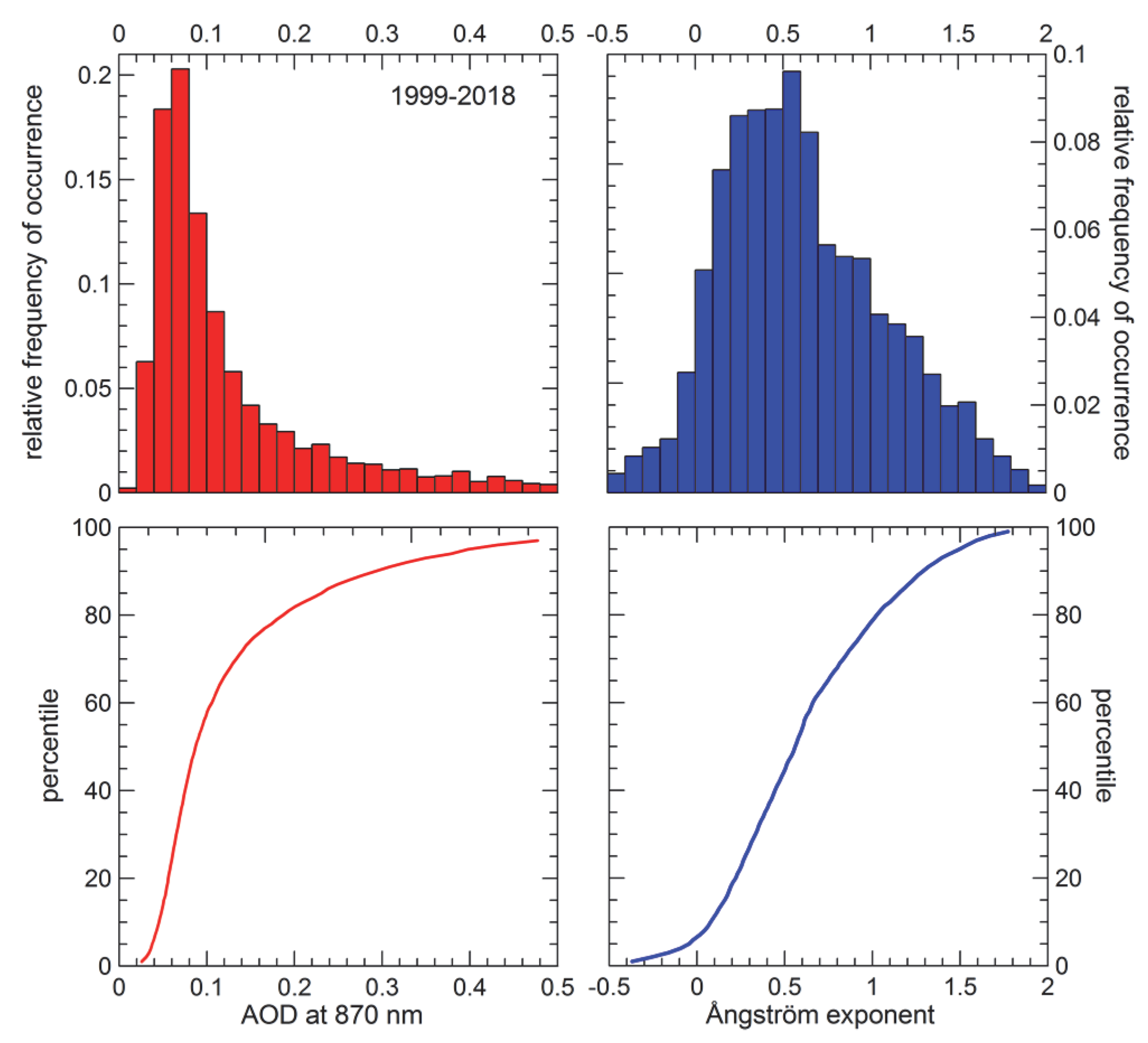
5.3.4. Aerosols
5.3.5. Interfering Gases
5.4. Adjacency Effect
6. Uncertainty Budget
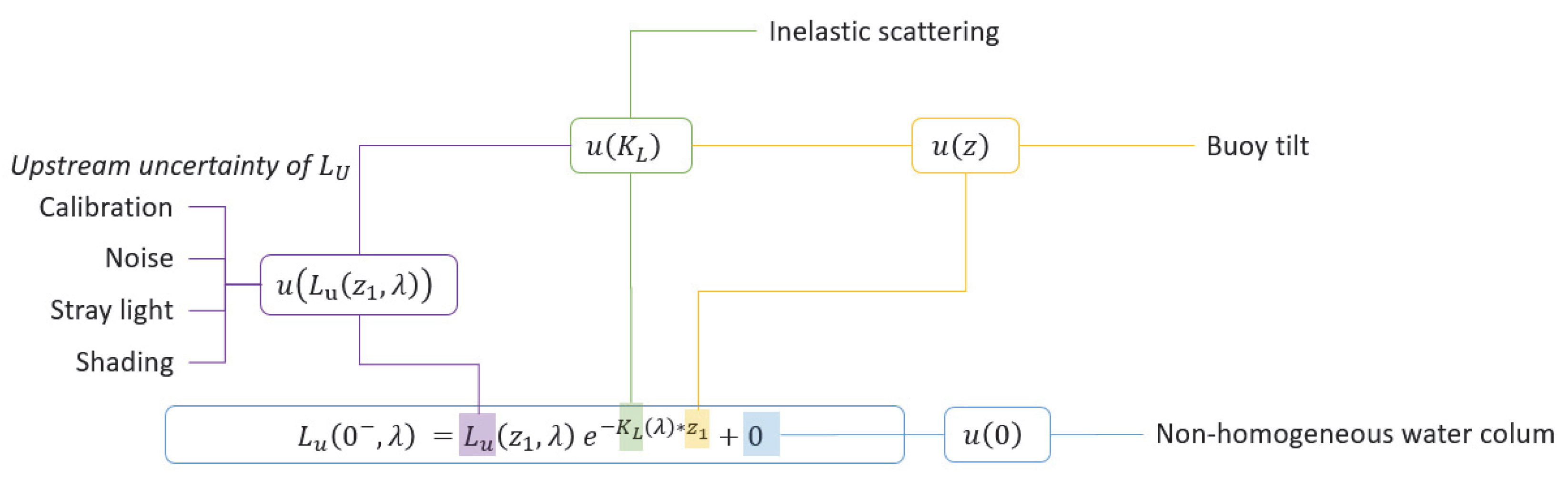
6.1. Uncertainty of the Radiometric Measurement
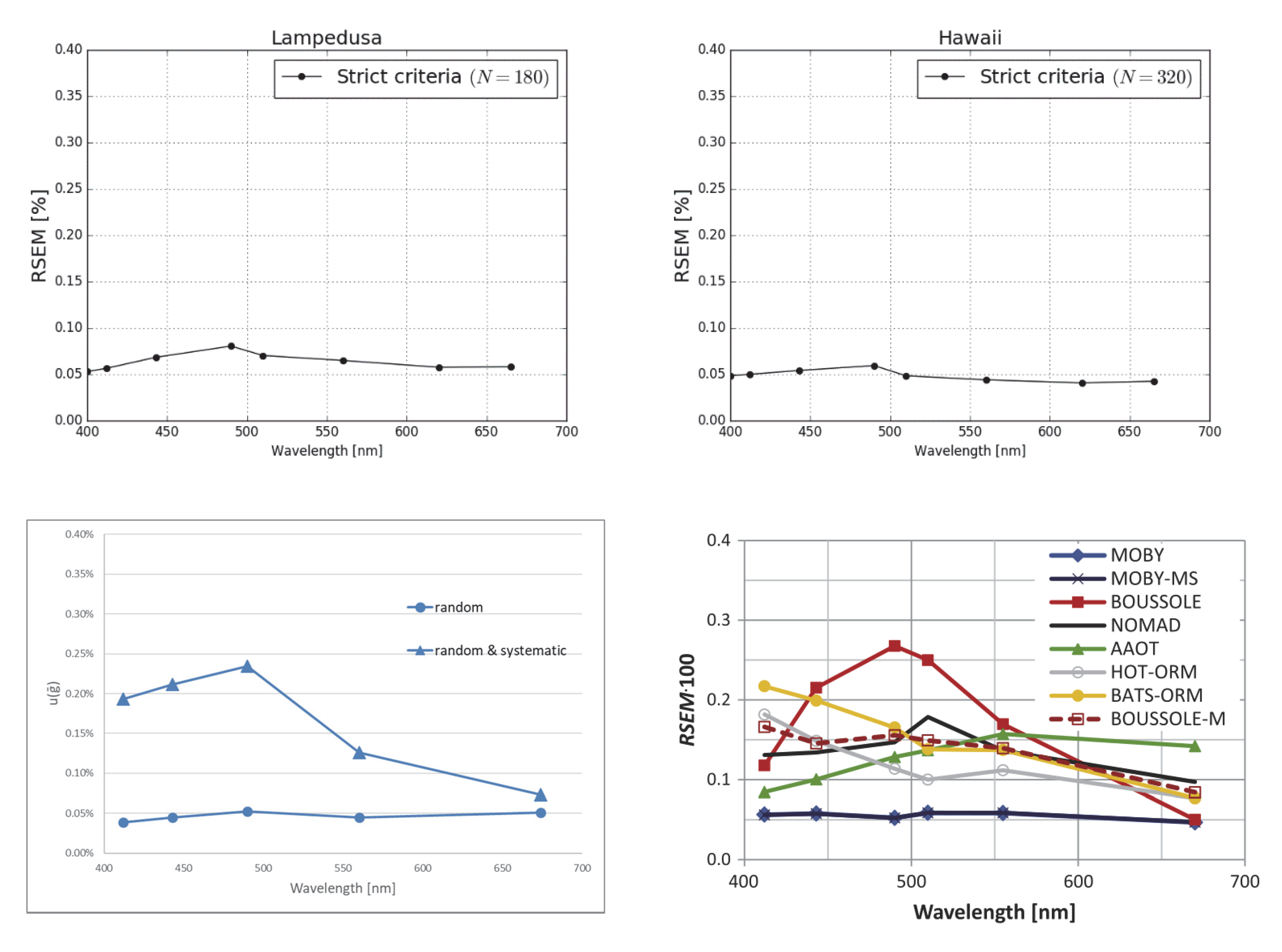
6.2. Uncertainty of the SVC Gains
- 5 × 5 box centered on single pixels;
- For each pixel, sensor zenith angle should be below 56° and the sun zenith angle below 70°;
- Excluding pixels contaminated by known disturbances, i.e. masked with at least one of the following flags: CLOUD, CLOUD_AMBIGUOUS, CLOUD_MARGIN, INVALID, COSMETIC, SATURATED, SUSPECT, HISOLZEN, HIGHGLINT, SNOW_ICE, WHITECAPS, ANNOT_ABSO_D, ANNOT_MIXR1, ANNOT_TAU06, RWNEG_O2, RWNEG_O3, RWNEG_O4, RWNEG_O5, RWNEG_O6, RWNEG_O7, RWNEG_O8;
- All pixels within the 5 × 5 region of interest (ROI) should be valid;
- Mean chlorophyll within the ROI should be below 0.2 mg/m3;
- Mean aerosol optical depth (AOD) for the channel at 865 nm should be below 0.15;
- Coefficient of Variation should be below 0.15 for remote sensing reflectances at bands between 412 and 560 nm, where µ* and σ* are mean and standard deviation, respectively, computed after the removal of pixel outliers. A pixel is considered as an outlier for variable xi if |xi - µ| < 1.5 σ where µ is the mean and σ is the standard deviation of that variable over the 5x5 box.
- Consider, for each potential match-up, a ROI of 5 × 5 OLCI pixels (full resolution), consistent with EUMETSAT protocols for SVC as defined previously;
- Consider all OLCI metadata and ancillary data at pixel level (wind speed, pressure, geometry);
- Consider OLCI aerosol optical thickness and Angstrom coefficient;
- Identify, for each pixel, the best matching aerosol model in the OLCI LUTs;
- Given geometry and ancillary data, compute and by the OLCI LUTs (Rayleigh + aerosol), as done in OLCI atmospheric correction;
- Compute and by their local standard-deviation over the ROI.
- A purely random case: the uncertainty sources are all assigned to the random component.
- A mix between random and systematic sources (Figure 14, bottom-left, triangles): in Table 4, Table 5, Table 6, Table 7 and Table 8, an attempt is made to assign the uncertainty of various sources to the systematic component, only (i.e., without any random counterpart). Note that the global uncertainty of a given source is identical to the previous case (i.e., the quadratic sum of the random and systematic components equals the square random component of the previous case).
7. Discussion and Conclusions
Author Contributions
Funding
Acknowledgments
Conflicts of Interest
Abbreviations
| ACTRIS | Aerosol, Clouds and Trace Gases |
| ADCP | Acoustic Current Doppler profiler |
| ADU | Analog Digital Counts |
| AE | Adjacency Effect |
| AERONET | Aerosol Robotic Network |
| AOD | Aerosol Optical Depth |
| AOT | Aerosol Optical Thickness |
| BOUSSOLE | BOUée pour l’acquiSition d’une Série Optique à Long termE |
| BRDF | Bidirectional Reflectance Distribution Function |
| BSG | Blue Spectro Graph |
| C3S | Copernicus Climate Change Service |
| CCD | Charged Coupled Device |
| CDOM | Coloured Dissolved Organic Matter |
| CF | Cloud Fraction |
| CMEMS | Copernicus Marine Environment Monitoring Service |
| CTD | Conductivity Temperature Depth |
| CTP | Cloud Top Pressure |
| CV | Coefficient of Variation |
| ESA | European Space Agency |
| EUB | Estimated Uncertainty Budget |
| EUMETSAT | European Organisation for the Exploitation of Meteorological Satellites |
| EURYBIA | EUropean RadiometrY Buoy and InfrAstructure |
| FOV | Field of View |
| FRM | Fiducial Reference Measurements |
| FWHM | Full Width at Half Maximum |
| GS | Ground Segment |
| GUM | Guide to the expression of Uncertainty in Measurement |
| ICOS | Integrated Carbon Observation System |
| IOCCG | International Ocean Colour Coordinating Group |
| IOPs | Inherent Optical Properties |
| LUT | Look-up Tables |
| MarONet | Marine Optical Network |
| MC | Monte Carlo |
| MFRSR | Multi Filter Rotating Shadowband Radiometer |
| MOBY | Marine Optical BuoY |
| MODIS | Moderate Resolution Imaging Spectroradiometer |
| NASA | National Aeronautics and Space Administration |
| NIR | Near-Infrared |
| NMI | National Metrology Institute |
| NOAA | National Oceanic and Atmospheric Administration |
| NRT | Near Real-Time |
| OC-SVC | Ocean Colour System Vicarious Calibration |
| OLCI | Ocean and Land Colour Instrument |
| OMI | Ozone Monitoring Instrument |
| PACE | Plankton, Aerosol, Cloud, ocean Ecosystem |
| PDC | Post-Deployment Calibration |
| PM10 | Particulate Matter smaller than 10µm |
| QC/QA | Quality Control / Quality Assurance |
| ROI | Region of Interest |
| RSEM | Relative Standard Error of the Mean |
| RSG | Red Spectro Graph |
| S3 | Sentinel-3 |
| SDY | Sequential Day of the Year |
| SI | International System of Units |
| SeaWiFS | Sea-viewing Wide Field-of-view Sensor |
| SRF | Spectral Response Function |
| SST | Sea Surface Temperature |
| TCS | Traceable to Calibration Standards |
| TOA | Top Of Atmosphere |
| TOC | Total Ozone Column |
| UTC | Coordinated Universal Time |
| VIIRS | Visible Infrared Imaging Radiometer Suite |
| VPH | Volume Phase Holographic |
References
- Ansper, A.; Alikas, K. Retrieval of Chlorophyll a from Sentinel-2 MSI data for the European Union water framework directive reporting purposes. Remote Sens. 2018, 11, 64. [Google Scholar] [CrossRef] [Green Version]
- Groom, S.; Sathyendranath, S.; Ban, Y.; Bernard, S.; Brewin, R.; Brotas, V.; Brockmann, C.; Chauhan, P.; Choi, J.; Chuprin, A.; et al. Satellite ocean colour: Current status and future perspective. Front. Mar. Sci. 2019, 6, 485. [Google Scholar] [CrossRef] [Green Version]
- Mazeran, C.; Brockmann, C.; Ruddick, K.; Voss, K.J.; Zagolsky, F.; Antoine, D.; Bialek, A.; Brando, V.; Donlon, C.; Franz, B.A.; et al. Requirements for Copernicus Ocean Colour Vicarious Calibration Infrastructure; EUMETSAT Study. 2017. Available online: https://www.eumetsat.int/website/wcm/idc/idcplg?IdcService=GET_FILE&dDocName=PDF_COP_OCEAN_COL_CAL&RevisionSelectionMethod=LatestReleased&Rendition=Web (accessed on 28 February 2020).
- Zibordi, G.; Mélin, F.; Voss, K.J.; Johnson, B.C.; Franz, B.A.; Kwiatkowska, E.; Huot, J.-P.; Wang, M.; Antoine, D. System vicarious calibration for ocean color climate change applications: Requirements for in-situ data. Remote Sens. Environ. 2015, 361–369. [Google Scholar] [CrossRef]
- Lerebourg, C.; Vendt, R.; Donlon, C. Fiducial reference measurements for satellite ocean colour (FRM4SOC). In Proceedings of the D-240 Proceedings of WKP-1 (PROC-1) Report of the International Workshop; European Space Agency: ESRIN: Frascati, Italy, 2016. [Google Scholar]
- Gordon, H.R. In-orbit calibration strategy for ocean color sensors. Remote Sens. Environ. 1998, 63, 265–278. [Google Scholar] [CrossRef]
- IOCCG. International Network for Sensor Inter-Comparison and Uncertainty Assessment for Ocean Color Radiometry (IN-SITU-OCR); International Ocean Color Coordinating Group: Dartmouth, NS, Canada, 2012. [Google Scholar]
- Donlon, C. Sentinel-3 Mission Requirements Traceability Document (MRTD); European Space Agency: Noordwijk, The Netherlands, 2011. [Google Scholar]
- Clark, D.K.; Yarbrough, M.; Feinholz, M.; Flora, S.; Broenkow, W.; Johnson, C.B.; Brown, S.W.; Yuen, M.; Mueller, J. MOBY, a radiometric buoy for performance monitoring and vicarious calibration of satellite ocean color sensors: Measurement and data analysis protocols. In Ocean Optics Protocols for Satellite Ocean Color Sensor Validation, Revision 3, Volume 2; Mueller, J.L., Fargion, G.S., Eds.; NASA Goddard Space Flight Center: Greenbelt, MD, USA, 2002; Volume NASA/TM--2002-21004, pp. 138–170. [Google Scholar]
- Antoine, D.; Guevel, P.; Desté, J.-F.; Bécu, G.; Louis, F.; Scott, A.J.; Bardey, P. The “boussole” buoy—A new transparent-to-swell taut mooring dedicated to marine optics: Design, tests, and performance at sea. J. Atmos. Ocean. Technol. 2008, 25, 968–989. [Google Scholar] [CrossRef]
- Zibordi, G.; Mélin, F. An evaluation of marine regions relevant for ocean color system vicarious calibration. Remote Sens. Environ. 2017, 190, 122–136. [Google Scholar] [CrossRef]
- Zibordi, G.; Mélin, F.; Talone, M.; European Commission; Joint Research Centre. System Vicarious Calibration for Copernicus Ocean Colour Missions: Updated Requirements and Recommendations for a European Site; Publications Office of the European Union: Brussels, Belgium, 2017; ISBN 978-92-79-75340-4. [Google Scholar]
- Bulgarelli, B.; Zibordi, G. Adjacency radiance around a small island: Implications for system vicarious calibrations. Appl. Opt. 2020, 59, C63–C69. [Google Scholar] [CrossRef]
- EUMETSAT. Sentinel-3 OLCI Marine User Handbook, Version 1H, Ref. EUM/OPS-SEN3/MAN/17/907205; Technical Report; EUMETSAT: Darmstadt, Germany, 2018. [Google Scholar]
- Voss, K.J.; Yarbrough, M.A.; Johnson, B.C.; Feinholz, M.E.; Gleason, A.; Flora, S.J. Present Status of the Marine Optical Buoy (MOBY) Refresh and MOBY-Net; MOBY: Dubrovnik, Croatia, 2018. [Google Scholar]
- Feinholz, M.; Johnson, C.B.; Voss, K.; Yarbrough, M.; Flora, S. Immersion coefficient for the Marine Optical Buoy (MOBY) radiance collectors. J. Res. Natl. Inst. Stand. Technol. 2017, 122, 1–9. [Google Scholar] [CrossRef]
- Voss, K.J.; Johnson, C.B.; Yarbrough, M.A.; Gleason, A.; Flora, S.J.; Feinholz, M.E.; Peters, D.; Houlihan, T.; Mundell, S.; Yarbrough, S. An overview of the Marine Optical Buoy (MOBY): Past, present and future. In Proceedings of the D-240 FRM4SOC-PROC1 Proceedings of WKP-1 (PROC-1) Fiducial Reference Measurements for Satellite Ocean Colour (FRM4SOC), Tartu, Estonia, 8–13 May 2017. [Google Scholar]
- Johnson, B.C.; Voss, K.J.; Yarbrough, M.A.; Flora, S.J.; Feinholz, M.E.; Peters, D.; Houlihan, T.; Mundell, S. MOBY radiometric calibration and associated uncertainties. In Proceedings of the D-240 FRM4SOC-PROC1 Proceedings of WKP-1 (PROC-1) Fiducial Reference Measurements for Satellite Ocean Colour (FRM4SOC), Tartu, Estonia, 8–13 May 2017. [Google Scholar]
- Barden, S.C.; Arns, J.A.; Colburn, W.S. Volume-Phase Holographic Gratings and Their Potential for Astronomical Applications; D’Odorico, S., Ed.; SPIE: Kona, HI, USA, 1998; pp. 866–876. [Google Scholar] [CrossRef] [Green Version]
- Flora, S.J.; Broenkow, W.W. Data Reduction Algorithms for the Marine Optical Buoy and Marine Optical System; Moss Landing Marine Laboratories Technical Publication 08-X Moss Landing, CA 95039. 2008, p. 16. Available online: http://data.moby.mlml.calstate.edu/timeseries/other_reports/data%20reduction%20algorithms%20for%20the%20marine%20optical%20buoy.pdf (accessed on 28 February 2020).
- Vabson, V.; Kuusk, J.; Ansko, I.; Vendt, R.; Alikas, K.; Ruddick, K.; Ansper, A.; Bresciani, M.; Burmester, H.; Costa, M.; et al. Laboratory intercomparison of radiometers used for satellite validation in the 400–900 nm range. Remote Sens. 2019, 11, 1101. [Google Scholar] [CrossRef] [Green Version]
- Zibordi, G.; Talone, M.; Jankowski, L. Response to temperature of a class of in-situ hyperspectral radiometers. J. Atmos. Ocean. Technol. 2017, 34, 1795–1805. [Google Scholar] [CrossRef]
- Torrecilla, E.; Pons, S.; Vilaseca, M.; Piera, J.; Pujol, J. Stray-light correction of in-water array spectroradiometers. Effects on underwater optical measurements. In Proceedings of the OCEANS 2008, Quebec City, QC, Canada, 15–18 September 2008; pp. 1–5. [Google Scholar] [CrossRef]
- Feinholz, M.E.; Flora, S.J.; Yarbrough, M.A.; Lykke, K.R.; Brown, S.W.; Johnson, B.C.; Clark, D.K. Stray light correction of the marine optical system. J. Atmos. Ocean. Technol. 2009, 26, 57–73. [Google Scholar] [CrossRef]
- Talone, M.; Zibordi, G.; Ansko, I.; Banks, A.C.; Kuusk, J. Stray light effects in above-water remote-sensing reflectance from hyperspectral radiometers. Appl. Opt. 2016, 55, 3966. [Google Scholar] [CrossRef] [PubMed]
- Seckmeyer, G.; Bernhard, G. Cosine Error Correction of Spectral UV-Irradiances; Stamnes, K.H., Ed.; SPIE: Tromso, Norway, 1993; pp. 140–151. [Google Scholar] [CrossRef]
- Zibordi, G.; Bulgarelli, B. Effects of cosine error in irradiance measurements from field ocean color radiometers. Appl Opt. 2007, 46, 5529–5538. [Google Scholar] [CrossRef] [PubMed]
- Zibordi, G.; Voss, K.J.; Johnson, C.B.; Mueller, J.L. Protocols for satellite ocean colour data validation. In-Situ Opt. Radiom. 2019, 3. [Google Scholar] [CrossRef]
- D’Alimonte, D.; Zibordi, G.; Kajiyama, T. Effects of integration time on in-water radiometric profiles. Opt. Express 2018, 26, 5908. [Google Scholar] [CrossRef] [PubMed]
- Kajiyama, T.; D’Alimonte, D.; Cunha, J.C. A high-performance computing framework for Monte Carlo ocean color simulations. Concurr. Comput. Pract. Exp. 2017, 29, e3860. [Google Scholar] [CrossRef] [Green Version]
- D’Alimonte, D.; Kajiyama, T. Effects of light polarization and waves slope statistics on the reflectance factor of the sea surface. Opt. Express 2016, 24, 7922. [Google Scholar] [CrossRef] [Green Version]
- Mueller, J.L. Reduced Uncertainties in Measurements of Water-Leaving Radiance, and Other Optical Properties, Using Radiative Transfer Models and Empirical Data Analysis; CHORS, San Diego State University Research Foundation: San Diego, CA, USA, 2007. [Google Scholar]
- Voss, K.J.; Gordon, H.R.; Flora, S.; Johnson, B.C.; Yarbrough, M.; Feinholz, M.; Houlihan, T. A method to extrapolate the diffuse upwelling radiance attenuation coefficient to the surface as applied to the Marine Optical Buoy (MOBY). J. Atmos. Ocean. Technol. 2017, 34, 1423–1432. [Google Scholar] [CrossRef]
- Austin, R.W. The remote sensing of spectral radiance from below the ocean surface. In Optical Aspects of Oceanography; Jerlov, N.G., Steemann-Nielsen, E., Eds.; Academic Press Inc.: London, UK, 1974; pp. 317–344. [Google Scholar]
- Gordon, H.R.; Morel, A.Y. Remote Assessment of Ocean Color for Interpretation of Satellite Visible Imagery: A Review; Springer: New York, NY, USA, 2010; ISBN 978-1-118-66370-7. [Google Scholar]
- Voss, K.J.; Flora, S. Spectral dependence of the seawater–air radiance transmission coefficient. J. Atmos. Ocean. Technol. 2017. [Google Scholar] [CrossRef]
- Gordon, H.R.; Wang, M. Influence of oceanic whitecaps on atmospheric correction of ocean-color sensors. Appl. Opt. 1994, 33, 7754. [Google Scholar] [CrossRef]
- Morel, A.; Antoine, D.; Gentili, B. Bidirectional reflectance of oceanic waters: Accounting for raman emission and varying particle scattering phase function. Appl. Opt. 2002, 41, 6289. [Google Scholar] [CrossRef] [PubMed]
- Werdell, P.J.; Behrenfeld, M.J.; Bontempi, P.S.; Boss, E.; Cairns, B.; Davis, G.T.; Franz, B.A.; Gliese, U.B.; Gorman, E.T.; Hasekamp, O.; et al. The plankton, aerosol, cloud, ocean ecosystem mission: Status, science, advances. Bull. Am. Meteorol. Soc. 2019, 100, 1775–1794. [Google Scholar] [CrossRef]
- Grasso, M.; Pedley, H.M. The pelagian islands: A new geological interpretation from sedimentological and tectonic studies and its bearing on the evolution of the central Mediterranean Sea (Pelagian Block). Geol. Romana 1985, 24, 13–34. [Google Scholar]
- Ciardini, V.; Contessa, G.M.; Falsaperla, R.; Gómez-Amo, J.L.; Meloni, D.; Monteleone, F.; Pace, G.; Piacentino, S.; Sferlazzo, D.; Sarra, A. di Global and Mediterranean climate change: A short summary. Annali Dell’Istituto Superiore Di Sanità 2016. [Google Scholar] [CrossRef]
- di Sarra, A.; Bommarito, C.; Anello, F.; Di Iorio, T.; Meloni, D.; Monteleone, F.; Pace, G.; Piacentino, S.; Sferlazzo, D. Assessing the quality of shortwave and longwave irradiance observations over the ocean: One year of high-time-resolution measurements at the lampedusa oceanographic observatory. J. Atmos. Ocean. Technol. 2019, 36, 2383–2400. [Google Scholar] [CrossRef]
- Casasanta, G.; di Sarra, A.; Meloni, D.; Monteleone, F.; Pace, G.; Piacentino, S.; Sferlazzo, D. Large aerosol effects on ozone photolysis in the Mediterranean. Atmos. Environ. 2011, 45, 3937–3943. [Google Scholar] [CrossRef]
- di Sarra, A.; Fua, D.; Cacciani, M.; Di Iorio, T.; Disterhoft, P.; Meloni, D.; Monteleone, F.; Piacentino, S.; Sferlazzo, D. Determination of ultraviolet cosine-corrected irradiances and aerosol optical thickness by combined measurements with a Brewer spectrophotometer and a multifilter rotating shadowband radiometer. Appl. Opt. 2008, 47, 6142. [Google Scholar] [CrossRef]
- Meloni, D.; Di Biagio, C.; di Sarra, A.; Monteleone, F.; Pace, G.; Sferlazzo, D.M. Accounting for the solar radiation influence on downward longwave irradiance measurements by pyrgeometers. J. Atmos. Ocean. Technol. 2012, 29, 1629–1643. [Google Scholar] [CrossRef]
- Harrison, A.W.; Coombes, C.A. Performance validation of the Gueymard sky radiance model. Atmos Ocean 1989, 27, 565–576. [Google Scholar] [CrossRef]
- Coombes, C.A.; Harrison, A.W. Calibration of a three-component angular distribution model of sky radiance. Atmos Ocean 1988, 26, 183–192. [Google Scholar] [CrossRef]
- Gregg, W.W.; Carder, K.L. A simple spectral solar irradiance model for cloudless maritime atmospheres. Linmol. Ocean. 1990, 35, 1657–1675. [Google Scholar] [CrossRef]
- Volpe, G.; Dionisi, D.; Brando, V.; Colella, S.; Bracaglia, M.; Pitarch, J.; Falcini, F.; Sammartino, M.; Benincasa, M.; Santoleri, R. IOPs Continuous Measurements for Ocean Monitoring and Calibration and Validation of Satellite Data; EGU: Vienna, Austria, 2018; Volume 20, p. 16329. [Google Scholar]
- Petzold, T.J. Volume Scattering Functions for Selected Ocean Waters; Scripps Institution of Oceanography: San Diego, CA, USA, 1972. [Google Scholar]
- Maritorena, S.; Morel, A.; Gentili, B. Diffuse reflectance of oceanic shallow waters: Influence of water depth and bottom albedo. Limnol. Ocean. 1994, 39, 689–703. [Google Scholar] [CrossRef]
- Simoncelli, S.; Fratianni, C.; Pinardi, N.; Grandi, A.; Drudi, M.; Oddo, P.; Dobricic, S.; Mediterranean Sea Physical Reanalysis (CMEMS MED-Physics) [Data Set]. Copernicus Monitoring Environment Marine Service (CMEMS). 2019. Available online: https://doi.org/10.25423/MEDSEA_REANALYSIS_PHYS_006_004 (accessed on 28 February 2020).
- Jouini, M.; Béranger, K.; Arsouze, T.; Beuvier, J.; Thiria, S.; Crépon, M.; Taupier-Letage, I. The sicily channel surface circulation revisited using a neural clustering analysis of a high-resolution simulation: The sicily channel surface circulation. J. Geophys. Res. Ocean. 2016, 121, 4545–4567. [Google Scholar] [CrossRef] [Green Version]
- Copernicus Climate Change Service (C3S). ERA5: Fifth Generation of ECMWF Atmospheric Reanalyses of the Global Climate. Copernicus Climate Change Service Climate Data Store (CDS), June 2019. 2017. Available online: https://cds.climate.copernicus.eu/cdsapp#!/home (accessed on 28 February 2020).
- Pace, G.; Cremona, G.; di Sarra, A.; Meloni, D.; Monteleone, F.; Sferlazzo, D.; Zaninin, G. Continuous vertical profiles of temperature and humidity at Lampedusa island. In Proceedings of the 9th International Symposium on Tropospheric Profiling, L’Aquila, Italy, 3–7 September 2012. [Google Scholar]
- Kotsias, G.; Lolis, C.J. A study on the total cloud cover variability over the Mediterranean region during the period 1979–2014 with the use of the ERA-Interim database. Theor. Appl. Climatol. 2018, 134, 325–336. [Google Scholar] [CrossRef]
- Meloni, D.; di Sarra, A.; Biavati, G.; DeLuisi, J.J.; Monteleone, F.; Pace, G.; Piacentino, S.; Sferlazzo, D.M. Seasonal behavior of Saharan dust events at the Mediterranean island of Lampedusa in the period 1999–2005. Atmos. Environ. 2007, 41, 3041–3056. [Google Scholar] [CrossRef]
- Long, C.N.; Ackerman, T.P. Identification of clear skies from broadband pyranometer measurements and calculation of downwelling shortwave cloud effects. J. Geophys. Res. Atmos. 2000, 105, 15609–15626. [Google Scholar] [CrossRef]
- Trisolino, P.; di Sarra, A.; Anello, F.; Bommarito, C.; Di Iorio, T.; Meloni, D.; Monteleone, F.; Pace, G.; Piacentino, S.; Sferlazzo, D. A long-term time series of global and diffuse photosynthetically active radiation in the Mediterranean: Interannual variability and cloud effects. Atmos. Chem. Phys. 2018, 18, 7985–8000. [Google Scholar] [CrossRef] [Green Version]
- Min, Q.; Wang, T.; Long, C.N.; Duan, M. Estimating fractional sky cover from spectral measurements. J. Geophys. Res. 2008, 113, D20208. [Google Scholar] [CrossRef] [Green Version]
- Pace, G.; di Sarra, A.; Meloni, D.; Piacentino, S.; Chamard, P. Aerosol optical properties at Lampedusa (Central Mediterranean). 1. Influence of transport and identification of different aerosol types. Atmos. Chem. Phys. 2006, 6, 697–713. [Google Scholar] [CrossRef] [Green Version]
- Meloni, D.; di Sarra, A.; Pace, G.; Monteleone, F. Aerosol optical properties at Lampedusa (Central Mediterranean). 2. Determination of single scattering albedo at two wavelengths for different aerosol types. Atmos. Chem. Phys. 2006, 6, 715–727. [Google Scholar] [CrossRef] [Green Version]
- di Sarra, A.; Sferlazzo, D.; Meloni, D.; Anello, F.; Bommarito, C.; Corradini, S.; De Silvestri, L.; Di Iorio, T.; Monteleone, F.; Pace, G.; et al. Empirical correction of multifilter rotating shadowband radiometer (MFRSR) aerosol optical depths for the aerosol forward scattering and development of a long-term integrated MFRSR-Cimel dataset at Lampedusa. Appl. Opt. 2015, 54, 2725. [Google Scholar] [CrossRef] [PubMed]
- Calzolai, G.; Nava, S.; Lucarelli, F.; Chiari, M.; Giannoni, M.; Becagli, S.; Traversi, R.; Marconi, M.; Frosini, D.; Severi, M.; et al. Characterization of PM 10 sources in the central Mediterranean. Atmos. Chem. Phys. 2015, 15, 13939–13955. [Google Scholar] [CrossRef] [Green Version]
- Bulgarelli, B.; Zibordi, G. Analysis of Adjacency Effects for Copernicus Ocean Colour Missions. 2018. Available online: https://www.semanticscholar.org/paper/Analysis-of-adjacency-effects-for-Copernicus-Ocean-Barbara-Giuseppe/018cffaf395d3cf29f2254073bbc7b5f7b8c4c8e (accessed on 2 April 2020).
- BIPM; IEC; IFCC; ILAC; ISO; IUPAC; IUPAP; OMIL. Evaluation of Measurement Data—Guide to the Expression of Uncertainty in Measurement; GUM 1995 with minor corrections; JCGM: Saint-Cloud, France, 2008. [Google Scholar]
- BIPM; IEC; IFCC; ILAC; ISO; IUPAC; IUPAP; OMIL. Evaluation of Measurement Data—Supplement 2 to the “Guide to the Expression of Uncertainty in Measurement”—Extension to Any Number of Output Quantities; JCGM: Saint-Cloud, France, 2011. [Google Scholar]
- Brown, S.W.; Flora, S.J.; Feinholz, M.E.; Yarbrough, M.A.; Houlihan, T.; Peters, D.; Kim, Y.S.; Mueller, J.L.; Johnson, C.B.; Clark, D.K. The marine optical buoy (MOBY) radiometric calibration and uncertainty budget for ocean colour satellite sensor vicarious calibration. In Proceedings of the SPIE on Optics & Photonics, Sensors, Systems, and Next-Generation Satellites XI, Florence, Italy, 17 October 2007. [Google Scholar]
- Zibordi, G.; Melin, F.; Berthon, J.-F. A regional assessment of OLCI data products. IEEE Geosci. Remote Sens. Lett. 2018, 15, 1490–1494. [Google Scholar] [CrossRef]
- Franz, B.A.; Bailey, S.W.; Werdell, P.J.; McClain, C.R. Sensor-independent approach to the vicarious calibration of satellite ocean color radiometry. Appl. Opt. 2007, 46, 5068. [Google Scholar] [CrossRef]
- Antoine, D.; Morel, A. A multiple scattering algorithm for atmospheric correction of remotely sensed ocean colour (MERIS instrument): Principle and implementation for atmospheres carrying various aerosols including absorbing ones. Int. J. Remote Sens. 1999, 20, 1875–1916. [Google Scholar] [CrossRef]
- Voss, K.J.; Johnson, B.C.; Yarbrough, M.A.; Gleason, A. Moby-Net: An Ocean Colour Vicarious Calibration System; Earth Science Technology Forum: Pasadena, CA, USA, 2015. [Google Scholar]
- Zibordi, G.; Holden, B.; Melín, F.; D’Alimonte, D.; Berthon, J.F.; Slutsker, I.; Giles, D. AERONET-OC: An overview. Can. J. Remote Sens. 2010, 488–497. [Google Scholar] [CrossRef]
- Israelevich, P.; Ganor, E.; Alpert, P.; Kishcha, P.; Stupp, A. Predominant transport paths of Saharan dust over the Mediterranean Sea to Europe: Saharan dust transport to europe. J. Geophys. Res. Atmos. 2012, 117. [Google Scholar] [CrossRef] [Green Version]


| Item | OC-SVC Requirement | MarONet Specs |
|---|---|---|
| Spectral Coverage | 380–900 nm (T) 340–900 nm (G) | 350–900 nm (B: 350–690 nm + R: 550–900 nm) |
| Spectral resolution | 3 nm (T) 1 nm (G) | 0.8–1 nm (FWHM) |
| Spectral sampling | <1 nm | 0.6–0.9 nm |
| Spectral calibration | 0.2 nm | 0.01–0.02 nm |
| Stray light | Characterization Monitoring Correction | Spectral straylight < 5 orders of magnitude over the central signal. Cross track stray light negligible |
| Radiometric Calibration | 1–2% (in air and in the VIS domain) | 0.514% @410 nm |
| Radiometric Stability | 1% (during deployment) | 1%/deployment |
| Radiance detector Angular Response | <10° half angle FOV | 1.73° full-angle FOV |
| Immersion Factor | must be measured | Estimated associated (k = 1) uncertainty ≈ 0.05% |
| Temperature Dependence | shall be determined continuously | Temperature dependence is obtained from characterization in thermal bath. Operationally, temperature of different system subcomponents is monitored continuously by means of a set of currently 6 (max 14) sensors. |
| Dark Signal | shall be measured and corrected | Acquisition protocol includes dark signal acquisition mode before and after each collector/reference lamps signal acquisition. |
| Polarization Sensitivity | <1% | <0.2% |
| Linearity | Shall be characterized | >99% (but not significant in the measurement range) |
| Noise Level | Instrument noise shall be kept at levels that do not impact the total uncertainty of a measurement. | CCD readout noise ~2.9 electrons → < 2 ADU → ~ 0.003% at full scale |
| Sky Radiance | IOPs | Bottom | |||||
|---|---|---|---|---|---|---|---|
| Es [W m−2 sr−1 nm−1] | Diff/dir | Sun zenith [deg.] | a [m−1] | c [m−1] | bb/b | Reflectance [%] | Depth [m] |
| 1.57 | 0.45 | 15 | 0.028 | 0.14 | 0.0183 | 0 (B) and 36.2 (S) | 50 to 200 |
| Bottom Depth [m] | Lu at 14 m Depth [W m−2 sr−1 nm−1] | [%] | |
|---|---|---|---|
| Black Bottom | Sand Bottom | ||
| Reflectance 0% | Reflectance 39.4% | ||
| −50 | 5.289 × 10⁻³ | 1.362 × 10⁻² | 61.18 |
| −100 | 6.911 × 10⁻³ | 7.053 × 10⁻³ | 2.01 |
| −150 | 6.005 × 10⁻³ | 6.007 × 10⁻³ | 0.03 |
| −200 | 5.895 × 10⁻³ | 5.895 × 10⁻³ | 0.00 |
| Requirement from [3] | Uncertainty Source | Uncertainty Type (A/B) | 412 nm | 443 nm | 490 nm | 560 nm | 674 nm | |||||
|---|---|---|---|---|---|---|---|---|---|---|---|---|
| rand. | syst. | rand. | syst. | rand. | syst. | rand. | syst. | rand. | syst. | |||
| OC-VCAL-RD-14 | Spectral resolution | |||||||||||
| OC-VCAL-RD-15 | Spectral calibration | B | 0.38 | 0.29 | 0.22 | 0.14 | 0.06 | |||||
| OC-VCAL-RD-16 | Stray-light | B | 0.18 | 0.06 | 0.02 | 0.06 | 0.04 | |||||
| OC-VCAL-RD-17 | Radiometric calibration | B | 0.81 | 0.72 | 0.61 | 0.53 | 0.46 | |||||
| B | 0.42 | 0.46 | 0.51 | 0.53 | 0.49 | |||||||
| B | 0.20 | 0.20 | 0.20 | 0.20 | 0.20 | |||||||
| A | 0.51 | 0.21 | 0.22 | 0.12 | 0.10 | |||||||
| B | 0.20 | 0.15 | 0.03 | 0.03 | 0.03 | |||||||
| OC-VCAL-RD-18 | Angular response | |||||||||||
| OC-VCAL-RD-19 | Immersion factor | B | 0.05 | 0.05 | 0.05 | 0.05 | 0.05 | |||||
| OC-VCAL-RD-20 | Thermal stability | B | 0.16 | 0.16 | 0.16 | 0.16 | 0.16 | |||||
| OC-VCAL-RD-21 | Dark current | |||||||||||
| OC-VCAL-RD-22 | Polarisation sensitivity | B | 0.20 | 0.20 | 0.20 | 0.20 | 0.20 | |||||
| OC-VCAL-RD-23 | Non-linearity response | |||||||||||
| OC-VCAL-RD-24 | Noise characterisation | B | 0.15 | 0.15 | 0.15 | 0.15 | 0.15 | |||||
| B | 1.43 | 1.12 | 0.95 | 0.87 | 0.74 | |||||||
| OC-VCAL-RD-25 | Environ. conditions (like-to-like rule) | B | 1.65 | 1.37 | 1.69 | 1.82 | 1.25 | |||||
| Total uncertainty on optical system Lu | 2.27 | 1.02 | 1.82 | 0.92 | 1.99 | 0.82 | 2.05 | 0.77 | 1.50 | 0.68 | ||
| Total uncertainty on optical system Lu (rand. + syst.) | 2.49 | 2.04 | 2.15 | 2.19 | 1.65 | |||||||
| Requirement from [3] | Uncertainty Source | Uncertainty Type (A/B) | 412 nm | 443 nm | 490 nm | 560 nm | 674 nm | |||||
|---|---|---|---|---|---|---|---|---|---|---|---|---|
| rand. | syst. | rand. | syst. | rand. | syst. | rand. | syst. | rand. | syst. | |||
| Deployment structure (Lu) | ||||||||||||
| OC-VCAL-RD-26 | Shading | A | 0.50 | 0.50 | 0.60 | 1.25 | 4.00 | |||||
| OC-VCAL-RD-27 | Tilting & BRDF | A | 0.20 | 0.20 | 0.20 | 0.20 | 0.20 | |||||
| Environmental fluctuation | B | 0.10 | 0.10 | 0.10 | 0.15 | 0.20 | ||||||
| OC-VCAL-RD-49 | Bio-fouling | A | 1.00 | 1.00 | 1.00 | 1.00 | 1.00 | |||||
| Ground segment up to in-situ Lw(0+) | ||||||||||||
| OC-VCAL-RD-28 | Depth-extrapolation | A | 0.40 | 0.40 | 0.40 | 0.40 | 0.40 | |||||
| OC-VCAL-RD-29 | Surface propagation | A | 0.10 | 0.10 | 0.10 | 0.10 | 0.10 | |||||
| OC-VCAL-RD-30 | Data reduction | A | 2.00 | 2.00 | 2.00 | 3.00 | 3.00 | |||||
| Total uncertainty on in-situ Lw(0+) | 3.20 | 1.21 | 2.89 | 1.12 | 3.00 | 1.10 | 3.78 | 1.52 | 3.51 | 4.08 | ||
| Total uncertainty on in-situ Lw(0+) (rand. + syst.) | 3.42 | 3.10 | 3.19 | 4.07 | 5.38 | |||||||
| Requirement from [3] | Uncertainty Source | Uncertainty Type (A/B) | 412 nm | 443 nm | 490 nm | 560 nm | 674 nm | |||||
|---|---|---|---|---|---|---|---|---|---|---|---|---|
| rand. | syst. | rand. | syst. | rand. | syst. | rand. | syst. | rand. | syst. | |||
| Optical system and ground segment (Es) | ||||||||||||
| OC-VCAL-RD-33 | Spectral calibration | B | 0.34 | 0.25 | 0.19 | 0.12 | 0.06 | |||||
| Cosine response | B | 0.10 | 0.10 | 0.10 | 0.10 | 0.20 | ||||||
| Stray-light | B | 1.07 | 0.35 | 0.11 | 0.05 | 0.27 | ||||||
| Radiometric calibration | B | 0.52 | 0.46 | 0.43 | 0.39 | 0.34 | ||||||
| B | 0.77 | 0.76 | 0.69 | 0.67 | 0.61 | |||||||
| B | 0.49 | 0.49 | 0.49 | 0.49 | 0.49 | |||||||
| A | 0.31 | 0.14 | 0.10 | 0.06 | 0.06 | |||||||
| B | 0.10 | 0.10 | 0.10 | 0.10 | 0.10 | |||||||
| Thermal stability | B | 0.16 | 0.16 | 0.16 | 0.16 | 0.16 | ||||||
| Noise characterisation | B | 0.15 | 0.15 | 0.15 | 0.15 | 0.15 | ||||||
| B | 1.14 | 0.92 | 0.76 | 0.69 | 0.53 | |||||||
| Environmental uncertainty | B | 2.00 | 2.00 | 2.00 | 2.00 | 2.00 | ||||||
| Total uncertainty on in-situ Es | 2.33 | 1.54 | 2.22 | 1.11 | 2.15 | 0.98 | 2.13 | 0.93% | 2.08 | 0.92 | ||
| Total uncertainty on in-situ Es (rand. + syst.) | 2.80 | 2.48 | 2.37 | 2.32 | 2.27 | |||||||
| 412 nm | 443 nm | 490 nm | 560 nm | 674 nm | ||||||
|---|---|---|---|---|---|---|---|---|---|---|
| rand. | syst. | rand. | syst. | rand. | syst. | rand. | syst. | rand. | syst. | |
| Total uncertainty on in-situ Rrs | 3.96 | 1.96 | 3.64 | 1.58 | 3.69 | 1.47 | 4.33 | 1.79 | 4.08 | 4.18 |
| Total uncertainty on in-situ Rrs (rand. + syst.) | 4.42% | 3.97 | 3.98 | 4.69 | 5.84 | |||||
| Requirement from [3] | Uncertainty Source | Uncertainty Type (A/B) | 412 nm | 443 nm | 490 nm | 560 nm | 674 nm | |||||
|---|---|---|---|---|---|---|---|---|---|---|---|---|
| rand. | syst. | rand. | syst. | rand. | syst. | rand. | syst. | rand. | syst. | |||
| OC-VCAL-RD-35-36, 43-44-45 | Environmental variability against satellite | A | 4.00 | 3.50 | 3.60 | 9.40 | 56.10 | |||||
| OC-VCAL-RD-41 | Spectral integr. to satellite SRF | A | 0.50 | 0.50 | 0.50 | 0.50 | 0.50 | |||||
| OC-VCAL-RD-42 | Normalisation & BRDF corr. | A | 1.00 | 1.00 | 1.00 | 1.00 | 1.00 | 1.00 | 1.00 | 1.00 | 1.00 | 1.00 |
| Total uncertainty on targeted Rrs | 5.71 | 2.26 | 5.15 | 1.93 | 5.25 | 1.85 | 10.40 | 2.11 | 56.26 | 4.33 | ||
| Total uncertainty on targeted Rrs (rand. + syst.) | 6.14 | 5.50 | 5.57 | 10.61 | 56.42 | |||||||
| Criteria | Lampedusa (EURYBIA) | Hawaii (MOBY) |
|---|---|---|
| Total number of acquisitions | 159 | 148 |
| 100 % valid pixels (flags and geometry) | 70 [44%] | 71 [48%] |
| Chl ≤ 0.2 mg/m3 | 134 [84%] | 147 [100%] |
| AOD(865) ≤ 0.15 | 89 [56%] | 105 [71%] |
| CV < 0.15 from 412 to 560 nm | 95 [60%] | 108 [73%] |
| Combined criteria | 36 [23%] | 64 [43%] |
© 2020 by the authors. Licensee MDPI, Basel, Switzerland. This article is an open access article distributed under the terms and conditions of the Creative Commons Attribution (CC BY) license (http://creativecommons.org/licenses/by/4.0/).
Share and Cite
Liberti, G.L.; D’Alimonte, D.; di Sarra, A.; Mazeran, C.; Voss, K.; Yarbrough, M.; Bozzano, R.; Cavaleri, L.; Colella, S.; Cesarini, C.; et al. European Radiometry Buoy and Infrastructure (EURYBIA): A Contribution to the Design of the European Copernicus Infrastructure for Ocean Colour System Vicarious Calibration. Remote Sens. 2020, 12, 1178. https://doi.org/10.3390/rs12071178
Liberti GL, D’Alimonte D, di Sarra A, Mazeran C, Voss K, Yarbrough M, Bozzano R, Cavaleri L, Colella S, Cesarini C, et al. European Radiometry Buoy and Infrastructure (EURYBIA): A Contribution to the Design of the European Copernicus Infrastructure for Ocean Colour System Vicarious Calibration. Remote Sensing. 2020; 12(7):1178. https://doi.org/10.3390/rs12071178
Chicago/Turabian StyleLiberti, Gian Luigi, Davide D’Alimonte, Alcide di Sarra, Constant Mazeran, Kenneth Voss, Mark Yarbrough, Roberto Bozzano, Luigi Cavaleri, Simone Colella, Claudia Cesarini, and et al. 2020. "European Radiometry Buoy and Infrastructure (EURYBIA): A Contribution to the Design of the European Copernicus Infrastructure for Ocean Colour System Vicarious Calibration" Remote Sensing 12, no. 7: 1178. https://doi.org/10.3390/rs12071178