Article

An Effective and Efficient Enhanced Fixed Rank Smoothing Method for the Spatiotemporal Fusion of Multiple-Satellite Aerosol Optical Depth Products

1
School of Geosciences and Info-Physics, Central South University, Changsha 410083, Hunan, China
2
Key Laboratory of Metallogenic Prediction of Nonferrous Metals and Geological Environment Monitoring (Central South University), Ministry of Education, Changsha 410083, Hunan, China
3
Department of Geography and Environmental Studies, University of New Mexico, Albuquerque, NM 87131, USA
*
Author to whom correspondence should be addressed.
Remote Sens. 2020, 12(7), 1102; https://doi.org/10.3390/rs12071102
Submission received: 12 February 2020 / Revised: 26 March 2020 / Accepted: 27 March 2020 / Published: 30 March 2020
(This article belongs to the Special Issue Fusion of High-Level Remote Sensing Products)

Abstract

:
Current reported spatiotemporal solutions for fusing multisensor aerosol optical depth (AOD) products used to recover gaps either suffer from unacceptable accuracy levels, i.e., fixed rank smooth (FRS), or high time costs, i.e., Bayesian maximum entropy (BME). This problem is generally more serious when dealing with multiple AOD products in a long time series or over large geographic areas. This study proposes a new, effective, and efficient enhanced FRS method (FRS-EE) to fuse satellite AOD products with uncertainty constraints. AOD products used in the fusion experiment include Moderate Resolution Imaging SpectroRadiometer (MODIS) DB/DT_DB_Combined AOD and Multiangle Imaging SpectroRadiometer (MISR) AOD across mainland China from 2016 to 2017. Results show that the average completeness of original, initial FRS fused, and FRS-EE fused AODs with uncertainty constraints are 22.80%, 95.18%, and 65.84%, respectively. Although the correlation coefficient (R = 0.77), root mean square error (RMSE = 0.30), and mean bias (Bias = 0.023) of the initial FRS fused AODs are relatively lower than those of original AODs compared to Aerosol Robotic Network (AERONET) AOD records, the accuracy of FRS-EE fused AODs, which are R = 0.88, RMSE = 0.20, and Bias = 0.022, is obviously improved. More importantly, in regions with fully missing original AODs, the accuracy of FRS-EE fused AODs is close to that of original AODs in regions with valid retrievals. Meanwhile, the time cost of FRS-EE for AOD fusion was only 2.91 h; obviously lower than the 30.46 months taken for BME.

Graphical Abstract

1. Introduction

Aerosol particles suspended in the air are some of the main pollutants that affect human health [1,2,3]. Ground-based measurements and satellite retrievals of aerosol optical depth (AOD) are, therefore, becoming important ways to indirectly assess air quality [4]. Satellite retrievals can obtain AODs with large spatial coverage and consequently this method has more applications than ground-based measurements. To date, several satellite sensors for global AOD retrieval have been launched. Among them, the popular ones are the Moderate Resolution Imaging Spectro-Radiometer (MODIS) and the Multi-angle Imaging Spectro-Radiometer (MISR). While these two satellite sensors have provided many AOD products for air quality assessment so far [5,6], their AODs are usually missing over space, due to the limited swath width, the influences of cloud cover, and the theoretically inherent limitations of AOD retrieval algorithms [7].
However, AOD products from different satellite sensors are somewhat complementary in spatiotemporal completeness. Up until now, methods developed for satellite AOD product fusion can be generally divided into single-AOD pixel-based methods and multiple-AOD pixels-based geostatistical methods. Among of them, the former method usually considers the function relationship of group AOD pixel values at the same geographic locations from different satellite sensors. This type of relationship has been widely explored by linear or second-order polynomial regression models [8], maximum likelihood estimation models [9], least square estimation models [10], optimal interpolation [11], empirical orthogonal functions [12], and a simplified merge scheme [13,14]. Based on the established models, the pixel values of an AOD product can be utilized to fill in the missing values of other types of AOD products at the same locations. However, the single-AOD pixel-based modeling methods would inevitably fail in areas without valid retrievals from any satellite AOD products.
Different to taking a single AOD pixel into account, the multiple-AOD pixel-based geostatistical method makes allowances for the neighborhood influences of AOD pixels according to their correlations. So far, models developed for implementation of this type of method are almost all kriging-related [15,16,17]. Among them, Spatial Statistical Data Fusion (SSDF) is a time efficient method with the capacity of dealing with massive AOD data, and it has been successfully applied to fuse MODIS and MISR AOD products [17]. However, SSDF can currently only consider the spatial correlations of adjacent AOD pixels, while temporal correlations of these spatially correlated AOD pixels are ignored. Consequently, the accuracy and completeness of fused AODs are certainly reduced [18,19].
To address this, Bayesian Maximum Entropy (BME), a spatiotemporal geostatistical method that simultaneously considers the spatial and temporal correlations of adjacent pixels, was proposed for AOD fusion. With the introduction of BME, the completeness of fused AODs can be greatly improved and the accuracy of fused AODs in areas without any valid AOD retrievals from satellite sensors are also acceptable [20]. However, in the fusion process, BME usually has to be bothered with intensive time costs due to the large adjacent pixel search and numerical computations, including covariance matrix inversion and multiple integration calculation, to account for the highly nonlinear, non-Gaussian assumption of local spatiotemporal variations in AOD values. This problem would also be more serious in situations with long time series or large geographic area AOD inputs from different satellite sensors [20,21].
To overcome the time-consuming defects of BME-based AOD fusion methods, a fixed rank smooth (FRS) method was recently developed [18,22]. Compared to the BME method, the FRS method simultaneously considers the spatiotemporal correlations of adjacent AOD pixels like BME and can be implemented with an extremely high efficiency like SSDF. However, the feasibility of the FRS method has only been tested in the improvement of AOD completeness from a single satellite sensor (i.e., MISR AOD) due to different footprints and noise. Meanwhile, over- or underestimates of AOD values in areas with large satellite AOD gaps in both space and time are also problems caused by the FRS model [18]. As a result, there is still no method by which the complementary characteristic of AOD products from various satellite sensors can be employed by the FRS method to enhance AOD coverage with acceptable accuracy in low time cost.
Therefore, this study aims to propose a new effective and efficient enhanced FRS method (FRS-EE) for AOD product fusion with high spatiotemporal coverage and acceptable accuracy, from different satellite sensors. The structure of this paper is organized as follows. First, we introduce the basic principle of the FRS model and the AOD fusion framework based on the FRS-EE method presented in Section 2. Then, datasets and data processing of FRS-EE are presented in Section 3. Section 4 shows the fusion results including the spatial completeness, temporal completeness, the accuracy and time efficiency, as well as the effectiveness of the fused result. Section 5 is the summary and discussion.

2. Methodology

This section will only briefly introduce the FRS model and the fusion framework for various satellite AOD products based on the proposed FRS-EE method. However, the detailed AOD fusion modeling steps along with the physical meaning of some FRS model aspects will be presented in Section 3.

2.1. Basic Principles of the FRS Model

Based on a hierarchical structure, the spatiotemporal observation Z ( s , t ) in the FRS model can be decomposed into real-valued data Y ( s , t ) and measurement noise ε ( s , t ) :
Z ( s , t ) = Y ( s , t ) + ε ( s , t ) ,
where s = { s 1 , s 2 , , s n } is the spatial location and t = { 1 , 2 , , T } is the time point. ε ( s , t ) follows a white-noise Gaussian distribution, i.e., ε ( s , t ) ~ N ( 0 , σ ε 2 v t ( s ) ) , and σ ε 2 v t ( s ) is the measurement noise variance. In order to avoid a large covariance matrix, ε ( s , t ) is often assumed to be spatiotemporally uncorrelated. This means that E ( ε ( s i , t i ) ,     ε ( s k , t k ) ) = 0 for s i s k , t i t k , and E ( ) is the expectation operator. Y ( s , t ) is assumed to follow the structure:
Y ( s , t ) = μ t ( s ) + υ ( s , t ) ,
where μ t ( s ) is the deterministic global spatiotemporal trend value which means μ t ( s ) is correlated with values of any other locations at the global spatiotemporal region; υ ( s , t ) is the local spatial variation with zero mean and follows a spatial random effect (SRE) model [23]:
υ ( s , t ) = S t ( s ) η t + ξ ( s , t ) ,
where ξ ( s , t ) is the fine-scale spatial variation that also follows a white-noise Gaussian distribution, i.e., ξ ( s , t ) ~ N ( 0 , σ ξ 2 ν t ( s ) ) , to avoid a large covariance matrix, and σ ξ 2 ν t ( s ) is the fine-scale spatial variation variance. S t ( s ) = [ S 1 , t ( s ) , , S r , t ( s ) ] represents a set of spatial basis functions from r th resolutions to capture the scale dependent spatial variations [23]. The chosen method on the spatial basis functions will be explicitly presented in Section 3.3. η t is the corresponding state vector with r × r covariance matrix K t .
In terms of temporal domain, η t evolves according to the following state transition equation:
η t = Φ t η t 1 + ζ ( t ) ,
where Φ t is the state propagator matrix linking the η t 1 and η t , ζ ( t ) is the state transition error vector expressing possible error in Φ t , and ζ ( t ) has a mean of zero and variance matrix U t , i . e . ,   ζ ( t ) ~ N ( 0 , U t ) .
Given Z t = [ Z ( s 1 , t ) ; Z ( s 2 , t ) ; ; Z ( s n , t ) ] , μ t = [ μ t ( s 1 ) ; μ t ( s 2 ) ; ; μ t ( s n ) ] , S t = [ S t ( s 1 ) ; S t ( s 2 ) ; ; S t ( s n ) ] , ξ t = [ ξ ( s 1 , t ) ; ξ ( s 2 , t ) ; ; ξ ( s n , t ) ] , and ε t = [ ε ( s 1 , t ) ; ε ( s 2 , t ) ; ; ε ( s n , t ) ] , the FRS model can be rewritten in vector form:
Z t = μ t + S t η t + ξ t + ε t η t = Φ t η t 1 + ζ ( t ) ,
where ε t ~ N ( 0 , σ ε 2 V t ) , V t = d i a g ( v t ( s 1 ) , v t ( s 2 ) , , v t ( s n ) ) , and d i a g ( ) is the diagonal matrix operator. The detailed FRS model can be found in Cressie et al., 2010 [18].

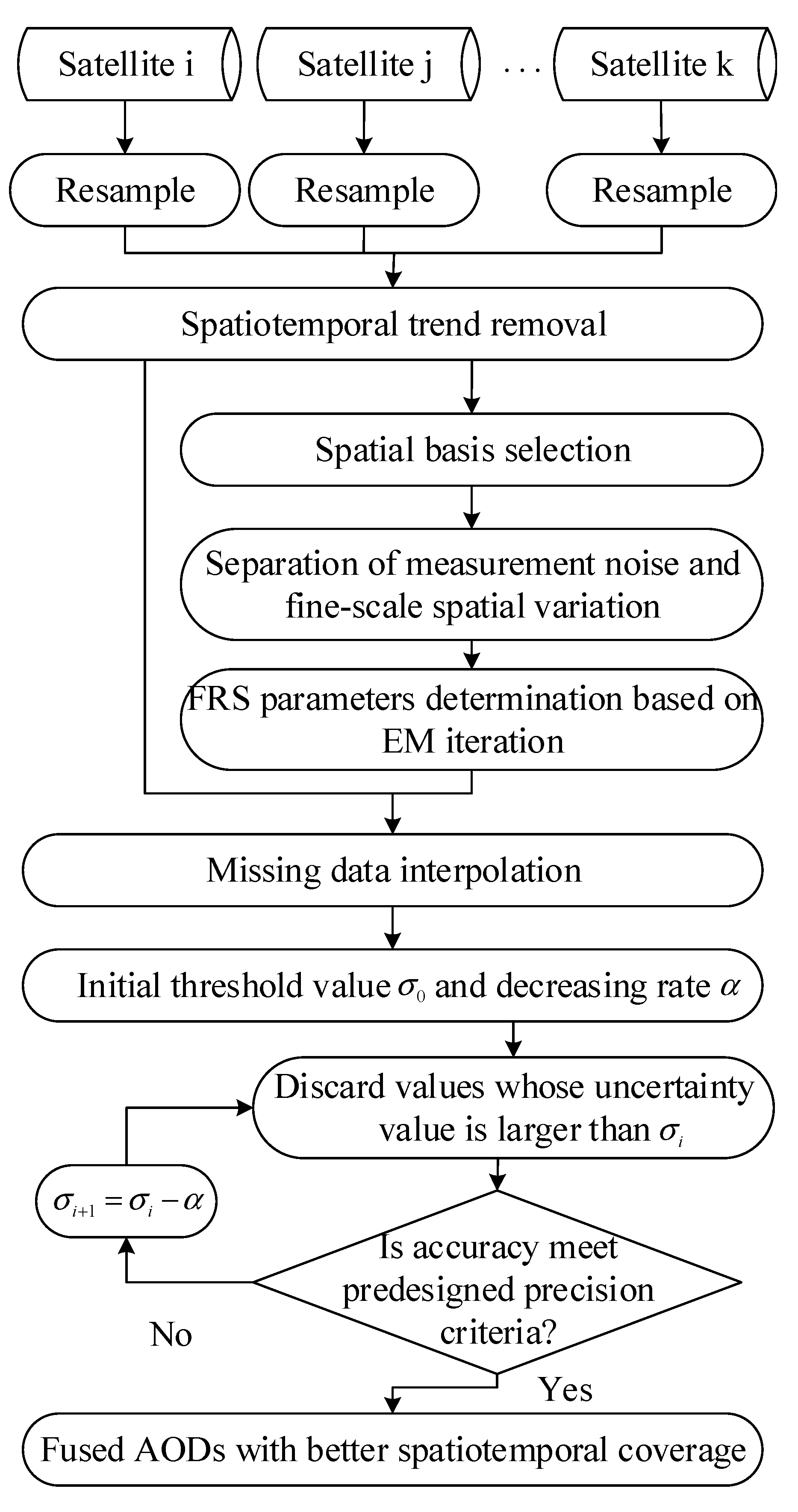
2.2. The FRS-EE Method for AOD Product Fusion

As the FRS method has been thoroughly developed, the basic principle of FRS-EE is similar to FRS. However, by contrast, FRS-EE is designed for a multiple stack AOD products process rather than the one stack in FRS. Moreover, an uncertainty constraint is also introduced by FRS-EE to remove inaccurate AOD estimations. A general process for fusing AOD products from different satellite sensors is demonstrated in Figure 1.
For different satellite AOD dataset fusion, the estimation of real AOD values, Y ( s , t ) , from satellite observations, i.e., Z s a t , i , Z s a t , j and Z s a t , k , is the interest we focused on. In this way, the combined FRS-EE observation equation can be first defined as Equation (6) by stacking AOD products from different satellite sensors in terms of spatial dimension as follows:
( Z s a t , i Z s a t , j Z s a t , k ) t = ( μ s a t , i μ s a t , j μ s a t , k ) t + ( S s a t , i S s a t , j S s a t , k ) η t + ( ξ s a t , i ξ s a t , j ξ s a t , k ) t + ( ε s a t , i ε s a t , j ε s a t , k ) t ,
where μ s a t , i , μ s a t , j , and μ s a t , k are the spatiotemporal trends for Z s a t , i , Z s a t , j , and Z s a t , k at time t , respectively. S s a t , i , S s a t , j , S s a t , k , and ξ s a t , i , ξ s a t , j , ξ s a t , k , as well as ε s a t , i , ε s a t , j , ε s a t , k are the corresponding spatial basis matrices, fine-scale spatial variation vectors, and corresponding measurement noises, respectively.
Then, by considering the temporal connections of AOD products from different satellite sensors as illustrated in Equation (4), the FRS-EE can be further defined as:
( Z s a t , i Z s a t , j Z s a t , k ) t = ( μ s a t , i μ s a t , j μ s a t , k ) t + ( S s a t , i S s a t , j S s a t , k ) η t + ( ξ s a t , i ξ s a t , j ξ s a t , k ) t + ( ε s a t , i ε s a t , j ε s a t , k ) t , η t = Φ t η t 1 + ζ ( t )
According to Figure 1 and Equations (1)–(7), resampling is required due to the specific resolution of different AOD products. Then, the spatiotemporal moving window is employed to remove the spatiotemporal trend μ t , and the spatial basis function S t ( s ) can be selected from multiresolution aspects (see details in Section 3.3). After that, the measurement noise variance σ ε 2 parameter is extracted by fitting the semi-variogram function [23] and the rest of the parameters (i.e., σ ξ 2 , Φ t , U t ) of FRS-EE are obtained by the Expectation-Maximum (EM) estimation [24]. Based on the estimation of parameters ( σ ε 2 , σ ξ 2 , Φ t , U t ), the Kalman smooth method can be utilized to estimate the state vector η t and fine-scale spatial variation ξ ( s , t ) for t = { 1 , 2 , , T } . Afterwards, the AOD values at any spatiotemporal point ( s 0 , t 0 ) and associated uncertainty value can be estimated by FRS-EE using Equations (2) and (3). Considering the high uncertainty of interpolated AOD values in areas without valid satellite AOD observations in both space and time, a threshold criteria-based uncertainty constraint for FRS-EE can be finally introduced to remove the overestimated or underestimated AOD values.

3. Datasets and FRS-EE Model Building

To test the reliability of FRS-EE in effectively and efficiently fusing AOD products from different satellite sensors, this study selected AOD products from Terra-MODIS and Terra-MISR in China (note: the territorial sea is not included in this study) from 2016 to 2017 as a case. Details about the data collection and usage for FRS-EE model building are as follows.

3.1. Dataset Collection

3.1.1. Satellite AOD Products

Satellite AOD products used in this study were collected from MODIS and MISR sensors in the Terra satellite, which ensures that AOD values are retrieved at the same time. AOD products from the MODIS sensor include the 10 km Deep Blue data (DB, Deep_Blue_Aerosol_Optical_Depth_550_Land, Collection 6.0, Level 2) [25] and the 10 km DT_DB_Combined data (AOD_550_Dark_Target_Deep_Blue_Combined, Collection 6.0, Level 2) [26] from the Terra-MODIS sensor (https://ladsweb.modaps.eosdis.nasa.gov). For the DB AOD data, only those with quality assurance (QA) values equal to 2 or 3 are kept [27]. This step is also implemented for the DT_DB_Combined AOD data with QA = 3 [28]. Although the DT_DB_Combined data is the initially fused data combining the DB and Dark Target (DT) data based on the Normalized Difference Vegetation Index (NDVI) data [26], the coverage of the DB data is still higher than the DT_DB_Combined data. For the purpose of improving coverage, the DB data was also adopted in the fusion study. Meanwhile, the AOD data (4.4_KM_PRODUCTS/Aerosol_Optical_Depth, MIL2ASAE, Level-2, Stage 2 and 3 Validated) [29] retrieved with multi angular and multi spectral algorithm [30] from the MISR sensor at a 4.4 km resolution are also considered (https://eosweb.larc.nasa.gov/project/misr/mil2asae_v3). All the satellite AOD products utilized in this study are at the wavelength of 550 nm.

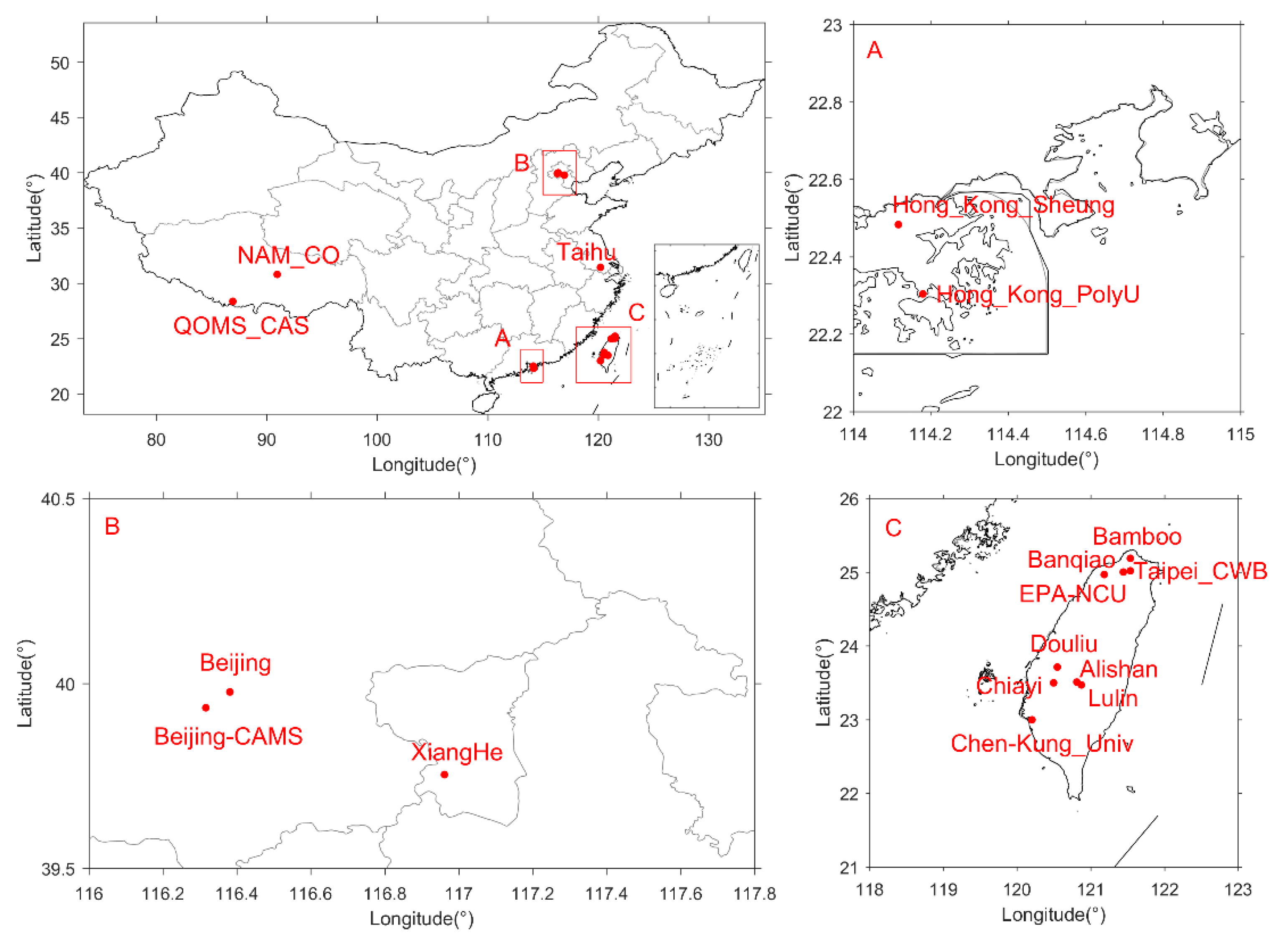
3.1.2. Ground AERONET Data

Ground AERONET sites (https://aeronet.gsfc.nasa.gov/) provide accurate AOD measurements with an uncertainty of 0.01~0.02 [31] and can be used as a benchmark for AOD product validation. Based on the observed AERONET AOD data (Version 3 and Level 2.0) [32] and considering the wavelength of satellite AOD products, this study thus derived AERONET AOD at a 550 nm wavelength by interpolating AOD values at 500 nm and 675 nm using the Ångström exponent distribution assumption [33]. Figure 2 shows the study area and locations of the ground AERONET sites used in this study.

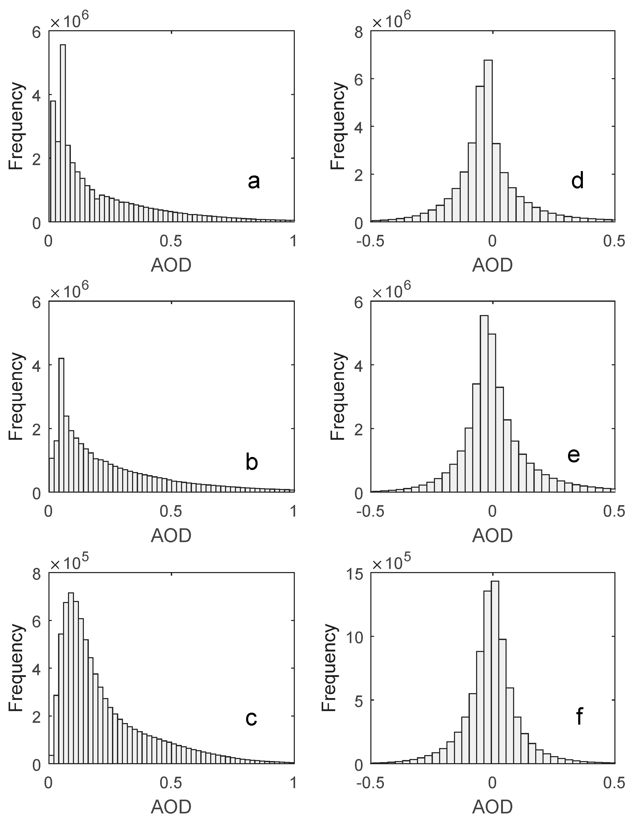
3.2. Spatiotemporal Trend Removal

First of all, we resampled the MISR product at 10 km resolution to match the AOD image pixels of MODIS product. Then, spatiotemporal trend removal was implemented for FRS-EE-based AOD fusion. As shown in Figure 3a–c, the original AOD product histograms from MODIS and MISR are right-skewed, and this does not satisfy the required assumption of a mean of zero and Gaussian distribution for υ ( s , t ) ; hence, the spatiotemporal trend, μ t ( s ) , in Equation (7) should, therefore, be peeled off first for the FRS-EE method. In this process, the average AOD values were first computed by combing AOD products either from MODIS or MISR, pixel by pixel. That is to say, valid AOD retrievals from MODIS and MISR in the same pixel location were averaged. Then, in order to estimate the spatiotemporal trend μ t ( x , y ) at each pixel ( x , y ) of t day, a spatiotemporal moving window with the size of 49 × 49 × 3 was defined according to Tang et al.’s work [20]. After that, the μ t ( x , y ) of the combined AOD data was calculated by averaging AOD values within the spatiotemporal moving window using the following equation:
μ t ( x , y ) = ( i = 24 i = 24 j = 24 j = 24 k = 1 k = 1 A O D ( x + i , y + j , t + k ) ) / N
where N is the number of pixels with available AOD values within each spatiotemporal moving window. The spatiotemporal moving window goes through all pixels until their spatiotemporal trends are calculated. Here, we assume the calculated μ t ( x , y ) based on the spatiotemporal moving window technology is deterministic, and the detrended AOD data for three AOD products from MODIS and MISR sensors can be obtained through the subtraction between original AOD products to the corresponding averaged spatiotemporal trends in each pixel, respectively. It was found that the histograms of three detrended AOD data in Figure 3d–f are approximately Gaussian distributed and have means of zero which demonstrates the calculated spatiotemporal trend μ t ( x , y ) is useful.

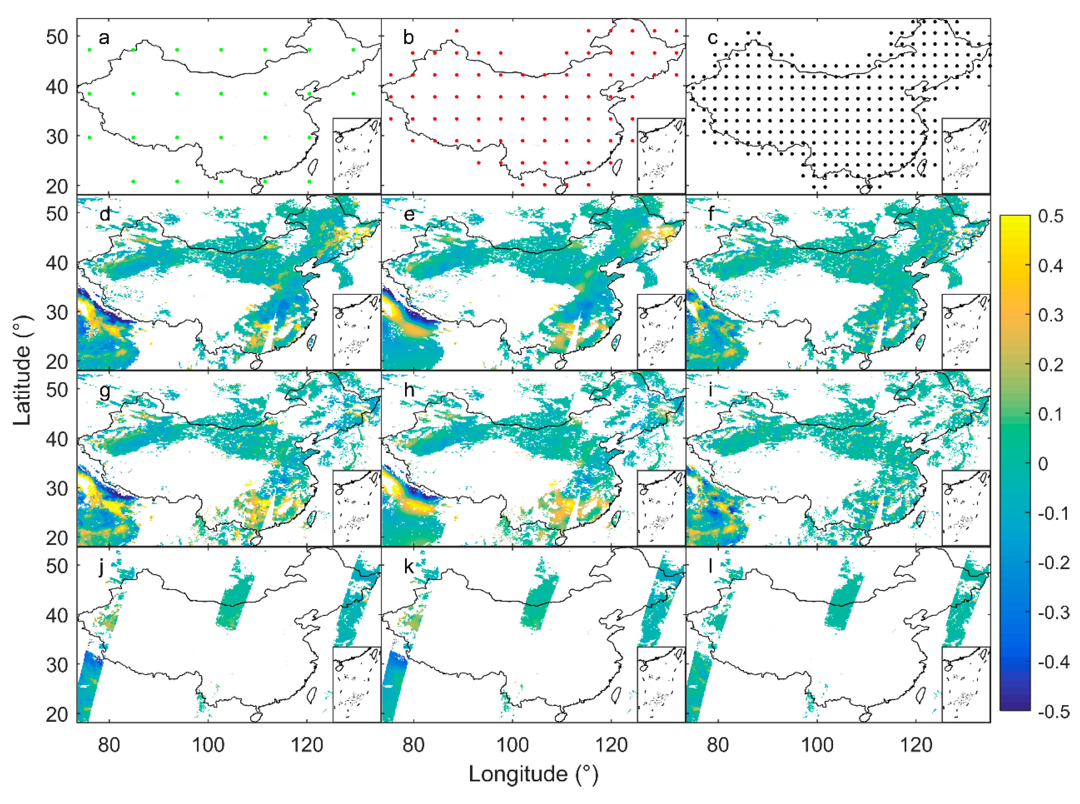
3.3. Selection of Spatial Basis

Spatial basis selection is a very important process aiming to grasp spatial variations in the detrended AOD data. This would greatly ensure that the spatial variations of detrended AOD values are as few as possible denoted by ξ ( s , t ) with the inaccurate spatiotemporally uncorrelated assumption. To date, the functions widely used for spatial basis selection include the smoothing spline basis function, wavelet basis function, bisquare basis function, and radial basis function [23]. Among them, the bisquare basis function has a lot of desirable advantages. For example, it has a clear center point and range, supports different distance types, and can evaluate covariance between any two points in the defined spatial domain [24]. Based on this, the employed bisquare basis function in this study is defined below:
S l ( s ) = { { 1 ( || s c l || / g l ) 2 } 2 || s c l || < g l 0 o t h e r w i s e ,
where c l is the center point location in the l th resolution, and the spatial basis weight S l ( s ) in the c l will be the maximum, i.e., 1. || || is the operator to calculate distance between the s point and the c l center point. g l is the range for the l th resolution, and it is 1.5 times as large as the shortest distance among center points in the l th resolution [23].
In order to obtain the spatial variation at a maximum level, the spatial basis number (i.e., r ) is often chosen at multiple resolutions [23]. The spatial basis with larger resolutions can grasp more global spatial variation, and the spatial basis with finer resolution can grasp more local spatial variation. However, since the computational complexity of the whole FRS method is positively correlated with r cubed (i.e., O ( n T r 3 ) , n is the observation number, and T is study time period) [18], more spatial bases would inevitably increase the cost of FRS-EE in computation time and computer storage. To effectively and efficiently fuse the AOD products from MODIS and MISR, this study attempted to determine spatial bases from a coarse to a fine resolution until a stable residual was obtained after ordinary least square fitting. The residual resi ( s , t ) can be calculated as follows:
d μ t ( s ) = A O D t ( s ) μ t ( s ) ς ( s , t ) = S ( s ) ( ( S ( s ) S ( s ) ) 1 S ( s ) d μ t ( s ) ) resi ( s , t ) = d μ t ( s ) ς ( s , t ) ,
where d μ t ( s ) is the detrended AOD extracted in Section 3.2, ς ( s , t ) is the spatial variation fitted by the spatial basis function of detrended AOD d μ t ( s ) , and resi ( s , t ) is the residual.
We uniformly selected 26 spatial bases in the first resolution, 79 spatial bases in the second resolution, and 293 spatial bases in the third resolution covering the study region, where a total of 398 spatial bases were implemented. Figure 4a–c shows the spatial base center points, i.e., c l in Equation (9), for the first, second, and third resolution, respectively. We can clearly see the center points in the third resolution are closer each other compared with the center points in the first and second resolution. Some spatial base center points were positioned outside the study area on purpose of improving the interpolation accuracy of AOD values near the edge of the study area. Meanwhile, Figure 4d,g,j shows the detrended AOD spatial distribution, i.e., d μ t ( s ) in 30 October 2017 for three satellite AOD products as an example. Figure 4e,h,k shows the fitting effect, i.e., ς ( s , t ) , by three resolution spatial bases which demonstrate that the selected spatial bases determined at the three resolutions can effectively determine the spatial variation from three satellite detrended AODs in Figure 4d,g,j. The residuals, i.e., resi ( s , t ) , in Figure 4f,i,l are also stable, and only a little spatial variation is reserved in the study region, which confirms the selected spatial bases is effective and suitable.

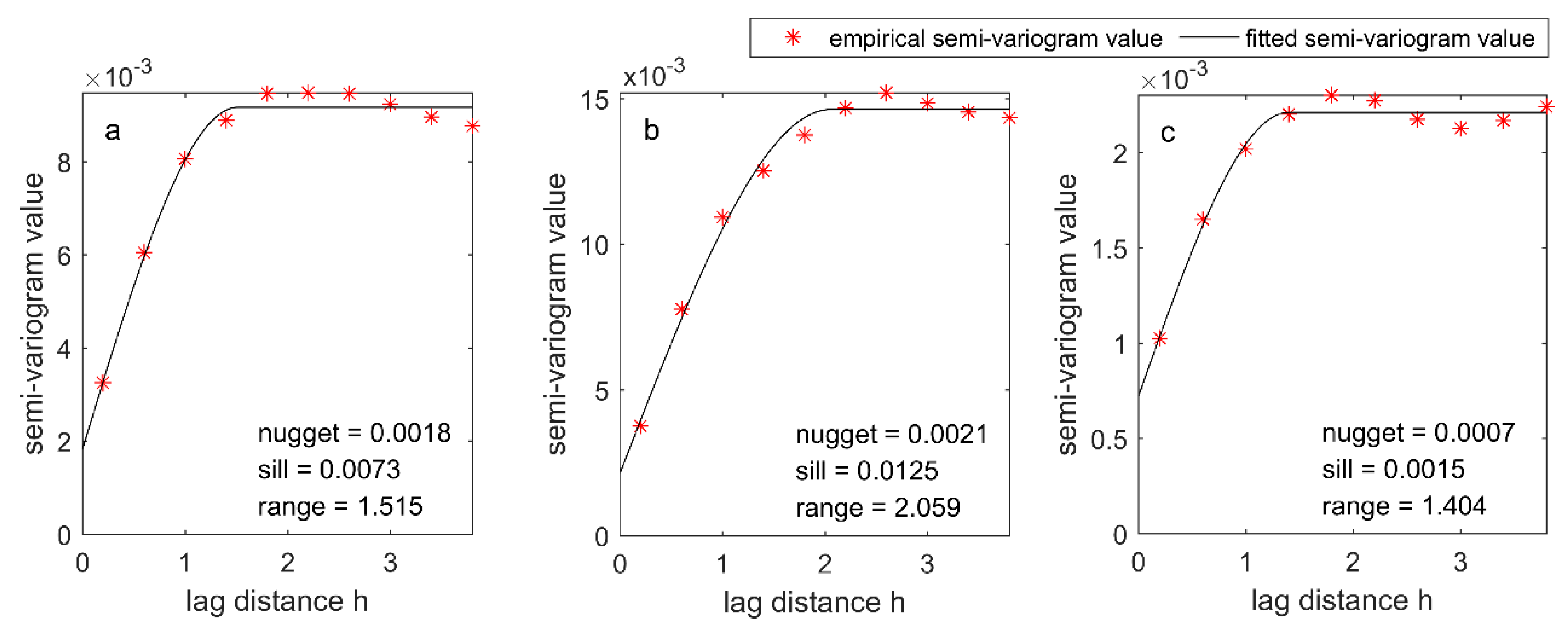
3.4. Separation of Measurement Noise and Fine-Scale Spatial Variation

The residual in Figure 4f,i,l still displays a little spatial variation which can be modeled as the fine-scale spatial variation ξ ( s , t ) . In order to separate measurement noise ε ( s , t ) , and fine-scale spatial variation ξ ( s , t ) in the residual resi ( s , t ) , the semi-variogram function can be adopted under the assumption of spatiotemporal uncorrelated measurement noise ε ( s , t ) and spatial correlated fine-scale spatial variation ξ ( s , t ) [22]. Based on this, the semi-variogram function with spherical model can be used to fit resi ( s , t ) according to Oliver et al. (2014) [34]. Following this, the fitted nugget and sill values of the semi-variogram function are the corresponding σ ε 2 v t ( s ) and σ ξ 2 ν t ( s ) , respectively.
To further calculate the detailed values of nugget and sill of the spherical model in this study, it was assumed that noise variance, σ ε 2 v t ( s ) , is homogeneous in the spatiotemporal domain (i.e., v t i ( s i ) = v t j ( s j ) = 1 ), and fine-scale spatial variation variance, σ ξ 2 ν t ( s ) , is homogeneous in the spatial domain, but heterogeneous in the temporal domain (i.e., ν t ( s i ) = ν t ( s j ) = ν t ). Then, MODIS DB, DT_DB_Combined, and MISR AOD products over 10 days with better spatial coverage were randomly chosen and employed. In this process, the nugget values ( σ ¯ ε 2 ) and sill values ( σ ¯ ξ 2 ) were estimated by averaging their corresponding values over 10 days for each different satellite AOD product as shown in Table 1. The averaged nugget values ( σ ¯ ε 2 ) can be viewed as the variance of uncorrelated spatial variation, i.e., σ ε 2 . The averaged sill values can be used for the variance of correlated spatial variation, i.e., σ ξ 2 , which is also the initial value of the EM iteration in Section 3.5. Figure 5 shows an example of the fitted spherical model and related parameters from 30 October 2017.

3.5. Determination of FRS-EE Parameters Using EM Iteration

Although the Kalman smooth method can estimate η t and ξ ( s , t ) [18], parameters for FRS-EE, i.e., σ ξ 2 , Φ t , U t , and η 0 ~ N ( η 0 | 0 , P 0 | 0 ) , should be known before implementing it. For simplification, we assume Φ t and U t are constant over the temporal domain. Consequently, the EM iteration combined with Kalman smooth would be effective to obtain the maximum likelihood estimates of FRS-EE parameters using a coordinate descent method [24]. Meanwhile, considering the sensitivity of EM iteration to the initial values of FRS-EE parameters, strategies for the parameters’ initialization have to be determined.
For the initial state vector parameter η 0 | 0 with its covariance matrix P 0 | 0 , the first 30 days of detrended AOD values with the least amount of missing data were employed to determine η 0 | 0 and P 0 | 0 using the ordinary least squares method. The averaged sill value σ ¯ ξ 2 was calculated in Section 3.3 as the initial value of σ ξ 2 to indicate the fine-scale spatial variation variance.
For the state transition matrix Φ , a target temporal dependence matrix was first defined [18]:
T 0 = ρ Γ ,
where ρ is a temporal-dependence parameter and was set as 0.95. Γ is the observation covariance matrix and can be described using a semi-variogram model or covariance function. However, due to the large dimension of Γ and its associated great storage requirement resulting from the massive remote sensing AOD datasets in this study, Γ was assumed to be a diagonal matrix, i.e., Γ = ( σ ¯ ξ 2 + σ ^ ε 2 ) I . Based on this, Φ can be obtained by minimizing the following Frobenius norm [18]:
|| S Φ K S diag ( S K S ) 1 / 2 T 0 diag ( S K S ) 1 / 2 ||
where K is a state vector covariance matrix and was also calculated by minimizing the following Frobenius norm [23]:
|| S K S Γ ||
Following Equation (13), the variance matrix U of the state transition error vector ζ ( t ) can be finally calculated by minimizing the Frobenius norm between S U S and 3 Γ to indicate the possible inaccurate assignment for Φ .

3.6. Missing Data Interpolation and Inaccurate Data Removal

Following the steps in Figure 1, any AOD value at spatiotemporal point { s i , t i } that we are interested in can be estimated (i.e., initial FRS fused AOD) after the determination of FRS-EE parameters using EM iteration [24]. Then an uncertainty constraint mechanism for inaccurate interpolated AOD values was implemented to generate the FRS-EE fused AOD. Specifically, an initial threshold value σ 0 (i.e., 0.02) and a decreasing rate α (i.e., 0.0001) were set first. Second, a repeatedly decreased process of threshold values (i.e., σ = σ 0 α ) was iteratively employed to discard the interpolated AOD data with uncertainty values larger than the updated σ . The whole iteration process can stop when the validation accuracy in areas without valid satellite AOD observations meet the predesigned precision criteria by comparing AODs measured at ground AERONET sites. The predesigned precision criteria were the absolute mean Bias | B i a s | < 0.05 , correlation coefficient R > 0.8 , and root mean square error RMSE < 0.35 .

4. Results

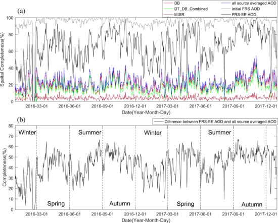
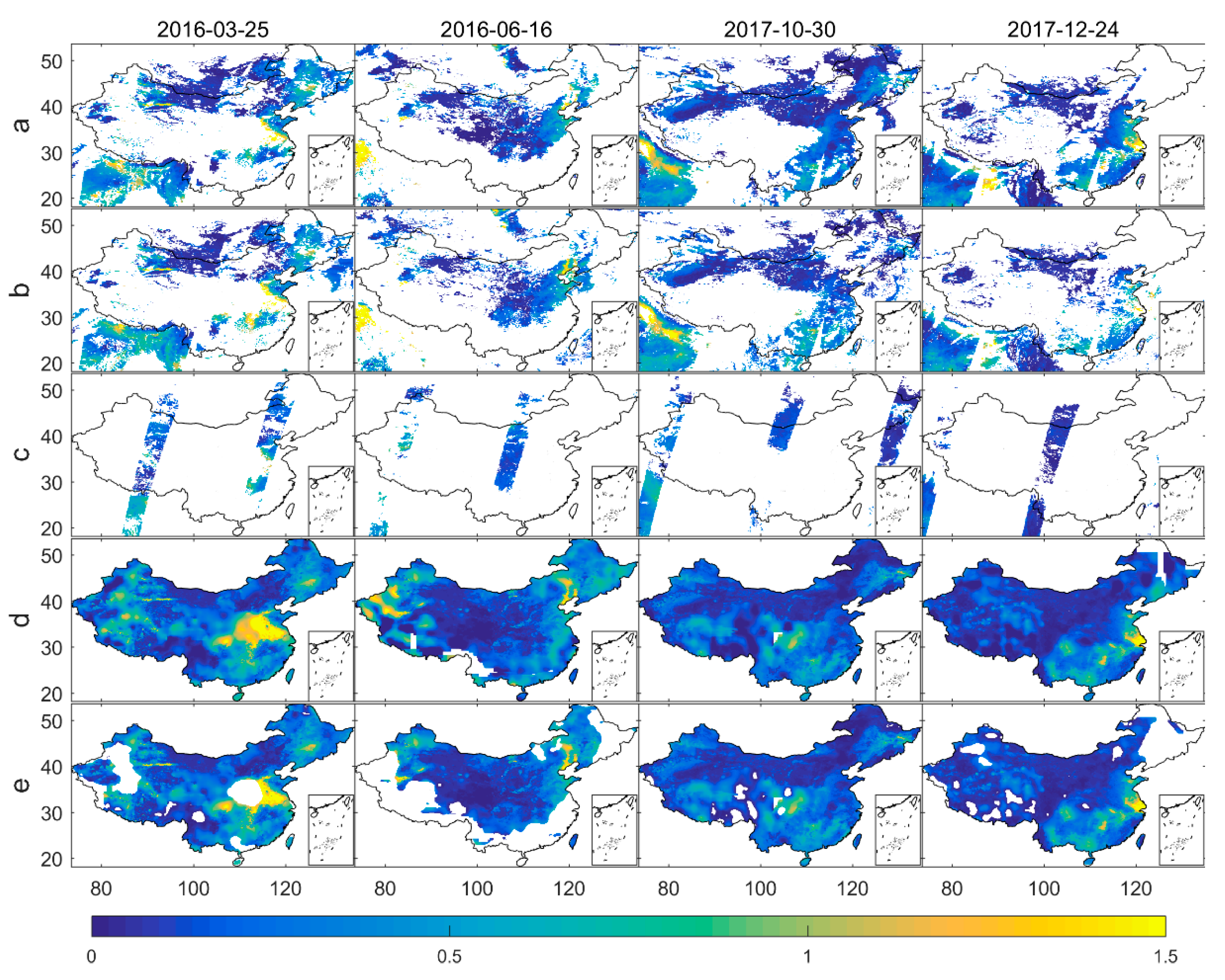
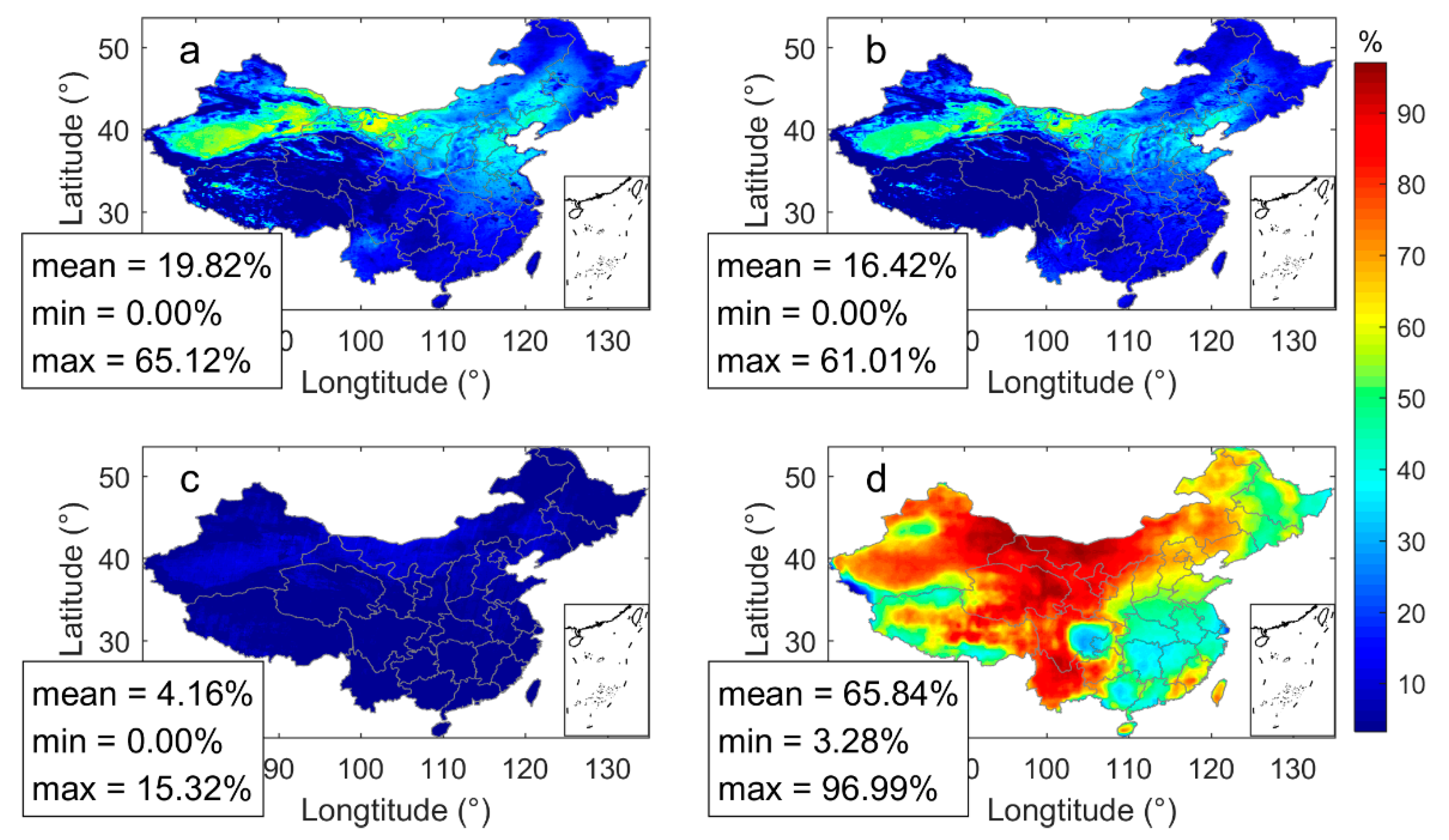
4.1. Spatial Completeness Analysis of Fused AODs

Spatial completeness is one of the most important metrics that can be used to indicate the spatial coverage of satellite-based air pollution monitoring. In this study, spatial completeness is defined as the ratio of the number of grid points with valid satellite AOD values to the total number of grid points over all of China. As illustrated in Figure 6, the spatial completeness of AOD in four typical days across seasons in 2016 and 2017 can be clearly improved by using the FRS-EE method, compared with the original DB AOD, DT_DB_Combined AOD, and MISR AOD. The following daily and seasonal comparison analysis for the spatial completeness of original and fused AODs also further confirmed the effectiveness of FRS-EE in fusing multiple-satellite AODs.
As shown in the comparison of daily spatial completeness in Figure 7, there are significant differences between the original and FRS-EE fused AODs across China over the study period. Among the original DB AOD, DT_DB_Combined AOD, and MISR AOD, the spatial completeness of MISR AOD is the lowest with an average value of 4.16%, while those for DB AOD and DT_DB_Combined AOD are 19.82% and 16.42%, respectively. Although the average daily spatial completeness of single-pixel-based fused AODs (i.e., all source-averaged AOD) is 22.80%, great differences still exist compared to the FRS-EE-based fused AODs. For the initial FRS fused AOD, the average and the maximum daily spatial completeness increased to 95.18% and 100%, respectively. After the removal of the over- and underestimated AODs, the average and the maximum spatial completeness of FRS-EE fused AOD correspondingly reduced to 65.84% and 99.15%, respectively. However, the spatial completeness of these FRS-EE fused AODs are still obviously higher than those of single-pixel-based fused AODs (i.e., daily average improvement: 43.03%, daily maximum improvement: 67.16%). In addition, Table 2 further demonstrates that there are clear seasonal differences for the spatial completeness for the original and FRS-EE fused AODs. Generally, spring and autumn are the seasons with higher spatial completeness for all the original and FRS-EE fused AODs compared with summer and winter. Cloud contamination in summer and snow cover in winter should be responsible for the lower spatial completeness of the original and FRS-EE fused AODs. Similar seasonal improvement effects also occurred for the spatial completeness for the FRS-EE fused AODs. This is reasonable because the FRS-EE fused AODs can borrow strength form more original AODs in spring and autumn but less in summer and winter.

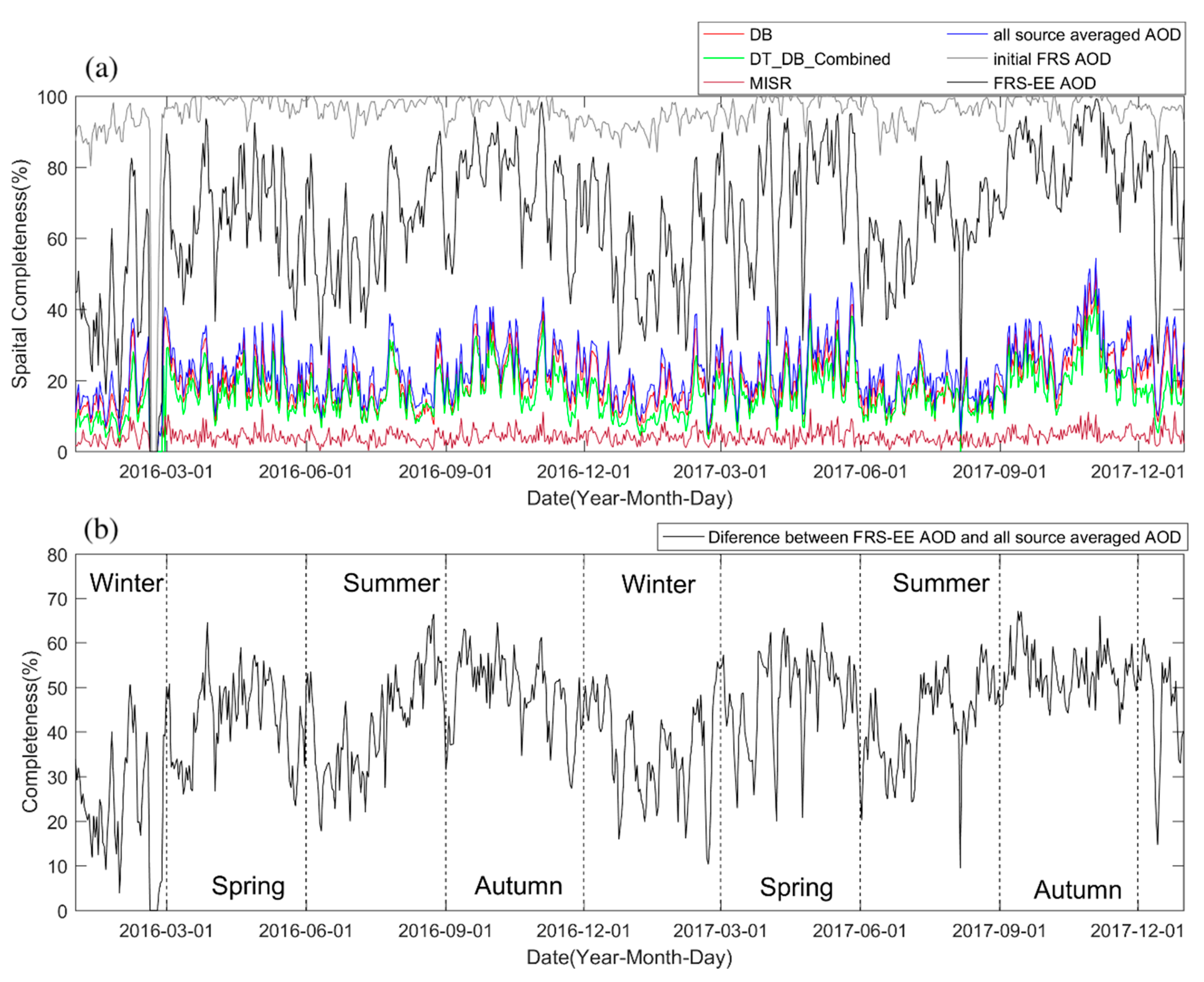
4.2. Temporal Completeness Analysis of Fused AODs

Temporal completeness is an index capable of denoting the repeatable availability of satellite AOD retrievals for a pixel during a particular time period. Similar to the spatial completeness, the temporal completeness in this study is also defined as a ratio, where the number of days with valid satellite AOD values for a pixel are divided by the total days of the entire study period. In this way, the temporal completeness for each pixel across the study area can be calculated. Figure 8 shows spatial differences in temporal completeness for original AOD products and FRS-EE fused AODs. It is clear that the average temporal completeness of DB AOD and DT_DB_Combined AOD is relatively low with mean values of 19.82% and 16.42%, respectively. However, the temporal completeness of these two original AOD products in Xinjiang province is high. The maximum temporal completeness of DB AODs and DT_DB_Combined AODs in Xingjiang is 65.12% and 61.01%, respectively. In contrast, Hongkong is the region with the lowest temporal completeness values of only about 0.67% and 0.94% for DB and DT_DB_Combined AODs, respectively, as it is adjacent to a sea region. For MISR AOD, the temporal completeness is very low, with average and maximum values for all pixels of 4.16% and 15.32%, respectively. Significantly different to the three original satellite AOD products, the temporal completeness of FRS-EE fused AOD is obviously larger, with average and maximum values of 63.39% and 96.58%, respectively. The temporal completeness of FRS-EE fused AODs in the north is large due to the less cloud and high temporal completeness of the original AOD products, which is in contrast to low temporal completeness in the cloudy and rainy southeast region. The low temporal completeness of FRS-EE fused AODs in the Sichuan basin should also be noteworthy. We consider the high spatial heterogeneity of AOD distribution inside and outside Sichuan Basin which result in less strength can be brought from the AODs in the outside Sichuan Basin.
Moreover, Table 3 further shows the average temporal completeness of original satellite AOD products, all source averaged AODs, and FRS-EE fused AODs in different provinces. The location of each province is illustrated in Figure A1. Specifically, the higher average temporal completeness (i.e., greater than 70%) for FRS-EE fused AODs were found in Ningxia, Gansu, Qinghai, Yunnan, Xinjiang, and Neimenggu, while the relatively lower one (i.e., less than 40%) were located in Shanghai province. Compared to the original satellite AOD products and the single pixel based all source averaged AODs, the improvement of temporal completeness for FRS-EE fused AODs is greater than 45% in Qinghai, Yunan, Gansu, Sichuan, Guizhou, Ningxia, Taiwan, and Tibet. In contrast, the regions with relatively weak improvements (i.e., less than 20%) are Shanghai, Anhui, Jiangsu, Henan, and Shandong.

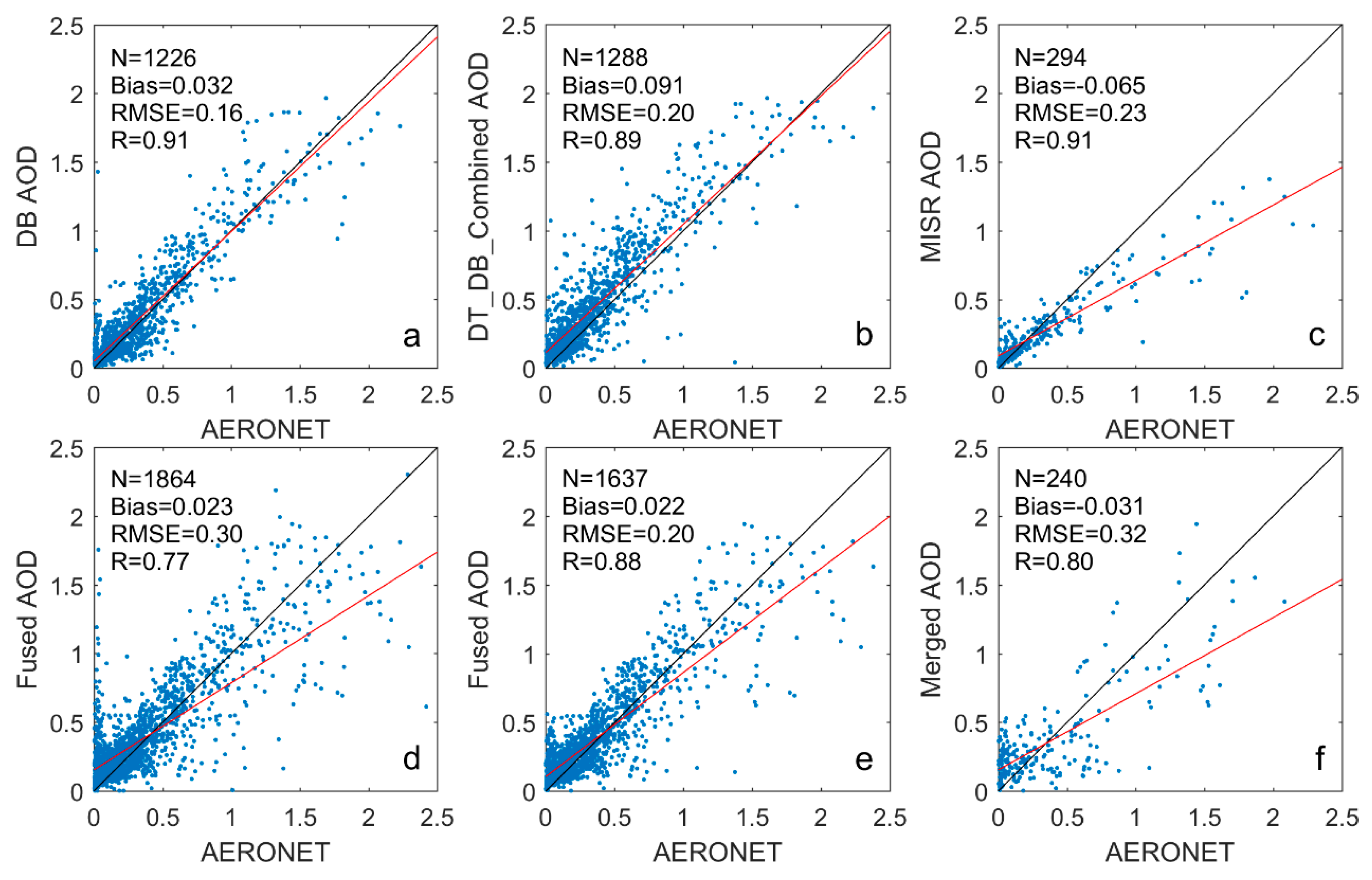
4.3. Accuracy Validation and Time Efficiency Analysis of FRS-EE

To evaluate the accuracy of fused AODs, the original satellite AODs and FRS-EE AODs within 5×5 pixels around the AERONET sites are averaged [35]. Then the measured AODs at the ground AERONET sites within ±30 min of the Terra satellite overpassing time are selected and averaged [36]. In this process, mean bias (Bias), root mean square error (RMSE), and correlation coefficient (R) are employed. Figure 9 shows the validation results of the original satellite AOD products and initial FRS fused and FRS-EE fused AODs with the ground AERONET AOD measurements. Compared to the parameters depicting the accuracy of the original satellite AOD products (i.e., R, 0.91 for DB AOD; R, 0.89 for DT_DB_Combined AOD; R, 0.91 for MISR AOD), the Bias, RMSE, R for initial FRS fused AOD are not ideal, with values of –0.023, 0.30, and 0.77, respectively. However, the FRS-EE fused AOD situation clearly changed with the removal of the overestimated AODs based on the predesigned precision criteria. That is, the Bias, RMSE, R, and within_EE of the FRS-EE fused AOD with uncertainty constraints improved to 0.022, 0.20, and 0.88, respectively. Moreover, as shown in Figure 9f, the accuracy of the FRS-EE fused AODs in grids without any valid satellite AOD inputs are also comparable with those from the original AOD products (Figure 9a–c). Values of Bias, RMSE, and R under this situation are –0.031, 0.32, and 0.80, respectively.
In addition, comparisons of the computation time of FRS-EE and BME under the same computer configuration (i.e., Windows 10 system with 3.00 GHz Intel processor and 128 GB memory) further demonstrated the clear superiority of FRS-EE in fusing the MODIS and MISR AOD products employed across the entire study period. Following the implementation framework of FRS-EE shown in Figure 1, the time cost of spatiotemporal trend removal, spatial base selection, separation of noise and fine-scale spatial variation, EM iteration, spatiotemporal interpolation, and over-/under AODs estimate removal were 2145.96, 11.34, 951.98, 5877.95, 1363.90, and 138.20 s, respectively. That is a total of 2.91 h. However, the time cost of BME in fusing the same AOD products was incomparable, although the experiment was parallelized with a dodeca-core and performed using BMELib (http://www.unc.edu/depts/case/BMELIB/) software. According to the BME based case experiment with AOD data from 9 April 2016, the time cost for soft data construction, spatiotemporal covariance modeling, and spatiotemporal interpolation was 291.78, 387.58, and 111610.50 s, respectively. With the inclusion of the time cost for spatiotemporal trend removal, the total computation time for generating this one-day result under the BME framework was 1.32 days. That would be 30.46 months for two years of data in this study.

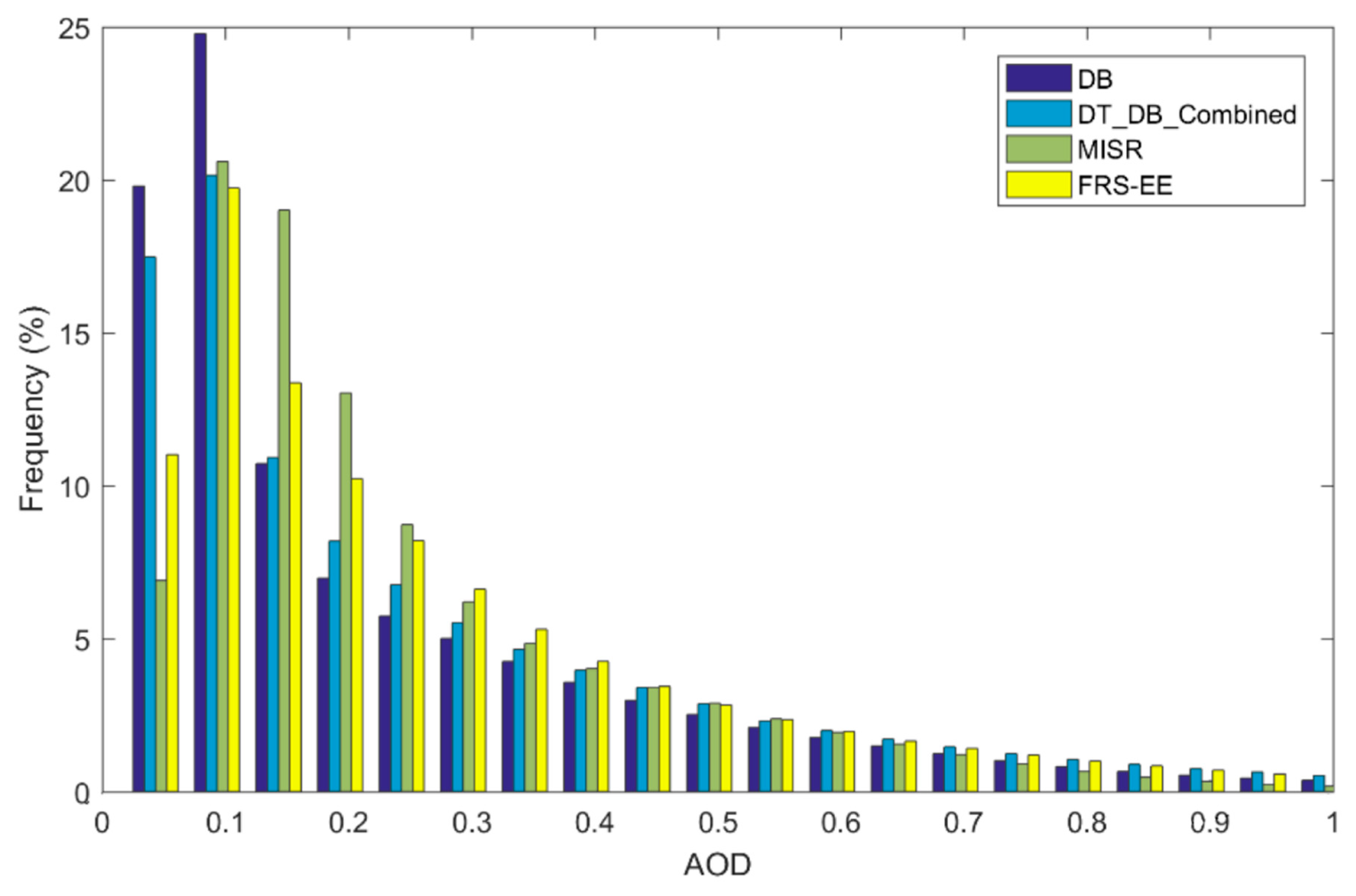
4.4. Overall Effectiveness Analysis of Fused AOD

Figure 10 shows the frequency distribution of AOD values from original DB AOD, DT_DB_Combined AOD, MISR AOD, and FRS-EE fused AOD. Generally, the frequency of the four types of AOD over the study period experienced very similar declining variation, with AOD values larger than 0.1. For AOD values between 0 to 0.1, their frequency inversely increased at the same time. Meanwhile, the asymmetric frequency distribution in Figure 10 also confirms the total histogram of FRS-EE. For FRS-EE fused AOD, the frequency of AOD values between 0 and 1 is 97.18%, and this is very close to the values from DB, DT_DB_Combined, and MISR AODs (i.e., 96.80%, 96.54%, 99.50%, respectively).
Moreover, comparisons of season averaged AODs in Figure 11 further demonstrate the effectiveness of FRS-EE fused AOD in detecting the extreme AOD values with better spatial coverage. While the relatively high AOD values in the Beijing-Tianjin-Hebei region, Xinjiang province, and Sichuan Basin (i.e., spring of 2016 and summer of 2017) can be fully captured by the FRS-EE fused AOD, the seasonal spatial pattern of the FRS-EE fused AOD is very similar to that from the original DB AOD, DT_DB_Combined AOD, and MISR AOD.

5. Discussion

In terms of fusion accuracy, compared with the initial FRS fused results without uncertainty constraints, the FRS-EE fused method using uncertainty constraint to discard some outliers generated in the initial FRS method significantly improved the fusing accuracy from R = 0.77, RMSE = 0.30, and Bias = 0.023 to R = 0.88, RMSE = 0.20, and Bias = 0.022. The discarded AODs mostly occurred in regions far away from all the valid original satellite AODs in the spatiotemporal domain and in regions frequently contaminated with cloud in the temporal domain. The FRS-EE method will assign large uncertainty values for these AODs to discard them. In clear regions surrounded by clouds, although the satellite retrieval algorithm fails to work, the AERONET sites can provide accurate reference AODs to validate the FRS-EE performance, i.e., Figure 9f. However, in those cloudy regions that have valid satellite AODs in the previous or subsequent days, although the AERONET retrieval algorithm cannot work, the FRS-EE still can provide the uncertainty values to diagnose the result reliability. In addition, in regions where all of three satellite AOD products are available, the FRS-EE fused method may generate the AODs with similar performance compared with the original AOD products due to small differences for the estimated measurement noise variance, i.e., σ ε 2 , of three satellite products by the semi-variogram function. The assumption of the semi-variogram method is that the noise is spatiotemporally uncorrelated, and the fine-scale spatial variation is spatially correlated. In the future, the retrieval uncertainty for each AOD product can be used in the estimation of noise variance.
Meanwhile, since the computational complexity for the whole FRS-EE fusion method is O ( n T r 3 ) , the computation time cost of FRS-EE in this study is highly efficient. That is to say, the computational complexity of the FRS-EE method is only cubic with the small spatial basis number r , linear with the observation number n , and study time period T . This allows FRS-EE to process AODs from multiple satellite sensors over large geographic areas and long time series. In this study, the computation time cost for FRS-EE is obviously less than BME (i.e., 2.91 h vs. 30.46 months for two-year AOD data); it can be reduced further, by half, with a little accuracy loss once the Kalman filter is utilized [18]. This might urge the development of automatically and intelligently fused AOD products in the future. However, theoretically, the BME method may generate more accurate fusion results compared with the standard FRS model because the FRS model eliminates some component of spatial variation to improve the computational efficiency [18]. Thus, the BME fusion method is still a reasonable choice if the computation cost is not a concern, i.e., better machine or small dataset. However, as a spatiotemporal fusion method, the BME method will also produce some inaccurate values in a serious missing region [20]. We also recommend the users consider the uncertainty constraint in the BME fusion method as the FRS-EE method does.
Mathematically, the FRS-EE method can be applied in any region. However, the performance of the FRS-EE method may be limited in regions with fewer satellite overpasses, as fewer data may be obtained from the pervious and the next days. Furthermore, similar to previous reported FRS, negatively estimated AOD values are also a problem with FRS-EE, although these negative values only exist in areas without valid satellite AOD retrievals, and many of them can be discarded under the uncertainty constraint of FRS-EE. Future improvements could be focused on the inequality constraints of the FRS equation and the consequent inequality-constrained Kalman filter to produce the directly positive AOD values. Moreover, it is well known that satellite AOD products usually have different spatial and temporal resolutions (i.e., Terra/Aqua-MAIAC 1 km/1 day, Himawari-8 5 km/10 min) due to the difference in aerosol retrieval algorithms and satellite designs (i.e., polar orbit and geostationary satellite). Fusing these different satellite AOD products may be one solution to generate high spatiotemporal AOD data. However, for the FRS-EE method, in order to improve the efficiency, the fixed spatial basis function may bring smoothing effects on high spatial resolution data. Setting more spatial basis functions in a finer resolution with a higher time cost is the solution to this problem. Furthermore, the constant state propagator matrix used in this study also allows the same overpass time of the source satellite data, and adopting a time-varying state propagator matrix will increase the complexity of the method. Thus, the FRS-EE method to generate fused AOD products simultaneously with high spatiotemporal resolution by integrating the temporally and/or spatially independent AOD data is still problematic. In addition, with the termination of old satellite missions, currently reported AOD fusion methods with performance validated based on out-of-date data need to be further confirmed by adopting the AOD products from new satellite missions (i.e., Sentinel-5, Gaofen-5). Finally, in the future, it might also be helpful to introduce ground measurements (i.e., AERONET, CARSNET, AEROCAN, AGSNET, SKYNET, meteorology, land cover, DEM, NDVI, population density) and other related factors regarding AOD emergence, emission, and transition into the spatiotemporal fusion process to produce AODs with higher accuracy and greater coverage. Moreover, the proposed FRS-EE method can still be validated using artificially generated data to test the stability and sensitivity.

6. Summary

In summary, we proposed a newly spatiotemporal fusion method, i.e. FRS-EE, for multiple-satellite AOD products in improving the coverage of AOD data. Compared with the standard FRS and BME, FRS-EE can improve accuracy of FRS by using uncertainty constraints and is more efficient than the time-consuming BME method. Moreover, with the fusion of MODIS DB/DT_DB_Combined AODs and MISR AODs, the FRS-EE method clearly enhances the application of satellite remote sensing for air quality monitoring by generating more spatiotemporally completed AODs.

Author Contributions

Conceptualization, B.Z. and N.L.; methodology, N.L.; validation, N.L.; formal analysis, B.Z., N.L., H.F., X.L.; writing—original draft preparation, N.L.; writing—review and editing, B.Z., H.F., X.L., W.W. and Y.L.; funding acquisition, B.Z. All authors have read and agreed to the published version of the manuscript.

Funding

This research was funded by the National Key Research and Development Program of China, grant number 2016YFC0206205 and the National Natural Science Foundation of China, grant number 41871317.

Acknowledgments

We thank NASA for providing satellite MODIS and MISR AOD products and AERONET PIs and their staff for the establishment and maintenance of AERONET sites. We also thank the UNC-BMElab at the University of North Carolina at Chapel Hill for providing the BMELib MATLAB programs.

Conflicts of Interest

The authors declare no conflict of interest.

Appendix A

Figure A1. The location map of different provinces in China.
Remotesensing 12 01102 g0a1

References

  1. Dominici, F.; Greenstone, M.; Sunstein, C.R. Particulate Matter Matters. Science 2014, 344, 257–259. [Google Scholar] [CrossRef] [PubMed] [Green Version]
  2. Zou, B.; Li, S.; Lin, Y.; Wang, B.; Cao, S.; Zhao, X.; Peng, F.; Qin, N.; Guo, Q.; Feng, H.; et al. Efforts in reducing air pollution exposure risk in China: State versus individuals. Environ. Int. 2020, 137, 105504. [Google Scholar] [CrossRef]
  3. Li, S.X.; Zou, B.; Fang, X.; Lin, Y. Time series modeling of PM2.5 concentrations with residual variance constraint in eastern mainland China during 2013–2017. Sci. Total Environ. 2020, 710, 135755. [Google Scholar] [CrossRef] [PubMed]
  4. Wang, W.; Mao, F.Y.; Zou, B.; Guo, J.P.; Wu, L.X.; Pan, Z.X.; Zang, L. Two-stage Model for Estimating the Spatiotemporal Distribution of Hourly PM1.0 Concentrations over Central and East China. Sci. Total Environ. 2019, 675, 658–666. [Google Scholar] [CrossRef]
  5. Zou, B.; Pu, Q.; Bilal, M.; Weng, Q.; Zhai, L.; Nichol, J.E. High-Resolution Satellite Mapping of Fine Particulates Based on Geographically Weighted Regression. IEEE Geosci. Remote Sens. Lett. 2016, 13, 495–499. [Google Scholar] [CrossRef]
  6. Zhai, L.; Li, S.; Zou, B.; Sang, H.; Fang, X.; Xu, S. An improved geographically weighted regression model for PM2.5 concentration estimation in large areas. Atmos. Environ. 2018, 181, 145–154. [Google Scholar] [CrossRef]
  7. Kokhanovsky, A.A.; Breon, F.-M.; Cacciari, A.; Carboni, E.; Diner, D.; Di Nicolantonio, W.; Grainger, R.G.; Grey, W.M.F.; Höller, R.; Lee, K.-H.; et al. Aerosol remote sensing over land: A comparison of satellite retrievals using different algorithms and instruments. Atmos. Res. 2007, 85, 372–394. [Google Scholar] [CrossRef]
  8. Mélin, F.; Zibordi, G.; Djavidnia, S. Development and validation of a technique for merging satellite derived aerosol optical depth from SeaWiFS and MODIS. Remote Sens. Environ. 2007, 108, 436–450. [Google Scholar] [CrossRef]
  9. Xu, H.; Guang, J.; Xue, Y.; de Leeuw, G.; Che, Y.H.; Guo, X.J.; He, W.; Wang, T.K. A consistent aerosol optical depth (AOD) dataset over mainland China by integration of several AOD products. Atmos. Environ. 2015, 114, 48–56. [Google Scholar] [CrossRef]
  10. Guo, J.; Gu, X.; Yu, T.; Cheng, T.; Chen, H.; Xie, D. Trend analysis of the aerosol optical depth over China using fusion of MODIS and MISR aerosol products via adaptive weighted estimate algorithm. In Proceedings of the SPIE 8866, Earth Observing Systems XVIII, 88661X, San Diego, CA, USA, 23 September 2013. [Google Scholar]
  11. Xue, Y.; Xu, H.; Guang, J.; Mei, L.; Guo, J.; Li, C.; Mikusauskas, R.; He, X. Observation of an agricultural biomass burning in central and east China using merged aerosol optical depth data from multiple satellite missions. Int. J. Remote Sens. 2014, 35, 5971–5983. [Google Scholar] [CrossRef]
  12. Liu, H.; Pinker, R.T.; Holben, B.N. A global view of aerosols from merged transport models, satellite, and ground observations. J. Geophys. Res. Atmos. 2005, 110, D10S15. [Google Scholar] [CrossRef] [Green Version]
  13. Bilal, M.; Nichol, J.E.; Wang, L. New customized methods for improvement of the MODIS C6 Dark Target and Deep Blue merged aerosol product. Remote Sens. Environ. 2017, 197, 115–124. [Google Scholar] [CrossRef]
  14. Bilal, M.; Qiu, Z.; Campbell, J.R.; Spak, S.N.; Shen, X.; Nazeer, M. A new MODIS C6 dark target and Deep Blue merged aerosol product on a 3 km spatial grid. Remote Sens. 2018, 10, 463. [Google Scholar] [CrossRef] [Green Version]
  15. Chatterjee, A.; Michalak, A.M.; Kahn, R.A.; Paradise, S.R.; Braverman, A.J.; Miller, C.E. A geostatistical data fusion technique for merging remote sensing and ground-based observations of aerosol optical thickness. J. Geophys. Res. Atmos. 2010, 115, D20207. [Google Scholar] [CrossRef] [Green Version]
  16. Wang, J.; Brown, D.G.; Hammerling, D. Geostatistical inverse modeling for super-resolution mapping of continuous spatial processes. Remote Sens. Environ. 2013, 139, 205–215. [Google Scholar] [CrossRef]
  17. Nguyen, H.; Cressie, N.; Braverman, A. Spatial Statistical Data Fusion for Remote Sensing Applications. J. Am. Stat. Assoc. 2012, 107, 1004–1018. [Google Scholar] [CrossRef]
  18. Cressie, N.; Shi, T.; Kang, E.L. Fixed Rank Filtering for Spatio-Temporal Data. J. Comput. Graph. Stat. 2010, 19, 724–745. [Google Scholar] [CrossRef] [Green Version]
  19. Yang, J.; Hu, M. Filling the missing data gaps of daily MODIS AOD using spatiotemporal interpolation. Sci. Total Environ. 2018, 633, 677–683. [Google Scholar] [CrossRef]
  20. Tang, Q.; Bo, Y.; Zhu, Y. Spatiotemporal fusion of multiple satellite aerosol optical depth (AOD) products using Bayesian maximum entropy method. J. Geophys. Res. Atmos. 2016, 121, 4034–4048. [Google Scholar] [CrossRef] [Green Version]
  21. Christakos, G. Modern Spatiotemporal Geostatistics, 2nd ed.; Oxford University Press: Oxford, UK, 2008; pp. 260–261. [Google Scholar]
  22. Kang, E.L.; Cressie, N.; Shi, T. Using temporal variability to improve spatial mapping with application to satellite data. Can. J. Stat. 2010, 38, 271–289. [Google Scholar] [CrossRef]
  23. Cressie, N.; Johannesson, G. Fixed Rank Kriging for Very Large Spatial Data Sets. J. R. Statist. Soc. B. 2008, 70, 209–226. [Google Scholar] [CrossRef]
  24. Katzfuss, M.; Cressie, N. Spatio-temporal smoothing and EM estimation for massive remote-sensing data sets. J. Time Ser. Anal. 2011, 32, 430–446. [Google Scholar] [CrossRef]
  25. Sayer, A.M.; Hsu, N.C.; Bettenhausen, C.; Jeong, M.J. Validation and uncertainty estimates for MODIS Collection 6 “Deep Blue” aerosol data. J. Geophys. Res. Atmos. 2013, 118, 7864–7872. [Google Scholar] [CrossRef] [Green Version]
  26. Sayer, A.M.; Munchak, L.A.; Hsu, N.C.; Levy, R.C.; Bettenhausen, C.; Jeong, M.J. MODIS Collection 6 aerosol products: Comparison between Aqua’s e-Deep Blue, Dark Target, and “merged” data sets, and usage recommendations. J. Geophys. Res. Atmos. 2014, 119, 13965–13989. [Google Scholar] [CrossRef]
  27. Hsu, N.C.; Jeong, M.-J.; Bettenhausen, C.; Sayer, A.M.; Hansell, R.; Seftor, C.S.; Huang, J.; Tsay, S.-C. Enhanced Deep Blue aerosol retrieval algorithm: The second generation. J. Geophys. Res. Atmos. 2013, 118, 9296–9315. [Google Scholar] [CrossRef]
  28. Levy, R.C.; Mattoo, S.; Munchak, L.A.; Remer, L.A. The Collection 6 MODIS aerosol products over land and ocean. Atmos. Meas. Tech. 2013, 6, 2989–3034. [Google Scholar] [CrossRef] [Green Version]
  29. Garay, M.J.; Kalashnikova, O.V.; Bull, M.A. Development and assessment of a higher-spatial-resolution (4.4 km) MISR aerosol optical depth product using AERONET-DRAGON data. Atmos. Chem. Phys. 2017, 17, 5095–5106. [Google Scholar] [CrossRef] [Green Version]
  30. Diner, D.J.; John, V.M.; Ralph, A.K.; Bernard, P.; Nadine, G.; David, L.N.; Brent, N.H. Using angular and spectral shape similarity constraints to improve MISR aerosol and surface retrievals over land. Remote Sens. Environ. 2005, 94, 155–171. [Google Scholar] [CrossRef]
  31. Eck, T.F.; Holben, B.N.; Reid, J.S.; Dubovik, O.; Smirnov, A.; O’Neill, N.T.; Slutsker, I.; Kinne, S. Wavelength dependence of the optical depth of biomass burning, urban, and desert dust aerosols. J. Geophys. Res. Atmos. 1999, 104, 31333–31349. [Google Scholar] [CrossRef]
  32. Giles, D.M.; Sinyuk, A.; Sorokin, M.G.; Schafer, J.S.; Smirnov, A.; Slutsker, I.; Eck, T.F.; Holben, B.N.; Lewis, J.R.; Campbell, J.R.; et al. Advancements in the Aerosol Robotic Network (AERONET) Version 3 database—Automated near-real-time quality control algorithm with improved cloud screening for Sun photometer aerosol optical depth (AOD) measurements. Atmos. Meas. Tech. 2019, 12, 169–209. [Google Scholar] [CrossRef] [Green Version]
  33. Ångström, A.; Annaler, G. On the atmospheric transmission of Sun radiation and on dust in the air. Geogr. Ann. 1929, 2, 156–166. [Google Scholar]
  34. Oliver, M.A.; Webster, R. A tutorial guide to geostatistics: Computing and modelling variograms and kriging. Catena 2014, 113, 56–69. [Google Scholar] [CrossRef]
  35. Ichoku, C.; Chu, D.A.; Mattoo, S.; Kaufman, Y.J.; Remer, L.A.; Tanré, D.; Slutsker, I.; Holben, B.N. A spatio-temporal approach for global validation and analysis of MODIS aerosol products. Geophys. Res. Lett. 2002, 29, 1616. [Google Scholar] [CrossRef] [Green Version]
  36. Tao, M.; Chen, L.; Wang, Z.; Tao, J.; Che, H.; Wang, X.; Wang, Y. Comparison and evaluation of the MODIS Collection 6 aerosol data in China. J. Geophys. Res. 2015, 120, 6992–7005. [Google Scholar] [CrossRef]
Figure 1. The flowchart of fusion process of aerosol optical depth (AOD) products from different satellite sensors based on the effective and efficient enhanced fixed rank smooth (FRS-EE) method.
Remotesensing 12 01102 g001
Figure 2. Study area and the locations of ground Aerosol Robotic Network (AERONET) sites.
Remotesensing 12 01102 g002
Figure 3. Histograms of (a) original Deep Blue (DB) AODs, (b) original Dark Target (DT)_DB Combined AODs, (c) original Multiangle Imaging SpectroRadiometer (MISR) AODs, (d) detrended DB AODs, (e) detrended DT_DB_Combined AODs, (f) detrended MISR AODs.
Remotesensing 12 01102 g003
Figure 4. An example of fitting effects with spatial bases under three resolutions in 30 October 2017. Subgraphs (a), (b), and (c) show the spatial base center point locations for the first, second, and third resolution, respectively. Subgraphs (d), (g), and (j) show the detrended DB AOD, detrended DT_DB_Combined AOD, and detrended MISR AOD, respectively. Subgraphs (e), (h), and (k) show the fitting effects with spatial bases under three resolutions, respectively. Subgraphs (f), (i), and (l) are the corresponding residuals, respectively.
Remotesensing 12 01102 g004
Figure 5. An example of fitted semi-variogram function with spherical model for (a) DB AOD residuals, (b) DT_DB_Combined AOD residuals, and (c) MISR AOD residuals in 30 October 2017.
Remotesensing 12 01102 g005
Figure 6. Spatial distributions of (a) DB AOD, (b) DT_DB_Combined AOD, (c) MISR AOD, (d) initial FRS fused AOD, (e) FRS-EE fused AOD in 25 March 2016, 16 June 2016, 30 October 2017, and 24 December 2017 from four seasons during 2016 and 2017, respectively.
Remotesensing 12 01102 g006
Figure 7. Spatial completeness in temporal variation. (a): daily spatial completeness for DB AOD, DT_DB_Combined AOD, MISR AOD, all source averaged AOD, initial FRS fused AOD, and FRS-EE fused AOD. (b): Spatial completeness improvement in each day.
Remotesensing 12 01102 g007
Figure 8. Spatial differences of pixel-level temporal completeness for (a) DB AOD, (b) DT_DB_Combined AOD, (c) MISR AOD, and (d) FRS-EE fused AOD.
Remotesensing 12 01102 g008
Figure 9. Validations of original satellite AOD products and FRS-EE fused AODs with ground AERONET AOD measurements: (a) original DB AOD, (b) original DT_DB_Combined AOD, (c) original MISR AOD, (d) initial FRS fused AOD, (e) FRS-EE fused AOD, (f) FRS-EE fused AOD in areas without valid satellite retrievals.
Remotesensing 12 01102 g009
Figure 10. Frequency distribution for DB AOD, DT_DB_Combined AOD, MISR AOD, and FRS-EE fused AOD.
Remotesensing 12 01102 g010
Figure 11. Season averaged AODs for original DB AOD, DT_DB_Combined AOD, MISR AOD, and FRS-EE fused AOD. MAM: March-April-May; JJA: June-July-August; SON: September-October-November; DJF: December-January-February.
Remotesensing 12 01102 g011
Table 1. Parameters of fitted spherical models for randomly chosen 10 days’ AOD products with better spatial coverage.
DateDBDT_DB_CombinedMISR
NuggetSillNuggetSillNuggetSill
3 November 20170.0020.0100.0030.0100.0010.002
5 November 20170.0020.0090.0020.0080.0020.002
30 October 20170.0020.0070.0020.0120.0010.001
4 November 20170.0030.0100.0020.0080.0010.001
25 May 20170.0020.0050.0030.0060.0010.002
26 May 20170.0030.0040.0020.0060.0020.001
29 October 20170.0020.0090.0020.0120.0010.002
27 October 20170.0030.0110.0030.0130.0010.003
16 May 20170.0010.0050.0020.0040.0020.003
1 November 20170.0020.0100.0030.0100.0010.002
Averaged0.00220.0080.00240.00890.00130.0019
Table 2. Seasonal statistics of the spatial completeness for original, all source averaged, and FRS-EE fused AODs (unit: %). MAM: March-April-May; JJA: June-July-August; SON: September-October-November; DJF: December-January-February.
SeasonMAMJJASONDJF
DB21.49 15.96 25.19 16.66
DT_DB_Combined18.12 14.74 21.16 11.62
MISR4.34 3.54 4.68 4.06
All source averaged AOD24.25 19.65 28.11 19.20
FRS-EE fused AOD69.91 61.59 79.17 52.60
Improvement45.66 41.94 51.05 33.40
Table 3. The average of temporal completeness for original, all source averaged, and FRS-EE fused AODs in different provinces.
ProvinceDBDT_DB_CombinedMISRAll Source AveragedFRS-EE FusedImprovement
Qinghai7.71 4.49 3.01 10.55 81.58 71.02
Yunnan14.76 13.04 2.45 17.92 79.36 61.43
Gansu25.23 20.87 5.30 28.65 86.27 57.63
Sichuan7.84 6.04 2.00 10.73 67.14 56.41
Guizhou7.78 8.05 1.00 9.53 65.65 56.12
Ningxia28.73 25.00 5.65 32.56 86.70 54.14
Taiwan5.19 9.24 1.68 11.19 63.74 52.55
Tibet6.87 3.01 2.70 9.28 61.36 52.08
Fujian11.72 10.70 2.47 14.81 58.64 43.83
Hainan6.49 10.10 1.71 11.58 53.84 42.26
Neimenggu30.90 24.54 6.64 33.95 75.96 42.01
Xinjiang28.29 24.18 5.20 30.47 71.69 41.22
Hongkong0.67 0.94 1.55 2.62 41.98 39.36
Chongqing9.94 10.76 1.42 12.95 50.43 37.48
Shaanxi23.95 23.56 4.05 28.26 64.85 36.59
Guangdong10.62 10.72 2.28 13.48 49.30 35.82
Guangxi9.99 10.53 1.57 12.48 48.06 35.58
Heilongjiang16.87 14.46 3.19 19.90 52.39 32.49
Shanxi28.29 27.08 5.98 33.79 64.91 31.11
Jilin20.27 17.28 4.21 23.93 53.64 29.70
Beijing33.81 31.49 7.74 40.89 68.96 28.07
Tianjin33.81 28.65 7.40 38.37 64.38 26.00
Hebei33.94 29.99 6.58 38.32 64.25 25.93
Zhejiang13.86 12.55 2.43 17.87 43.70 25.83
Liaoning31.31 28.41 6.65 36.11 61.69 25.59
Hunan13.08 11.74 2.37 15.54 40.53 25.00
Jiangxi15.41 13.44 2.95 18.32 42.85 24.53
Hubei18.97 15.95 3.34 22.17 43.29 21.12
Shandong32.04 28.21 5.65 36.75 55.39 18.64
Henan26.89 22.03 4.94 30.46 48.59 18.12
Jiangsu21.86 15.82 4.08 26.00 42.97 16.97
Anhui23.74 17.78 4.60 26.63 43.46 16.83
Shanghai7.16 7.34 1.90 11.17 27.90 16.73

