Improved Detection of Inundation below the Forest Canopy using Normalized LiDAR Intensity Data
by
 , ,
, ,
Megan W. Lang
1, 
Vincent Kim
2,
Gregory W. McCarty
3,*,
Xia Li
3,
In-Young Yeo
4,
Chengquan Huang
5 and
Ling Du
3 1
U.S. Fish and Wildlife Service, 5275 Leesburg Pike, Falls Church, VA 22041, USA
2
National Oceanic and Atmospheric Administration/National Environmental Satellite, Data, and Information Service, 5830 University Research Ct, College Park, MD 20740, USA
3
Hydrology and Remote Sensing Laboratory, USDA-ARS, Beltsville, MD 20705, USA
4
School of Engineering, The University of Newcastle, Callaghan, NSW 2308, Australia
5
Department of Geographical Sciences, University of Maryland, College Park, MD 20742, USA
*
Author to whom correspondence should be addressed.
Remote Sens. 2020, 12(4), 707; https://doi.org/10.3390/rs12040707
Submission received: 31 December 2019
/
Revised: 10 February 2020
/
Accepted: 19 February 2020
/
Published: 21 February 2020
(This article belongs to the Special Issue Wetland Landscape Change Mapping Using Remote Sensing)
Abstract
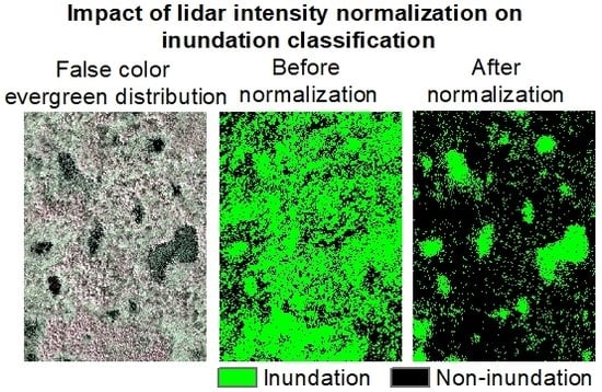
:To best conserve wetlands and manage associated ecosystem services in the face of climate and land-use change, wetlands must be routinely monitored to assess their extent and function. Wetland extent and function are largely driven by spatial and temporal patterns in inundation and soil moisture, which to date have been challenging to map, especially within forested wetlands. The objective of this paper is to investigate the different, but often interacting effects, of evergreen vegetation and inundation on leaf-off bare earth return lidar intensity within mixed deciduous-evergreen forests in the Coastal Plain of Maryland, and to develop an inundation mapping approach that is robust in areas of varying levels of evergreen influence. This was achieved through statistical comparison of field derived metrics, and development of a simple yet robust normalization process, based on first of many, and bare earth lidar intensity returns. Results demonstrate the confounding influence of forest canopy gap fraction and inundation, and the effectiveness of the normalization process. After normalization, inundated deciduous forest could be distinguished from non-inundated evergreen forest. Inundation was mapped with an overall accuracy between 99.4% and 100%. Inundation maps created using this approach provide insights into physical processes in support of environmental decision-making, and a vital link between fine-scale physical conditions and moderate resolution satellite imagery through enhanced calibration and validation.
1. Introduction
For effective landscape management under the context of climate change, wetlands must be routinely monitored to assess extent and function. Since in situ monitoring of wetlands at the landscape scale is typically cost and time prohibitive, remotely sensed data are commonly used to assess wetlands at this spatial scale [1]. Traditionally, optical images, such as aerial photography, in conjunction with field data were used to map wetlands [1]. The U.S. Fish and Wildlife Service National Wetlands Inventory (NWI) data are primarily produced using this approach [1]. Although great care has been taken in the production of these data, and they are relied upon by numerous managers and scientists, challenges to this type of cartographic process remain [1,2,3]. These challenges result in increased uncertainty for certain wetland types, including forested wetlands [2,3]. Palustrine forested wetlands are one of the most difficult types of wetlands to map using optical images [1]. This is in large part because the forest canopy precludes viewing of the ground’s surface, the expression of wetland hydrology is often intermittent, and trees found in this type of wetland are often identical or spectrally similar to those found in upland forests. Forested wetlands are especially difficult to map in areas of low topographic relief, such as the outer Coastal Plain of the Mid-Atlantic U.S. As a result, all forested wetlands, but especially smaller, drier wetlands, are often difficult to detect using optical data [1].
Other types of remotely sensed data are now being used to enhance forested wetland mapping, including synthetic aperture radar (SAR) [4,5] and light detection and ranging (LiDAR or lidar) [6,7] data. Although both SAR and lidar offer unique strengths that have the potential to greatly improve forested wetland mapping [8], the development of natural resource applications involving lidar data has been particularly rapid. The incorporation of lidar data into the wetland mapping process has the potential to improve both the detail and reliability of forested wetland maps [7,8,9]. This paper focuses on discrete point return lidar data [10,11] collected using a near-infrared (i.e., 1064 nm) laser, specifically lidar intensity. Lidar intensity or amplitude is the amount of energy returned to the sensor per lidar echo relative to the amount of energy transmitted by the sensor per laser pulse [12]. Information regarding the processing of lidar intensity data, particularly the calibration of lidar intensity data can be found in Kashani et al. [13].
With the rapid development of lidar technology and increased availability of lidar data, many applications of this dataset have not been fully developed [11]. This is particularly true for lidar intensity data. Intensity data have been used for land cover classification, and are especially useful when different land covers have distinct levels of reflectance in the portion of the electromagnetic spectrum detected by the sensor. Most lidar intensity studies have focused on forestry (e.g., tree species identification) [14,15,16,17,18,19] and other types of vegetation related applications [16,17,19,20,21,22,23,24], but the use of lidar intensity to identify other materials is slowly increasing (e.g., [land cover including asphalt roads, grass, house roofs, and trees] [25], [sediment quality relative to the potential to preserve archaeological materials] [26], [agricultural land use classes] [27], and [building footprints] [28]). A few studies have used lidar intensity data along with other inputs to map aquatic and coastal ecosystems [12,29,30,31,32,33] with mixed outcomes (i.e., lidar intensity was only sometimes determined to be helpful for this application). Only a couple of studies have examined the ability of lidar intensity data to map inundation below the forest canopy, especially relatively small discontinuous areas of inundation [34,35,36,37]. We are not aware of any studies that have considered the influence of forest structure on the ability to map inundation below the forest canopy using lidar intensity.
In an earlier study, Lang and McCarty [37] found that lidar intensity data were well suited for the identification of inundation below the forest canopy due to the strong absorption of incident near-infrared energy by water and the ability to isolate bare earth returns from vegetation canopy returns. The objective of this subsequent study is to investigate the different, but often similar, effects of evergreen vegetation and inundation on leaf-off bare earth return lidar intensity within mixed deciduous-evergreen forests, and to develop an inundation mapping approach that is robust in areas of varying levels of evergreen influence. We hypothesize that the intensity of returns from the forest canopy can be used to identify and correct for the influence of the forest canopy on the intensity of bare earth returns. Improved maps of forested wetland inundation can be used to: 1) assess ecosystem character at a fine spatial resolution for the prediction of ecosystem function and provision of related ecosystem services, and 2) allow for enhanced calibration and validation of inundation maps based on coarser spatial resolution remotely sensed data. Indeed, highly accurate relatively fine spatial resolution maps provide a critical link between in situ information and moderate spatial resolution imagery. These fine spatial resolution products can be used to support the development of broad-scale land cover maps using a variety of input datasets and techniques (e.g., machine learning or deep learning models using a wide variety of image types including high spatial or temporal resolution satellite images), even when only available over relatively small areas. However, before these fine spatial resolution datasets are used to support mapping at a coarser spatial resolution, efforts should be made to reduce errors arising from the presence of evergreen vegetation. The research described herein supports the development of more rapid and reliable operational wetland mapping within forested environments.
2. Materials and Methods
2.1. Study Site
The 33 km2 study site (Figure 1) is located within the headwaters of the Choptank River watershed. The 1756 km2 Choptank River watershed is located on the Delmarva Peninsula within the outer Coastal Plain Physiographic Province. The Choptank River is a major tributary of the Chesapeake Bay, originating in Kent County, Delaware and flowing southwest towards its outlet near Cambridge, Maryland. The area is characterized by a temperate climate with average annual precipitation of 120 cm [38]. About half of annual precipitation is lost to the atmosphere via evapotranspiration, while the remainder recharges groundwater or enters streams via surface flow [38]. The landscape is relatively flat (max elevation <30 m above sea level) and land cover is dominated by farmland (~60%) with smaller amounts of forest (33%) and suburban/urban (7%) area [39]. Within the study area, approximately 4% of forests are evergreen [37], and evergreen tree species primarily include loblolly pine (Pinus taeda L.), Virginia pine (Pinus virginiana Mill.), and American holly (Ilex opaca Aiton).
Roughly 50% of the forested area within the Choptank River watershed is wetland. The most common types of wetlands found within the study area are wetland depressions (e.g., Delmarva bays) and flats, with a smaller area of riparian wetlands. Most wetlands are inundated or saturated early in the growing season, with some wetlands remaining inundated well into the summer. The period of maximum hydrologic expression (i.e., highest groundwater levels and most area inundated) varies with antecedent weather conditions, but is typically in or around March when evapotranspiration has been relatively low for a long period of time, relative to other months, and before evapotranspiration increases markedly with rising temperatures and forest canopy leaf-out. The primary soil types within forested areas at the study site are Hammonton-Fallsington-Corsica complex (predominantly moderately well drained), Corsica mucky loam (predominantly very poorly drained), and Fallsington sandy loam (predominantly poorly drained) in order from most to least common (Natural Resources Conservation Service Soil Survey Geographic Database https://gdg.sc.egov.usda.gov).
2.2. Lidar Data Collection and Preprocessing
Lidar intensity data were collected over the study area on 27 March, 2007 and 24 March, 2009, by the Canann Valley Institute (see Lang and McCarty [37] for a detailed description of the 2007 lidar dataset). These dates represent both average (2007) and moderate drought (2009) conditions, according to the National Oceanic and Atmospheric Administration (NOAA) Palmer Z Index as calculated over a three-month time period (NOAA National Climate Data Center http://cdo.ncdc.noaa.gov). The data were collected at the beginning of the local growing season as it relates to the definition of wetlands (last −2.2 °C or lower freeze at the 50% probability level for Dover, Delaware is March 28; National Oceanic and Atmospheric Administration National Climate Data Center http://cdo.ncdc.noaa.gov), and within the approximate average period of maximum hydrologic expression. It is during the spring when wetland water levels are typically at their highest [37]. Precipitation did not occur for at least four days before lidar data acquisitions. Therefore, field data collected within a couple days of image acquisition should represent conditions during the lidar collection. Twelve cm spatial resolution true color digital aerial imagery were collected by the Canann Valley Institute synchronously with the 2009 lidar data.
On 27 March, 2007, lidar data were collected using an Optech Airborne Laser Terrain Mapper (ALTM) 3100 sensor (1064 nm wavelength laser) with a scan angle of +/−20° at a height of 610 m above the Earth’s surface with a pulse rate of 100,000 Hz and scan frequency of 50 Hz. On 24 March, 2009, lidar data were collected using the same sensor, altitude, and pulse rate with a scan angle of +/−10° and a scan frequency of 70 Hz. For each laser pulse, the instrument recorded up to four returns. The vertical accuracy of both lidar data acquisitions was validated using over 100 precision global positioning system (GPS) points collected at sites of constant elevation (e.g., parking lots and road intersections) using a Trimble Real-Time Kinematic (RTK) 4700 GPS/base station combination and a Maryland State Highway Administration surveyed benchmark. The lidar data had an overall vertical accuracy of ~0.15 m root-mean-square error (RMSE) and an average point density of ~2.5 pts/m2 (0.40 m post spacing) and ~11 pts/m2 (0.09 m post spacing), for the 2007 and 2009 datasets, respectively. Horizontal accuracy is expected to be approximately 0.31 m based on sensor specifications (Teledyne Optech, personal communication). Raw data were converted to LASer (LAS) files containing x, y, z, and intensity data. Bare earth returns (i.e., returns from the Earth’s surface with returns from vegetation, buildings, and other elevated features removed) were classified by the data provider using Terrascan v 7.0 software. DASHMap v 4.0027 software (Teledyne Optech, Ontario Canada) was used to range normalize (i.e., correct for variation in signal travel length) the 2009 intensity data. The 2007 intensity data were not range normalized, because variations in intensity due to range (e.g., tonal variations between scan lines) were not evident. The influence of confounding parameters (i.e., factors other than the parameter of interest) was minimized for both dates by collecting data at a study site with minimal topographic variations, using a moderate scan angle to reduce variations due to range [40], and collecting the data over a short time period on a day with no noticeable atmospheric interference (e.g., clouds or haze) to reduce the impact of atmospheric absorption. Inverse distance weighted (IDW) interpolation was used to produce 1 m bare earth and first of many (abbreviated herein as “first”) return lidar intensity raster images. All images were filtered using a median filter with a kernel size of three to reduce fine-scale salt and pepper noise while minimally effecting borders between land cover classes.
2.3. In Situ Data
In situ data were collected within forests at two reserves owned by The Nature Conservancy, which were visited within three days of the 2009 lidar acquisition. No precipitation occurred during this time period. A Trimble 6000 Series GeoXH global positioning system (GPS) was used to collect over 1000 field data points along transects. The Trimble GeoXH GPS was designed to operate under a forest canopy and is capable of collecting data using real-time Wide Area Augmentation System (WAAS) correction. GPS accuracy was enhanced by collecting multiple (>15) GPS readings at each location. The field data points were collected along randomly traversed paths within forested areas, the location of which was partly controlled by accessibility after entering forest patches from random access points. GPS points were collected at least 12 m apart at the center of areas with homogeneous inundation status (i.e., inundated, non-inundated, or transitional between inundated and non-inundated) within an 8 m diameter. The presence or absence of an evergreen canopy was noted at each GPS point. Transitional areas were often found in relatively narrow buffers in between inundated and non-inundated areas, but were only sampled where these areas met or exceeded 8 m in diameter. Gaps are naturally present within forests, but large areas of open canopy were avoided to limit the scope of the study to areas with a forest canopy. GPS points, along with inundation status and tree type (i.e., evergreen or deciduous), were outputted to ArcGIS v 10.2 (ESRI, Redlands, California, USA). A similar process was used to collect in situ data in support of the 2007 collection [37].
2.4. Analysis
2.4.1. Characterization of Lidar Intensity by Land Cover Type
In situ data were used to create frequency distributions for 2007 and 2009 using the bare earth intensity values. Intensity values were extracted for each ground data collection point on the bare earth intensity images, and the frequency of these values was plotted at 5 digital number (DN) intervals for each class, including evergreen, non-inundated deciduous, and inundated deciduous forest. Values for the transitional class were also noted.
The 12 cm digital true-color imagery collected coincident with the 2009 lidar data were used to identify more than ten regions of interest (ROIs) to represent three classes: evergreen, non-inundated deciduous, and inundated deciduous forest. Representative areas were selected as ROIs throughout the study area, and resulted in at least several thousand samples per class. Evergreen forests were examined for indications of inundation, but none were found. This is not surprising since wetlands in the region generally do not support evergreen trees (Whigham D, personal communication). Land cover was verified using aerial photographs collected coincident with the 2007 lidar data [37]. General statistics, including median and mean, as well as 10th, 25th, 75th, and 90th percentiles were extracted from the bare earth and first intensity images for each class and a scatter plot was created to visualize intensity differences between classes.
The relationships between evergreen vegetation as identified using digital true-color imagery collected coincident with the 2009 lidar data and first return lidar intensity, and first return lidar intensity and bare earth return lidar intensity, were quantified using the range normalized 2009 lidar dataset. The relationship between evergreen vegetation as identified using digital true-color imagery and first return intensity was considered first. A total of 74 250 m2 ROIs were created over forested areas with a wide range of percent evergreen canopy. These ROIs were used to sample first return lidar intensity images and a VIgreen vegetation index (green-red/green+red) [41] image created using the digital true-color aerial imagery collected coincident to the 2009 lidar data. The relationship between these datasets was then investigated using simple linear regression. The relationship between first and bare earth lidar returns from a single laser pulse was also characterized for thousands of pulses within mixed deciduous and evergreen forest areas using simple linear regression.
2.4.2. Inundation Map Production
Due to the confounding effects of inundation and evergreen canopy on bare earth intensity, a technique was developed to normalize bare earth images for the presence of evergreen canopy (i.e., gap fraction) while retaining the inundation signal to improve inundation map accuracy and visual clarity (Figure 2). Since the level of energy of earlier returns should be proportional to the energy that is not transmitted through the canopy (see description of Beer–Lambert equation of light extinction in Richardson et al. [42]), we added first return intensity to bare earth intensity across the entire study area to help compensate for the effect of reduced laser transmission with greater canopy cover. To determine the proportion of first return intensity needed to compensate for reduced transmission, we used summary statistics from the previously described evergreen and non-inundated deciduous ROIs and the equation:
where F1 and G1 are the median first and bare earth return intensities for non-inundated deciduous ROIs, and F2 and G2 are the median first and bare earth intensities for non-inundated evergreen ROIs. Thus the normalized bare earth return is equal to C * F + G where C is determined as previously described.
C = (G2 − G1)/(F1 − F2)
This numerical relationship was used to produce a normalized bare earth intensity image for both image dates. Basic statistics including median and mean, as well as 10th, 25th, 75th, and 90th percentiles were extracted from the normalized bare earth image for each of the prior created ROIs (i.e., evergreen, non-inundated deciduous, and inundated deciduous forest classes) and a box plot was created to visualize differences in bare earth intensity between classes. The normalized bare earth images were filtered twice using an enhanced lee filter [43] with kernel sizes of 5 and 7. Maps depicting inundated, non-inundated, and transitional areas were produced for 2007 and 2009 by thresholding the normalized bare earth intensity images. The maximum inundated deciduous ROI value (52.3) and the minimum non-inundated deciduous forest ROI value (59.6) were used as thresholds for the 2009 image. Since greater variability was present in the 2007 data and the inundated and non-inundated classes were not completely distinct, the 99.5th percentile of the inundated deciduous ROI values (82.9) and the 0.5th percentile of the non-inundated ROI values (106.2) were used as thresholds for the 2007 image. Values in between the two thresholds were considered to represent the transitional class.
2.4.3. Inundation Map Characterization and Validation
The effect of normalizing the bare earth intensity images using the approach described above was assessed by creating frequency distributions and error matrices using the in situ data, as well as applying normalized and non-normalized datasets within a maximum likelihood classifier. The ArcGIS spatial analyst “extract values to points” cubic convolution function was used to extract an intensity value for each ground data collection point on the normalized bare earth intensity images and the frequency of these values was plotted at 5 digital number (DN) intervals for each class, including evergreen, non-inundated deciduous, and inundated deciduous forest. Values for the transitional class were also noted. The in situ data were also used to create error matrices for the inundated and non-inundated classes. Transitional areas were not used to support the accuracy assessment due to their relatively low number (35 plots), but are displayed for reference. Finally, to further test the utility of the normalized lidar intensity dataset, the maximum likelihood classifier in ENVI v. 5.5.2 (Harris Geospatial Solutions, Broomfield, Colorado, USA) was used to map inundation using training data created using normalized and non-normalized bare earth lidar intensity data.
3. Results
Before normalization, the bare earth data provided a relatively clear distinction between the inundated and non-inundated deciduous classes for both years, but the evergreen class was difficult to distinguish (Figure 3 and Figure 4). However, within the ROI scatter plots (Figure 4) a clear distinction between the evergreen and inundated deciduous classes was present within the first return data. Note that within class variability is higher for 2007 relative to 2009 and that ranges for each class vary between years.
The presence of evergreen vegetation assessed using true-color aerial imagery collected, coincident to the 2009 lidar data, was found to be well correlated with the strength of the 2009 lidar first returns, while a moderate negative correlation was found between first and bare earth returns. A significant positive linear relationship (r2 of 0.82 [p = < 0.0001]) was found between first returns and the VIgreen vegetation index. A significant negative relationship (r2 of 0.53 [p = < 0.0001]) was found between first and bare earth returns when comparing individual pulses.
The coefficients used to normalize the bare earth lidar intensity were 1.95 and 1.98, for 2007 and 2009, respectively. After these coefficient values were used to normalize bare earth intensity for the influence of the evergreen canopy, a clear distinction between inundated and non-inundated classes was evident (Figure 5).
The shift of evergreen areas to higher bare earth returns after normalization is evident when comparing Figure 3 and Figure 6, as well as Figure 4 and Figure 5. Figure 7 illustrates the influence of first return strength on the original bare earth images, and the dramatic increase in the clarity of inundation boundaries after normalization. Note the similarity in first return images created for the same area using data from 2007 and 2009, but the decrease in inundation present on the landscape during 2009 (drought) relative to 2007 (average). Figure 8 demonstrates that the normalization process resulted in a bare earth image that not only distinguishes inundated from non-inundated deciduous and non-inundated evergreen forest areas from inundated deciduous forest areas, but also maintains transitional areas. These transitional areas are found in areas where it would be logical to find either smaller discontinuous areas of inundation or areas of saturated soils. Transitional areas are often located intermediate between the inundated and non-inundated classes, but are also found on hummocks within inundated areas and along ditches, likely partially due to mixed pixels.
Both inundation maps were found to be highly accurate (Table 1), and by comparing the two maps the effect of antecedent weather conditions on area inundated was evident. Although relatively few transitional data points were sampled in the field and thus accuracy is not reported for this class, the intensity of areas classified as transitional in the field was intermediate to areas classified as inundated and non-inundated in the field. While non-inundated areas appeared relatively bright on the 2009 normalized image (median 78 DN; 10th percentile 66 DN; 90th percentile 89 DN) and inundated areas appeared relatively dark (median 22 DN; 10th percentile 12 DN; 90th percentile 38 DN), transitional areas had an intermediate appearance (median 46 DN; 10th percentile 32 DN; 90th percentile 61 DN). Area inundated during average weather conditions (2007; 3.08 km2), was approximately three times larger than during drought conditions (2009; 1.3 km2). Transitional area was approximately twice as large during average as compared to drought conditions, 2.6 km2 and 1.4 km2, respectively. Ninety-seven percent and 100 % of evergreen areas were mapped as non-inundated during 2007 and 2009, respectively. However, 1 evergreen point was mapped as transitional in 2007, and 4 in 2009.
Two maximum likelihood classifications illustrated substantial differences when trained using maps of inundation based on non-normalized versus normalized lidar intensity data (Figure 9). Although the map trained using the normalized dataset did contain some uncertainty, areas of inundation were clearly visible. On the other hand, the map trained using the non-normalized dataset was dominated by error and areas of inundation were difficult to distinguish from the surrounding evergreen canopy.
4. Discussion
A wide range of lidar intensity calibration has been implemented, and range correction is most commonly applied [13,26,27,28,32,44,45]. However, many scientists decide that calibration is not necessary for their particular application [16,28,35,46,47,48,49]. Due to the visually robust difference between inundated and non-inundated forest and the lack of apparent range effects due to scan angle the 2007 dataset was not range normalized. However, these differences were visually evident in the 2009 dataset so that dataset was corrected for range, which removed within flight line differences. The need for calibration varies markedly based on the intended use of the intensity data [13]. Applications relying on the detection of relatively small variations in intensity and those in certain landscapes (e.g., areas of high topographic variability) or using certain data collection specifications (e.g., larger angles of incidence, acquisitions with divergent specifications or multiple sensors) will likely find calibration to be more important for meeting their objectives [13,26,27,28,35,50].
Multiple authors have mentioned that calibration is complex within forested environments due to the mixed nature of the forest signal [21,27,43,51,52]. Surface roughness and orientation, as well as vegetation structure and density in addition to material composition will affect bare earth returns [13,14,15,16,17,18,19,20,21,22,23,24,25,26,27,28,29,30,31,32,33,34,35,36,37,38,39,40,41,42,43,44,45,46,47,48,49,50]. For this reason, inherent variability in the signal is expected to be high and range normalization may not result in a reduction in signal variation within forest classes [27]. Regardless, we did note a reduction in within class signal variability for the 2009 lidar intensity dataset (range normalized) versus the 2007 dataset (not range normalized; Figure 3 and Figure 4). Range normalization may have reduced within class variability in the 2009 dataset, but it is not vital for production of lidar intensity based inundation maps at our study site; inundation maps based on both datasets were found to be highly accurate when compared to field validation data. This study helps to address one of the four primary knowledge gaps listed by Kashani et al. [13], which include the need to identify the degree of calibration necessary for different applications.
It should be noted that even after range correction, intensity values will vary based on individual sensor specifications (e.g., scan angle and pulse frequency) and other factors [13,34]. Many data acquisition specifications affect intensity values, including some that are not communicated to the end user, thus making absolute calibration of intensity challenging for most data users [13,21,27,44,53]. In addition, lidar sensors have and will continue to be enhanced, which will change specifications further. For this reason and others, the normalization coefficient and inundation classification threshold values presented in this paper would likely not be directly applicable to other datasets. Instead, information on relative values and methods presented in this article can be applied elsewhere. Kim et al. [54] also found that ranges in intensity values for land cover classes varied between lidar intensity datasets, but this did not affect map accuracy.
Our findings regarding the significant negative correlation (r2 = 0.53) between same pulse first and ground returns is not surprising, since the amount of energy returned to the sensor is dependent on a number of variables, including target reflectivity but also area of the laser footprint intercepted. A laser pulse that first intersects the canopy has less energy left when it encounters the forest floor, and the lower gap fraction is within the canopy the less energy will be transmitted through the canopy and potentially made available at the ground surface. This principle has been used to estimate gap fraction [55]. For example, Lefsky et al. [56] suggested that canopy gap fraction could be estimated using a ratio of ground to total returns. Hopkinson and Chasmer [55] found that the ratio of ground to total returns was largely based on gap fraction (r2 = 0.86). Lefsky et al. [56] noted that the relationship between canopy gap fraction and the ratio between ground and total returns should be modified for reflectance properties at the ground and canopy levels. The results of this paper support this assertion.
Presumably based at least in part on variations in gap fraction between evergreen and broadleaved deciduous tree canopies during the leaf-off season, Kim et al. [47] found that leaf-off intensity data could be used to discriminate between broadleaved and evergreen species with an accuracy of 83.4%. The significant linear relationship (r2 = 0.82) between VIgreen, which has been used by others to estimate vegetation fraction [41] which is generally considered to be the inverse of gap fraction [57], and first returns further demonstrates the relationship between gap fraction and the lidar signal.
Kashani et al. [13] list wetness as one of two primary drivers of the lidar intensity signal, and suggest that intensity could be used to remove the influence of wet areas. Others have instead used this signal to map wet areas. Lang and McCarty [37] demonstrated that lidar intensity data could be used to produce highly accurate (97%) maps of inundation below the forest canopy, but hypothesized that evergreen vegetation was a source of error. Stevens and Wolfe [35] also found that lidar intensity could be used to map inundation beneath multiple types of vegetation canopy, including spruce and birch forests, peatlands and fens, with high levels of accuracy (93%). Variation within their dataset was attributed to absorption characteristics and surface roughness. This study expands on past studies by directly quantifying the interacting effects of the forest canopy and inundation, and offering a simple yet robust method to minimize the effects of the forest canopy on derived inundation maps. The higher levels of accuracy reported in this study (Table 1), reflect not only the advantage provided by the capacity to filter lidar data by order of return and the stark contrast between inundated and non-inundated ground when observed using a near-infrared laser, but also the efficacy of the normalization process.
Figure 5 indicates that our approach results in the clear separation of inundated and non-inundated land cover, regardless of forest canopy type (evergreen or deciduous). Figure 6 confirms this assertion using field data. Figure 7 illustrates the effect of the correction method in areas of varying evergreen canopy distributions. Figure 7 also demonstrates that the correction technique not only provides clearer definition of depressional wetland inundation extent, but it also assists in the identification of relatively narrow surface water connections between inundated areas. Surface water connections amongst wetlands and between wetlands and streams have been the focus of recent scientific efforts, in part because these connections have been used to determine wetland jurisdictional status [58,59,60,61]. Duration of connection is an important component of these types of investigations, and will be better supported by lidar intensity data as multi-date lidar become more available in the future.
This study represents an initial investigation into the enhancement of lidar intensity data to better map inundation, but additional research is necessary. For example, processing procedures, including interpolation and filtering are critical to the success of lidar applications, and should be investigated relative to lidar intensity based inundation mapping. In addition, given the relatively large margins between the inundated and non-inundated pixels it may be possible to automate derivation of the threshold map class values (i.e., normalization coefficients) in the future. While further research is needed to develop such automated methods, a similar approach was developed by Huang et al. [62] for identifying dark dense forest pixels automatically. Finally, additional research is needed to better characterize the influence of soil moisture on return intensity. A negative correlation between soil moisture and bare earth intensity has been hypothesized or reported by multiple authors [26,45,63,64,65]. Although our study did not directly address the detection of soil moisture, our results indicate that substantial differences in soil moisture or discontinuous inundation, which is often accompanied by soil saturation, could substantially and predictably affect bare earth returns.
This study both helps to address fundamental knowledge gaps pertaining to the use of lidar intensity data, including the need to evaluate the influence of surface wetness [13], and supports the improved mapping of inundation. Inundation maps produced using lidar intensity data could be used to support the enhanced calibration and validation of inundation maps produced over larger areas a wide variety of image types including high spatial or temporal resolution satellite images. The substantial positive effect of the normalization process on the quality of inundation training data and therefore classification results is illustrated in Figure 9. The importance of this type of foundational study will increase as lidar data are collected over a larger geography, and multi-date lidar data become more readily available.
Although binary inundation status is not the same as wetland status, areas that are inundated at the beginning of the growing season during an average year are very likely to meet the hydrologic definition of a wetland (i.e., inundated or saturated within the root zone for two weeks within the growing season) [66]. Therefore, areas that were mapped as inundated during 2007 are likely to be wetlands, and these maps could be used to improve the mapping of forested wetlands, a wetland class that has proven difficult to map in the past [8]. As reported by Kloiber et al. [67], the initial delineation of wetland boundaries is time consuming. This study further demonstrates that at least some of these boundaries can be produced using highly accurate automated processes, further supporting the assertion made by Kloiber et al. [67].
5. Conclusions
To date, most studies that have used lidar intensity to map specific landscape characteristics have focused exclusively on their primary parameters of interest (e.g., vegetation structure or inundation). Mixed deciduous and evergreen forested wetlands and their surrounding uplands present an ideal location for exploring the interacting effects of canopy structure, inundation, and soil moisture. This study represents an initial step towards a more integrated approach to assessing drivers of the lidar intensity signal within forested landscapes.
The method described herein is relatively simple, highly accurate, and can be achieved using data that are often readily available. Although use of lidar intensity data has increased in recent years, the dataset is still underutilized given its strong potential to benefit a number of applications, including improved mapping of aquatic ecosystems. Furthermore, the pairing of intensity and elevation data is powerful and the fact that lidar intensity are independent from sun shadow, lighting conditions and high level clouds is an additional advantage. All of these factors contributed to the accuracy of our inundation maps. We predict that the use of lidar intensity data to map land cover will become more common as fundamental investigations into use of the intensity signal continue and intensity calibration becomes more robust. This research provides details regarding physical drivers of the lidar intensity signal and presents a method for mapping inundation below the forest canopy that is relatively simple, yet robust.
Author Contributions
M.W.L. is the primary author who collected the data, processed the high-resolution remote sensing datasets, generated results, and wrote the manuscript. V.K. and X.L. supported geospatial analyses. G.W.M. was responsible for the overall design of the work and results interpretation. I.-Y.Y. and C.H. advised on data analyses, modeling, and mapping. L.D. performed landscape modeling. All authors have read and agreed to the published version of the manuscript.
Funding
This research was supported by the wetland component of the Natural Resources Conservation Service Conservation Effects Assessment Project, and the National Aeronautics and Space Administration’s Land Cover and Land Use Change Program (contract No: NNX12AG21G and NNX15AK66G).
Acknowledgments
We greatly acknowledge the cooperation of private landowners, especially The Nature Conservancy. The findings and conclusions in this article are those of the author(s) and do not necessarily represent the views of the U.S. Fish and Wildlife Service. All trade names are included for the benefit of the reader and do not imply an endorsement of or preference for the product listed by the U.S. Department of Agriculture.
Conflicts of Interest
The authors declare no conflict of interest.
Abbreviations
The following abbreviations are used in this manuscript:
| NWI | National Wetland Inventory |
| SAR | Synthetic Aperture Radar |
| LiDAR | Light Detection and Ranging |
| DEM | Digital Elevation Model |
| NOAA | National Oceanic and Atmospheric Administration |
| ALTM | Airborne Laser Terrain Mapper |
| GPS | Global Positioning System |
| RTK | Real-Time Kinematic |
| RMSE | Root-mean-square error |
| LAS | LASer |
| IDW | Inverse Distance Weighted |
| WAAS | Wide Area Augmentation System |
| DN | Digital Number |
| ROI | Region of Interest |
| NiSAR | NASA (National Aeronautics and Space Administration)-ISRO (Indian Space Research Organization) Synthetic Aperture Radar |
References
- Tiner, R.W. Use of high-altitude aerial photography for inventorying forested wetlands in the United States. For. Ecol. Manag. 1990, 33–34, 593–604. [Google Scholar] [CrossRef]
- Stolt, M.H.; Baker, J.C. Evaluation of national wetland inventory maps to inventory wetlands in the southern Blue Ridge of Virginia. Wetlands 1995, 15, 346–353. [Google Scholar] [CrossRef]
- Kudray, G.M.; Gale, G.M. Evaluation of national wetland and inventory maps in a heavily forested region in the upper great lakes. Wetlands 2000, 20, 581–587. [Google Scholar] [CrossRef]
- Lang, M.W.; Kasischke, E.S.; Prince, S.D.; Pittman, K.W. Assessment of C-band synthetic aperture radar data for mapping and monitoring Coastal Plain forested wetlands in the Mid-Atlantic Region, U.S.A. Remote Sens. Environ. 2008, 112, 4120–4130. [Google Scholar] [CrossRef]
- Oliver-Cabrera, T.; Wdowinski, S. InSAR-based mapping of tidal inundation extent and amplitude in Louisiana coastal wetlands. Remote Sens. 2016, 8, 393. [Google Scholar] [CrossRef] [Green Version]
- Lang, M.W.; McCarty, G.W.; Oesterling, R.; Yeo, I.Y. Topographic metrics for improved mapping of forested wetlands. Wetlands 2013, 33, 141–155. [Google Scholar] [CrossRef]
- Vanderhoof, M.K.; Distler, H.E.; Mendiola, D.A.T.G.; Lang, M. Integrating Radarsat-2, Lidar, and Worldview-3 imagery to maximize detection of forested inundation extent in the Delmarva Peninsula, USA. Remote Sens. 2017, 9, 105. [Google Scholar] [CrossRef] [Green Version]
- Lang, M.; Bourgeau-Chavez, L.; Tiner, R.; Klemas, V. Advances in remotely sensed data and techniques for wetland mapping and monitoring. In Remote Sensing of Wetlands: Applications and Advances; Tiner, R., Lang, M., Klemas, V., Eds.; CRC Press: Boca Raton, FL, USA, 2015; pp. 74–112. [Google Scholar]
- Snyder, G.; Lang, M. Significance of a 3D elevation program to wetland mapping. Natl. Wetl. Newsl. 2012, 34, 11–15. [Google Scholar]
- Goodwin, N.R.; Coops, N.C.; Culvenor, D.S. Assessment of forest structure with airborne LiDAR and the effects of platform altitude. Remote Sens. Environ. 2006, 103, 140–152. [Google Scholar] [CrossRef]
- Vierling, K.T.; Vierling, L.A.; Gould, W.A.; Martinuzzi, S.; Clawges, R.M. Lidar: Shedding new light on habitat characterization and modeling. Front. Ecol. Environ. 2008, 6, 90–98. [Google Scholar] [CrossRef] [Green Version]
- Chust, G.; Galparsoro, I.; Borja, Á.; Franco, J.; Uriarte, A. Coastal and estuarine habitat mapping, using LIDAR height and intensity and multi-spectral imagery. Estuar. Coast. Shelf Sci. 2008, 78, 633–643. [Google Scholar] [CrossRef]
- Kashani, A.G.; Olsen, M.J.; Parrish, C.E.; Wilson, N. A review of LIDAR radiometric processing: From ad hoc intensity correction to rigorous radiometric calibration. Sensors 2015, 15, 28099–28128. [Google Scholar] [CrossRef] [PubMed] [Green Version]
- Schreier, H.; Lougheed, J.; Tucker, C.; Leckie, D. Automated measurements of terrain reflection and height variations using an airborne infrared laser system. Int. J. Remote Sens. 1985, 6, 101–446. [Google Scholar] [CrossRef]
- Lim, K.; Treitz, P.; Wulder, M.; St-Ongé, B.; Flood, M. LiDAR remote sensing of forest structure. Prog. Phys. Geogr. 2003, 27, 88–106. [Google Scholar] [CrossRef] [Green Version]
- Holmgren, J.; Persson, Å. Identifying species of individual trees using airborne laser scanner. Remote Sens. Environ. 2004, 90, 415–423. [Google Scholar] [CrossRef]
- Holmgren, J.; Persson, Å.; Söderman, U. Species identification of individual trees by combining high resolution LiDAR data with multi-spectral images. Int. J. Remote Sens. 2008, 29, 1537–1552. [Google Scholar] [CrossRef]
- Zhang, Z.; Liu, X. Support vector machines for tree species identification using LiDAR-derived structure and intensity variables. Geocarto Int. 2013, 28, 364–378. [Google Scholar] [CrossRef]
- Donoghue, D.N.M.; Watt, P.J.; Cox, N.J.; Wilson, J. Remote sensing of species mixtures in conifer plantations using LiDAR height and intensity data. Remote Sens. Environ. 2007, 110, 509–522. [Google Scholar] [CrossRef]
- Kim, S.; Hinckley, T.; Briggs, D. Classifying individual tree genera using stepwise cluster analysis based on height and intensity metrics derived from airborne laser scanner data. Remote Sens. Environ. 2011, 115, 3329–3342. [Google Scholar] [CrossRef]
- Korpela, I.; Hovi, A.; Korhonen, L. Backscattering of Individual Lidar Pulses from Forest Canopies Explained by Photogrammetrically Derived Vegetation Structure. Int. Arch. Photogramm. Remote Sens. Spat. Inf. Sci. 2013, XL-1/W1, 171–176. [Google Scholar] [CrossRef] [Green Version]
- Hancock, S.; Essery, R.; Reid, T.; Carle, J.; Baxter, R.; Rutter, N.; Huntley, B. Photography: An examination of relative limitations. Agric. For. Meteorol. 2014, 189–190, 105–114. [Google Scholar] [CrossRef] [Green Version]
- Su, J.G.; Bork, E.W. Characterization of diverse plant communities in Aspen Parkland rangeland using LiDAR data. Appl. Veg. Sci. 2007, 10, 407–416. [Google Scholar] [CrossRef]
- Zhuang, W.; Mountrakis, G.; Wiley, J.J.; Beier, C.M. Estimation of above-ground forest biomass using metrics based on Gaussian decomposition of waveform lidar data. Int. J. Remote Sens. 2015, 36, 1871–1889. [Google Scholar] [CrossRef]
- Song, J.-H.; Han, S.-H.; Yu, K.; Kim, Y.-I. Assessing the possibility of land-cover classification using lidar intensity data. Int. Arch. Photogramm. Remote Sens. Spat. Inf. Sci. 2002, 34, 259–262. [Google Scholar]
- Challis, K.; Carey, C.; Kincey, M.; Howard, A.J. Assessing the preservation potential of temperate, lowland alluvial sediments using airborne lidar intensity. J. Archaeol. Sci. 2011, 38, 301–311. [Google Scholar] [CrossRef]
- Mesas-Carrascosa, F.J.; Castillejo-González, I.L.; De la Orden, M.S.; Porras, A.G.F. Combining LiDAR intensity with aerial camera data to discriminate agricultural land uses. Comput. Electron. Agric. 2012, 84, 36–46. [Google Scholar] [CrossRef]
- Zhao, T.; Wang, J. Use of lidar-derived NDTI and intensity for rule-based object-oriented extraction of building footprints. Int. J. Remote Sens. 2014, 35, 578–597. [Google Scholar] [CrossRef]
- Brennan, R.; Webster, T.L. Object-oriented land cover classification of lidar-derived surfaces. Can. J. Remote Sens. 2006, 32, 162–172. [Google Scholar] [CrossRef]
- Goodale, R.; Hopkinson, C.; Colville, D.; Amirault-Langlais, D. Mapping piping plover (Charadrius melodus melodus) habitat in coastal areas using airborne lidar data. Can. J. Remote Sens. 2007, 33, 519–533. [Google Scholar] [CrossRef]
- Antonarakis, A.S.; Richards, K.S.; Brasington, J. Object-based land cover classification using airborne LiDAR. Remote Sens. Environ. 2008, 112, 2988–2998. [Google Scholar] [CrossRef]
- Onojeghuo, A.O.; Blackburn, G.A. Characterising reedbeds using LiDAR Data: Potential and limitations. IEEE J. Sel. Top. Appl. Earth Obs. Remote Sens. 2013, 6, 935–941. [Google Scholar] [CrossRef]
- Garestier, F.; Bretel, P.; Monfort, O.; Levoy, F.; Poullain, E. Anisotropic surface detection over coastal environment using near-IR LiDAR intensity maps. IEEE J. Sel. Top. Appl. Earth Obs. Remote Sens. 2015, 8, 727–739. [Google Scholar] [CrossRef]
- Julian, J.T.; Young, J.A.; Jones, J.W.; Snyder, C.D.; Wright, C.W. The use of local indicators of spatial association to improve LiDAR-derived predictions of potential amphibian breeding ponds. J. Geogr. Syst. 2009, 11, 89–106. [Google Scholar] [CrossRef]
- Stevens, C.W.; Wolfe, S.A. High-Resolution Mapping of Wet Terrain within Discontinuous Permafrost using LiDAR Intensity. Permafr. Periglac. Process. 2012, 23, 334–341. [Google Scholar] [CrossRef]
- Jin, H.; Huang, C.; Lang, M.W.; Yeo, I.Y.; Stehman, S.V. Monitoring of wetland inundation dynamics in the Delmarva Peninsula using Landsat time-series imagery from 1985 to 2011. Remote Sens. Environ. 2017, 190, 26–41. [Google Scholar] [CrossRef] [Green Version]
- Lang, M.W.; McCarty, G.W. Lidar intensity for improved detection of inundation below the forest canopy. Wetlands 2009, 29, 1166–1178. [Google Scholar] [CrossRef]
- Ator, S.W.; Denver, J.M.; Krantz, D.E.; Newell, W.L.; Martucci, S.K. A Surficial Hydrogeologic Framework for the Mid-Atlantic Coastal Plain; U.S. Geological Survey: Reston, VA, USA, 2005.
- McCarty, G.W.; McConnell, L.L.; Hapernan, C.J.; Sadeghi, A.; Graff, C.; Hively, W.D.; Lang, M.W.; Fisher, T.R.; Jordan, T.; Rice, C.P.; et al. Water quality and conservation practice effects in the Choptank River watershed. J. Soil Water Conserv. 2008, 63, 461–474. [Google Scholar] [CrossRef] [Green Version]
- Luzum, B.J.; Slatton, K.C.; Shrestha, R.L. Analysis of spatial and temporal stability of airborne laser swath mapping data in feature space. IEEE Trans. Geosci. Remote Sens. 2005, 43, 1403–1419. [Google Scholar] [CrossRef]
- Gitelson, A.A.; Kaufman, Y.J.; Stark, R.; Rundquist, D. Novel algorithms for remote estimation of vegetation fraction. Remote Sens. Environ. 2002, 80, 76–87. [Google Scholar] [CrossRef] [Green Version]
- Richardson, J.J.; Moskal, L.M.; Kim, S.H. Modeling approaches to estimate effective leaf area index from aerial discrete-return LIDAR. Agric. For. Meteorol. 2009, 149, 1152–1160. [Google Scholar] [CrossRef]
- Lopes, A.; Touzi, R.; Nezry, E. Adaptive Speckle Filters and Scene Heterogeneity. IEEE Trans. Geosci. Remote Sens. 1990, 28, 992–1000. [Google Scholar] [CrossRef]
- Yoon, J.S.; Shin, J., II; Lee, K.S. Land cover characteristics of airborne LiDAR intensity data: A case study. IEEE Geosci. Remote Sens. Lett. 2008, 5, 801–805. [Google Scholar] [CrossRef]
- Garroway, K.; Hopkinson, C.; Jamieson, R. Surface moisture and vegetation influences on lidar intensity data in an agricultural watershed. Can. J. Remote Sens. 2011, 37, 275–284. [Google Scholar] [CrossRef]
- Moffiet, T.; Mengersen, K.; Witte, C.; King, R.; Denham, R. Airborne laser scanning: Exploratory data analysis indicates potential variables for classification of individual trees or forest stands according to species. ISPRS J. Photogramm. Remote Sens. 2005, 59, 289–309. [Google Scholar] [CrossRef]
- Kim, S.; McGaughey, R.; Andersen, H.-E.; Schreuder, G. Tree species differentiation using intensity data derived from leaf-on and leaf-off airborne laser scanner data. Remote Sens. Environ. 2009, 113, 1575–1586. [Google Scholar] [CrossRef]
- Hasegawa, H. Evaluations of LIDAR reflectance amplitude sensitivity towards land cover conditions. Bull. Geogr. Surv. Inst. 2006, 53, 43–50. [Google Scholar]
- Ding, Q.; Chen, W.; King, B.; Liu, Y.; Liu, G. Combination of overlap-driven adjustment and Phong model for LiDAR intensity correction. ISPRS J. Photogramm. Remote Sens. 2013, 75, 40–47. [Google Scholar] [CrossRef]
- Buján, S.; González-Ferreiro, E.; Barreiro-Fernández, L.; Santé, I.; Corbelle, E.; Miranda, D. Classification of rural landscapes from low-density lidar data: Is it theoretically possible? Int. J. Remote Sens. 2013, 34, 5666–5689. [Google Scholar] [CrossRef]
- Yan, W.Y.; Shaker, A.; Habib, A.; Kersting, A.P. Improving classification accuracy of airborne LiDAR intensity data by geometric calibration and radiometric correction. ISPRS J. Photogramm. Remote Sens. 2012, 67, 35–44. [Google Scholar] [CrossRef]
- Jutzi, B.; Gross, H. Investigations on surface reflection models for intensity normalization in Airborne Laser Scanning (ALS) data. Photogramm. Eng. Remote Sens. 2010, 76, 1051–1060. [Google Scholar] [CrossRef]
- Wing, B.M.; Ritchie, M.W.; Boston, K.; Cohen, W.B.; Gitelman, A.; Olsen, M.J. Prediction of understory vegetation cover with airborne lidar in an interior ponderosa pine forest. Remote Sens. Environ. 2012, 124, 730–741. [Google Scholar] [CrossRef]
- Kim, J.W.; Lu, Z.; Lee, H.; Shum, C.K.; Swarzenski, C.M.; Doyle, T.W.; Baek, S.H. Integrated analysis of PALSAR/Radarsat-1 InSAR and ENVISAT altimeter data for mapping of absolute water level changes in Louisiana wetlands. Remote Sens. Environ. 2009, 113, 2356–2365. [Google Scholar] [CrossRef]
- Hopkinson, C.; Chasmer, L.E. Modelling canopy gap fraction from lidar intensity. In ISPRS Workshop on Laser Scanning 2007 and SilviLaser 2007; IAPRS: Espoo, Finland, 2007; pp. 190–194. [Google Scholar]
- Lefsky, M.A.; Cohen, W.B.; Acker, S.A.; Parker, G.G.; Spies, T.A.; Harding, D. Lidar Remote Sensing of the Canopy Structure and Biophysical Properties of Douglas-Fir Western Hemlock Forests The need for wide-scale inventory of the amount. Northwest Res. Stn. Corvallis High Remote Sens. Environ. 1999, 70, 339–361. [Google Scholar] [CrossRef]
- Gonsamo, A.; Pellikka, P. The computation of foliage clumping index using hemispherical photography. Agric. For. Meteorol. 2009, 149, 1781–1787. [Google Scholar] [CrossRef]
- Lang, M.; McDonough, O.; McCarty, G.; Oesterling, R.; Wilen, B. Enhanced detection of wetland-stream connectivity using lidar. Wetlands 2012, 32, 461–473. [Google Scholar] [CrossRef]
- Mushet, D.M.; Calhoun, A.J.K.; Alexander, L.C.; Cohen, M.J.; DeKeyser, E.S.; Fowler, L.; Lane, C.R.; Lang, M.W.; Rains, M.C.; Walls, S.C. Geographically isolated wetlands: Rethinking a misnomer. Wetlands 2015, 35, 423–431. [Google Scholar] [CrossRef] [Green Version]
- Rains, M.C.; Leibowitz, S.G.; Cohen, M.J.; Creed, I.F.; Golden, H.E.; Jawitz, J.W.; Kalla, P.; Lane, C.R.; Lang, M.W.; Mclaughlin, D.L. Geographically isolated wetlands are part of the hydrological landscape. Hydrol. Process. 2016, 30, 153–160. [Google Scholar] [CrossRef]
- Calhoun, A.J.K.; Mushet, D.M.; Alexander, L.C.; DeKeyser, E.S.; Fowler, L.; Lane, C.R.; Lang, M.W.; Rains, M.C.; Richter, S.C.; Walls, S.C. The significant surface-water connectivity of “geographically isolated wetlands”. Wetlands 2017, 37, 801–806. [Google Scholar] [CrossRef] [PubMed] [Green Version]
- Huang, C.; Song, K.; Kim, S.; Townshend, J.R.G.; Davis, P.; Masek, J.G.; Goward, S.N. Use of a dark object concept and support vector machines to automate forest cover change analysis. Remote Sens. Environ. 2008, 112, 970–985. [Google Scholar] [CrossRef]
- Challis, K.; Carey, C.; Kincey, M.; Howard, A.J. Airborne lidar intensity and geoarchaeological prospection in river valley floors. Archaeol. Prospect. 2011, 18, 1–13. [Google Scholar] [CrossRef]
- Kaasalainen, S.; Hyyppä, H.; Kukko, A.; Litkey, P.; Ahokas, E.; Hyyppä, J.; Lehner, H.; Jaakkola, A.; Suomalainen, J.; Akujärvi, A.; et al. Radiometric calibration of LIDAR intensity with commercially available reference targets. IEEE Trans. Geosci. Remote Sens. 2009, 47, 588–598. [Google Scholar] [CrossRef]
- Korpela, I.; Koskinen, M.; Vasander, H.; Holopainen, M.; Minkkinen, K. Airborne small-footprint discrete-return LiDAR data in the assessment of boreal mire surface patterns, vegetation, and habitats. For. Ecol. Manag. 2009, 258, 1549–1566. [Google Scholar] [CrossRef]
- National Research Council. Wetlands: Characteristics and Boundaries; National Academy Press: Washington, DC, USA, 1995. [Google Scholar]
- Kloiber, A.; Macleod, R.; Smith, A.; Knight, J.; Huberty, B. A semi-automated, multi-source data fusion update of a wetland inventory for east-central Minnesota, USA. Wetlands 2015, 35, 335–348. [Google Scholar] [CrossRef]
Figure 1.
The location of the study area relative to the Choptank River Watershed and the states of Maryland (MD) and Delaware (DE). The Choptank River and its tributaries (gray lines) flow into the Chesapeake Bay. Stream and watershed data were obtained from the US Geological Survey National Hydrography Dataset (http://nhd.usgs.gov/data.html).
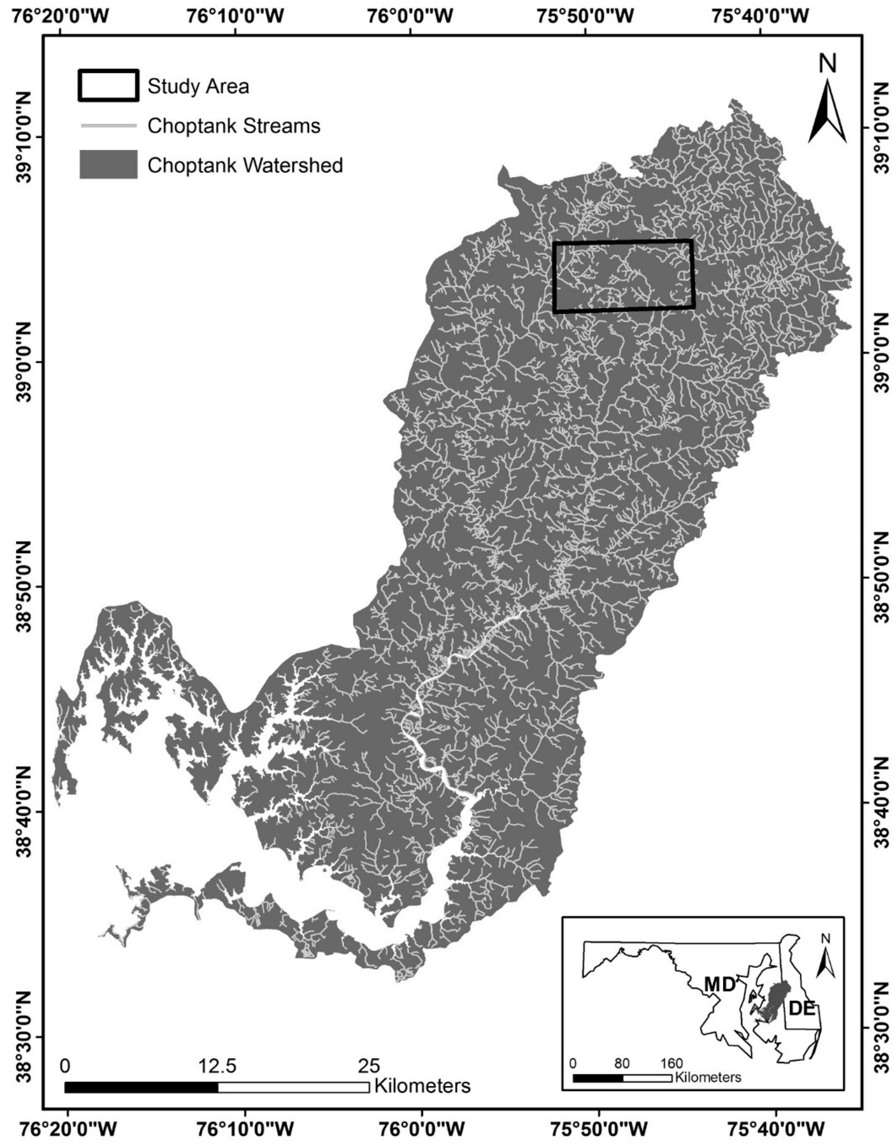
Figure 2.
A graphical representation of the normalization process, which corrects for the influence of evergreen canopy on bare earth lidar intensity data. Abbreviations used in the equations are provided earlier within the flow chart.
Figure 2.
A graphical representation of the normalization process, which corrects for the influence of evergreen canopy on bare earth lidar intensity data. Abbreviations used in the equations are provided earlier within the flow chart.
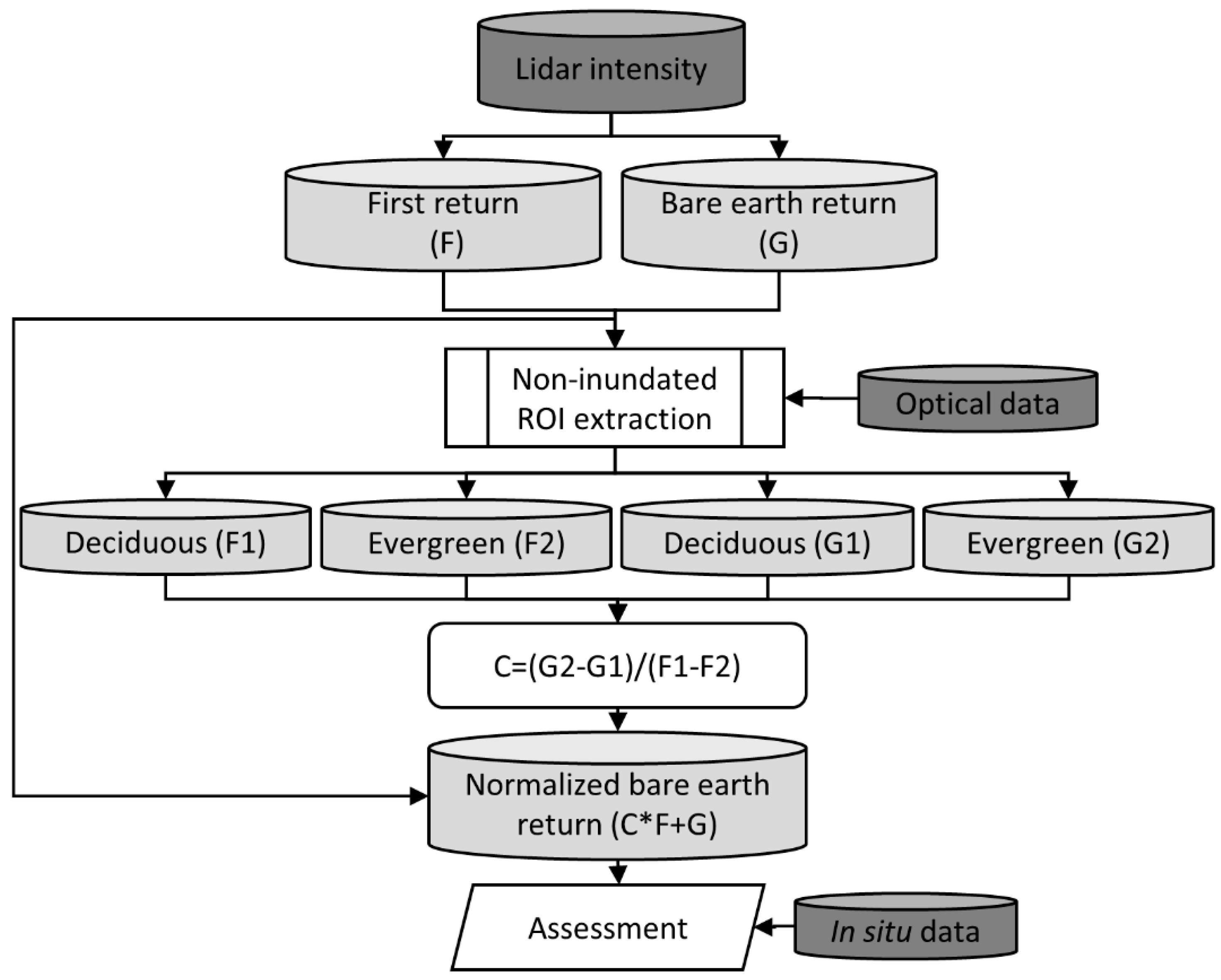
Figure 3.
Frequency distributions plotted at 5 digital number (DN) intervals depicting 27 March, 2007 (top) and 24 March, 2009 (bottom) bare earth return values extracted for in situ data points, including evergreen, inundated deciduous, and non-inundated deciduous points. All evergreen points were non-inundated.

Figure 4.
Scatterplot illustrating the median, mean, 10th, 25th, 75th, and 90th percentiles for evergreen, non-inundated deciduous and inundated deciduous region of interest (ROI) values extracted from the 27 March, 2007 (top) and 24 March, 2009 (bottom) bare earth (x-axis) and first return (y-axis) intensity images as digital numbers (DN). Note that the two deciduous classes have similar first return values, but markedly different bare earth returns, while the evergreen values are more similar to the inundated deciduous bare earth values but have markedly different first return values.
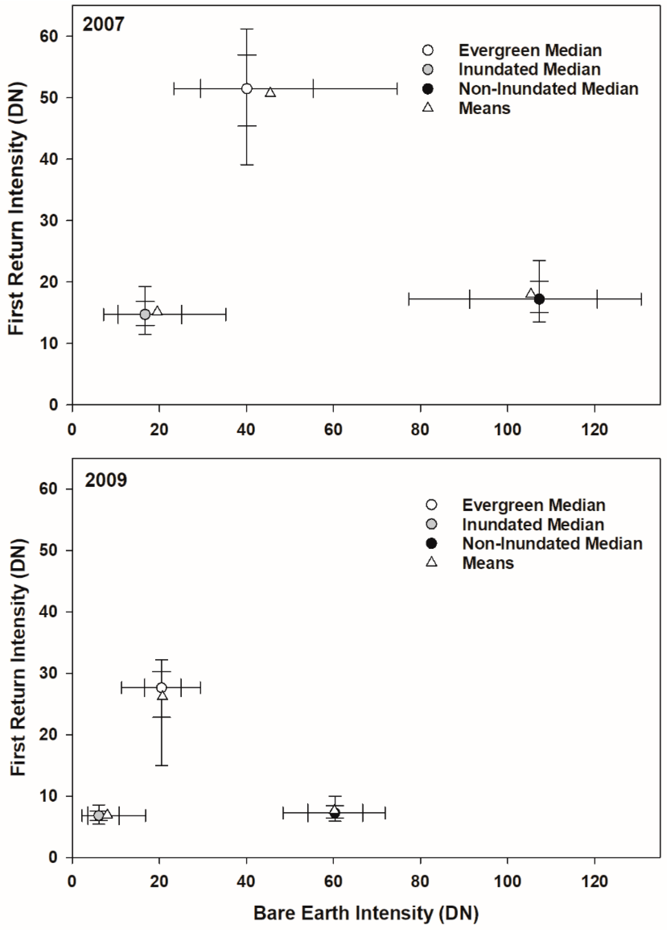
Figure 5.
Statistics for evergreen (EG), non-inundated deciduous (NID), and inundated deciduous (ID) ROIs collected from the normalized 27 March, 2007 (top) and 24 March, 2009 (bottom) bare earth intensity images as digital numbers (DN). Statistics include mean (dash line), median (solid line), 10th percentile (lower whisker), 25th percentile (lower box extent), 75th percentile (upper box extent), and 90th percentile (upper whisker). Note that after normalization the evergreen and non-inundated deciduous values are similar, while inundated deciduous values are significantly different.
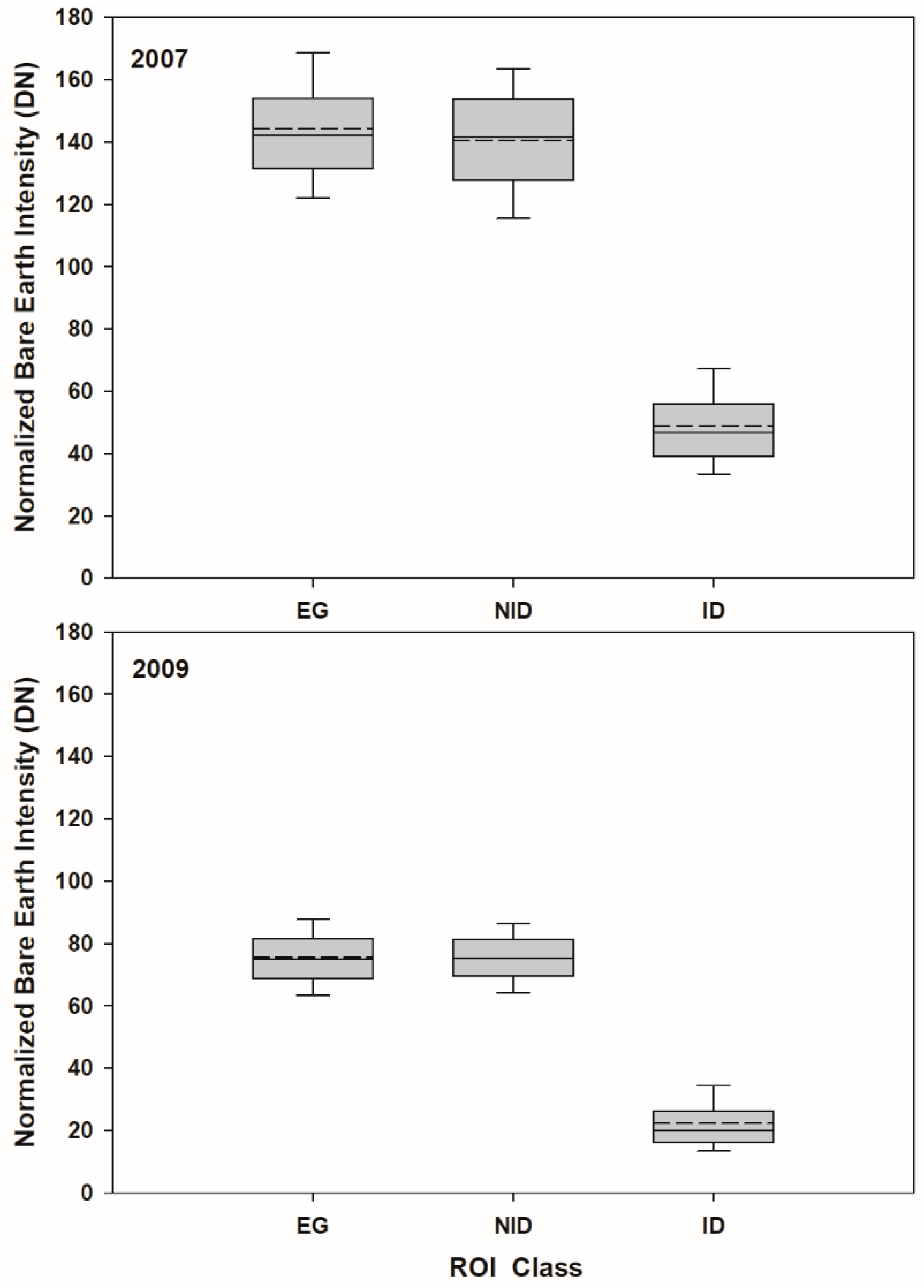
Figure 6.
Frequency distributions plotted at 5 digital number (DN) intervals depicting 27 March, 2007 (top) and 24 March, 2009 (bottom) normalized bare earth return values extracted for in situ data points, including evergreen, inundated deciduous, and non-inundated deciduous points. Note that all evergreen points were non-inundated.
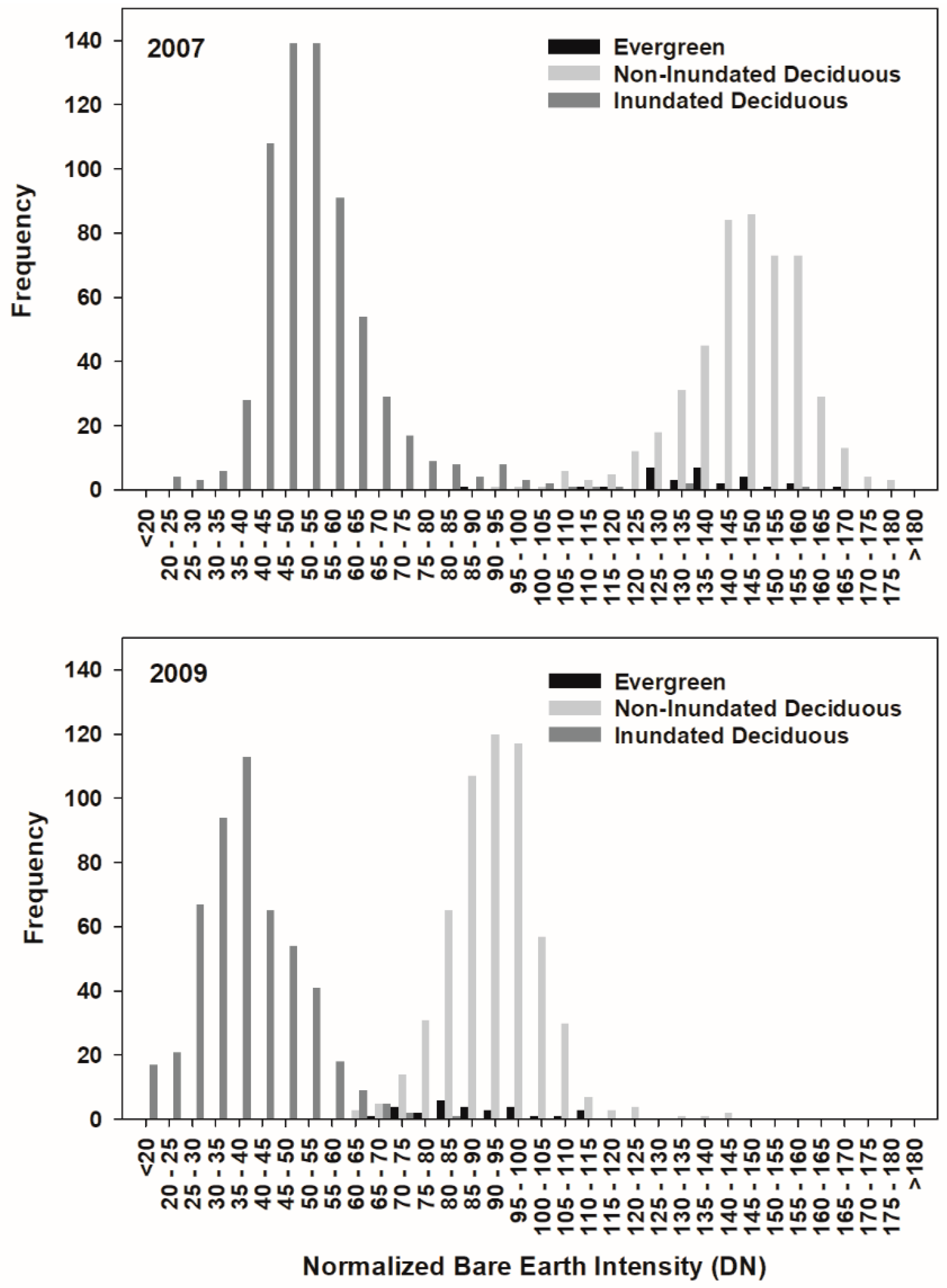
Figure 7.
Bare earth (left), first (middle), and normalized bare earth return images (right) from 27 March, 2007 (top) and 24 March, 2009 (bottom) for the same area of mixed deciduous and evergreen forest. Note that inundated areas (dark signature) are easier to identify on the normalized bare earth images relative to the original bare earth images, and that while bare earth images change between years, first return images remain relatively constant.
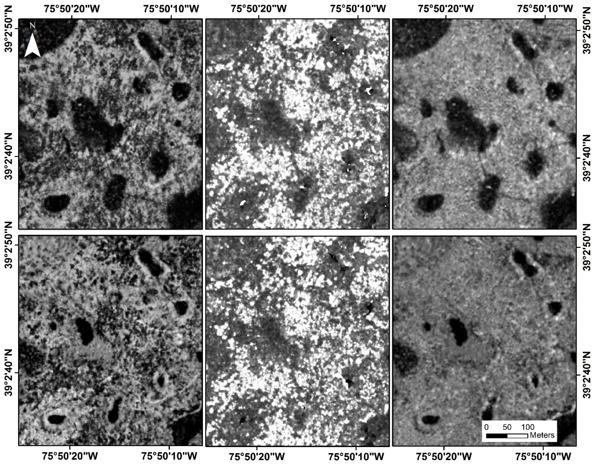
Figure 8.
Inundation map for 27 March, 2007 featuring inundated and non-inundated forest classes, as well as the transitional class. Note that the transitional class is generally found adjacent to the inundated class, but it is also found on hummocks within inundated areas, along ditches, and in other areas of low elevation.
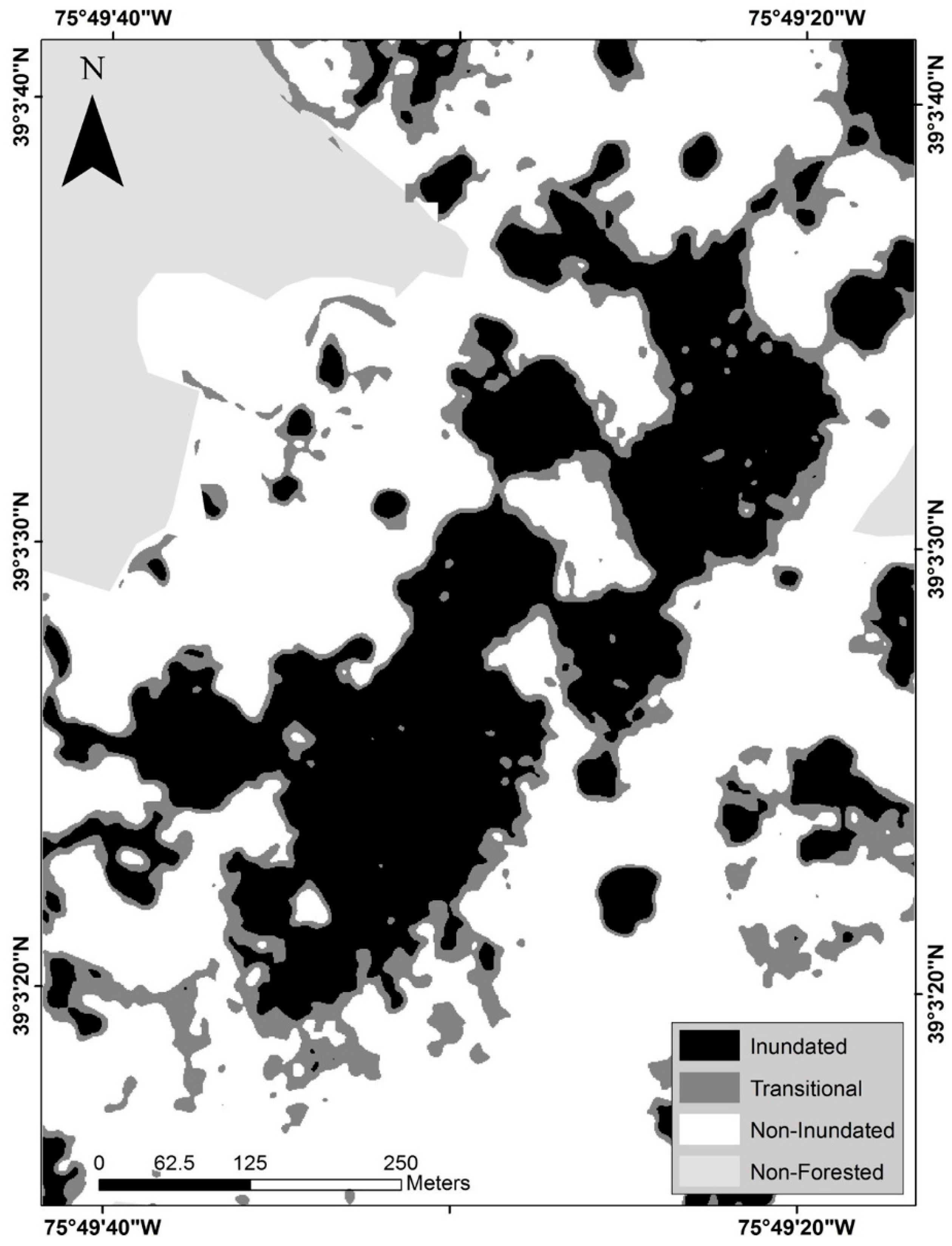
Figure 9.
Maximum likelihood classification of forested wetland inundation based on inundation training data derived from the 2007 lidar intensity data and coincident optical imagery. Panel (a) is 2007 digital false-color imagery with the red box showing the calibration extent and the blue box showing the classification extent. Panels (b,c) are the inundation training datasets derived from non-normalized and normalized bare earth 2007 lidar intensity data, respectively. Panels (d,e) are the classification results based on trained classifiers using non-normalized and normalized bare earth 2007 lidar intensity data, respectively.


Table 1.
Error matrices for 27 March, 2007 (left) and 24 March, 2009 (right). Field data indicating non-inundated (NID) and inundated (ID; top), are compared with map classes (side). Evergreen sites are indicated separately using parentheses, and were added to directly adjacent values when computing accuracy. User’s accuracy (i.e., how often the mapped class will be found in the field) is displayed vertically and producer’s accuracy (i.e., how often classes in the field are correctly classified in a map) is displayed horizontally. Overall accuracy is 99.4 % and 100.0 % for 2007 and 2009, respectively. Data for transitional field sites are indicated in gray. These numbers are included for visual reference only, and are not included in any derived estimates of accuracy.
| Year | Field Validation (2007) | Field Validation (2009) | ||||
|---|---|---|---|---|---|---|
| NID | ID | Accuracy | NID | ID | Accuracy | |
| Non-Inundated | 502(28) | 5 | 99.1% | 586(26) | 0 | 100.0% |
| Transitional | 11(1) | 15 | 10(4) | 2 | ||
| Inundated | 1(1) | 637 | 99.7% | 0 | 505 | 100.0% |
| Accuracy | 99.6% | 99.2% | 100.0% | 100.0% | ||
© 2020 by the authors. Licensee MDPI, Basel, Switzerland. This article is an open access article distributed under the terms and conditions of the Creative Commons Attribution (CC BY) license (http://creativecommons.org/licenses/by/4.0/).
Share and Cite
MDPI and ACS Style
Lang, M.W.; Kim, V.; McCarty, G.W.; Li, X.; Yeo, I.-Y.; Huang, C.; Du, L. Improved Detection of Inundation below the Forest Canopy using Normalized LiDAR Intensity Data. Remote Sens. 2020, 12, 707. https://doi.org/10.3390/rs12040707
AMA Style
Lang MW, Kim V, McCarty GW, Li X, Yeo I-Y, Huang C, Du L. Improved Detection of Inundation below the Forest Canopy using Normalized LiDAR Intensity Data. Remote Sensing. 2020; 12(4):707. https://doi.org/10.3390/rs12040707
Chicago/Turabian StyleLang, Megan W., Vincent Kim, Gregory W. McCarty, Xia Li, In-Young Yeo, Chengquan Huang, and Ling Du. 2020. "Improved Detection of Inundation below the Forest Canopy using Normalized LiDAR Intensity Data" Remote Sensing 12, no. 4: 707. https://doi.org/10.3390/rs12040707
Note that from the first issue of 2016, this journal uses article numbers instead of page numbers. See further details here.