Error Estimation of Pathfinder Version 5.3 Level-3C SST Using Extended Triple Collocation Analysis


1
Cooperative Institute for Satellite Earth System Studies (CISESS)-Maryland, University of Maryland, College Park, MD 20740, USA
2
National Centers for Environmental Information (NCEI), NOAA/NESDIS, Silver Spring, MD 20910, USA
3
Cooperative Institute for Research in Atmosphere (CIRA), Colorado State University, Fort Collins, CO 80523, USA
4
Center for Satellite Applications and Research (STAR), NOAA/NESDIS, College Park, MD 20740, USA
5
National Centers for Environmental Information (NCEI), NOAA/NESDIS, Asheville, NC 28801, USA
*
Author to whom correspondence should be addressed.
Remote Sens. 2020, 12(4), 590; https://doi.org/10.3390/rs12040590
Submission received: 27 January 2020
/
Revised: 6 February 2020
/
Accepted: 8 February 2020
/
Published: 11 February 2020
(This article belongs to the Special Issue Advances in Retrieval, Operationalization, Monitoring and Application of Sea Surface Temperature)
Abstract
:Sea Surface Temperature (SST) is an essential climate variable (ECV) for monitoring the state and detecting changes in the climate. The concept of ECVs, developed by the Global Climate Observing System (GCOS) program of the World Meteorological Organization (WMO), has been broadly adopted in worldwide science and policy circles Besides being a climate change indicator, the global SST field is an essential input for atmospheric models, air-sea exchange studies, understanding marine ecosystems, operational weather, and ocean forecasting, military and defense operations, tourism, and fisheries research. It is, therefore, critical to understand the errors associated with SST measurements from both in situ measurements and satellite observations. The customary way of validating a satellite SST is to compare it with in situ measured SSTs. This method, however, will have inaccuracies due to uncertainties involving both types of measurements. A triple collocation (TC) error analysis can be implemented on three mutually independent error-prone measurements to estimate the root-mean-square error (RMSE) of each measurement. In this study, the error characterization for the Pathfinder SST version 5.3 (PF53) dataset is performed using an extended TC (ETC) method and reported to be in the range of 0.31 to 0.37 K. These values are reasonable, as is evident from corresponding very high (~0.98) unbiased signal-to-noise ratio (SNR) values.
1. Introduction
Sea Surface Temperature (SST) is an essential climate variable used to monitor, detect, predict and characterize earth’s climate and its variations [1]. Several long-term global SST records are available, based on observations acquired from sailing vessels in earlier decades and, in more modern times, from in situ measurements (from drifters, moored buoys, Argo floats, etc.) and from space and airborne sensors (on satellites and aircraft) [2,3]. The advantage of satellite-derived SSTs compared to other sources is vast coverage at high resolution. However, they also have inherent inaccuracies due to the errors associated with spacecraft navigation, sensor calibration and noise, retrieval algorithms, and residual clouds. As a result, there is a need to provide clear error estimates associated with satellite SSTs in order to obtain the desired results in their intended applications. Validation and cross-comparison of different satellite-derived SSTs are critical to understanding these products and to assess their relative merit and performance. However, differences of several degrees can appear between various products due to inconsistencies in retrieval schemes and in cloud detection algorithms [4]. Therefore, confidence in the reported accuracy of any retrieval is dependent on the validation procedure.
For validation purposes, most satellite-based SSTs are compared against collocated in situ measurements, which, although considered as ‘true’ values for comparison purposes, also have errors associated with them. The reported inaccuracies partly originate from the spatiotemporal mismatch between the in situ and satellite locations, and the standard deviation in their differences has contributions from both of them. Thus, through direct comparison, it is not possible to decouple estimated error associated with the satellite-derived SSTs only. A real validation of any geophysical target variable requires an accurate characterization of the associated errors. A direct comparison of satellite-derived SST with in situ data does not yield the real error in the satellite SST, as there will be ambiguity due to errors both of them and of collocation differences. The situation is further complicated by the fact that buoy data are not uniformly distributed in space and time over the global oceans and have varying performances owing to different origins (cf. [5]), as well as that the quality of the in situ drifter measurements cannot easily be verified once a drifter has been deployed at sea (cf. [6]). Also, these measurements are collected at depths ranging from 0.1 m to 2 m below the sea surface and, therefore, may not be fully consistent with satellite infrared SST measurements, which are representative only at depths of approximately the channel wavelength (mostly near-surface, in the micrometer to millimeter range).
Direct validation of SSTs from satellite infrared radiometry is allowed by coincident ship-borne skin measurements made below the intervening atmosphere (cf. [7,8,9,10]). However, the availability of such data has long been recognized to be sparse e.g., [11,12,13,14] and still continues to be rather limited [6]. In addition to algorithmic and reference-related differences between retrieved SSTs, some differences are due to practicalities and lack of a consensus in validation approaches. These include (a) different criteria for matchup between the product and the reference, (b) different treatment of outliers in retrievals, references, or both, (c) using hard cutoffs to exclude tail-end elements from the matchup probability density function, (d) averaging satellite retrievals that may smooth the noise, and (e) reporting only robust statistics. While no particular approach can be proclaimed as the ‘best practice’, since all are driven by the purpose of validation (cf. [15]), the situation creates difficulties in the assessment of product performance from a user perspective because of the lack of a common platform. These challenges have been recognized by the Group for High-Resolution Sea Surface Temperature (GHRSST), leading to the formation of the Satellite Sea-Surface Temperature Working Group (ST-VAL) (https://www.ghrsst.org/about-ghrsst/tags-and-wgs/), with an objective of facilitating best practices for validation in the international SST community.
Validation against in situ data is performed primarily for the purposes of assessing the accuracy (bias) and precision (standard deviation) of the target products. Also, most products are generated by regression techniques, against in situ data or based on radiative transfer simulations, and may empirically be tied to the ‘reference response variable’, e.g., drifters. To investigate the independence of the various products, the correlations between the residuals should also be analyzed. Additionally, in situ, data are expected to have inherent measurement error, as with any physical system, which will affect the validation statistics. This inherent limitation can be overcome by employing a triple collocation method (TCM) on triplets of collocated matchups.
A triple collocation (TC) three-way error analysis of three mutually independent measurements can be used to estimate the root-mean-square error (RMSE) of each of these measurements with a high level of accuracy. As mentioned earlier, a knowledge of the ‘true’ value of SST is desirable to estimate the error with high accuracy, but the ‘true’ observations are themselves imperfect due to inherent errors. Using a TC error analysis, it is possible to estimate the RMSE without treating any one system as perfectly observed ‘truth’ [16], thus estimating only the random error associated with the target variable. TC has also been used widely in oceanography for SST error estimation [17,18,19], wind speed, and wind stress [20,21] and wave height [22,23]. This standard TC approach provides RMSE of the measurement system, which represents the variability of the measurement error.
In this study, the concept of TC is extended to estimate the correlation coefficient of each measurement system with respect to the unknown target variables of SST, based on the work of McColl et al. [24]. Thus, we are estimating not only the errors associated with our target variable but also the sensitivity of the measurement system to the ‘true’ SST. In this extended triple collocation (ETC) analysis, the estimation of the correlation coefficient is obtained without using any additional assumptions other than what is already used in TC analysis. Using ETC, we determine the RMSEs and unbiased signal-to-noise ratios (obtained from the correlation coefficients) for the Pathfinder Version 5.3 Level-3C SST product (PF53) using 14 years (1998–2011) of Climate Data Record, along with the in situ SST data and the Advanced Along Track Scanning Radiometer (AATSR) Reprocessing of Climate (ARC) dataset for the corresponding period. These three SST observations are collocated, and statistics of the difference between each pair are estimated. The variances of these differences are further used to derive the RMSE related to each observation type independently (assuming uncorrelated errors). The next section provides a brief review of TC along with an overview of the ETC for this analysis. The implementation of ETC and the results are discussed in the final sections.
2. Methodology
2.1. Triple Collocation Theory
To determine the errors associated with a measurement system for a geophysical variable, the TC method uses a linear error model (Equation (1)) [25].
where ‘Xi’ (with i = 1,2,3) are collocated measurement systems linearly related to the true value of ‘t’ with as additive random errors, and as the ordinary least-square (LS) intercept and slope, respectively. Apart from the assumption of the linear error model, the TC approach makes two further assumptions, that all the errors are mutually uncorrelated and are also uncorrelated with the truth (unknown target variable). It is also required for the errors of each independent source to have ‘zero’ mean. The covariance between these different measurement systems [24] can be stated as:
Assuming that the errors from independent sources have zero mean and are uncorrelated with each other and with true value t . With as the variance of and the assumptions above, the two middle terms on the right-hand side are zero, and so is the last term when . Equation (2), thus reduces to:
The TC analysis further involves a two-step process: a reference dataset is picked arbitrarily, followed by an optimal rescaling of the remaining dataset to remove any biases due to [26], leading to a simplified equation for RMSE estimates. However, in this study, we follow McColl et al. [24] instead of rescaling. Using six unique terms of a 3 × 3 covariance matrix (Q11, Q12, Q13, Q22, Q23, Q33), and defining a new variable ; Equation (3) can be solved to obtain the TC estimation equation for RMSE as:
2.2. Extended Triple Collocation
In the ETC technique, the obtained from TC is used to solve the correlation coefficient of the measurement system with respect to the unknown truth. McColl et al. [24] use an ordinary least square solution for Equation (1) in the form of:
where is the correlation coefficient between t and Xi, t is the true value of the variable, with the assumption that it has no measurement error; Xi, is the measurement variable. Using the relation between and , and a solution obtained for from Equation (3), the correlation coefficient can be estimated in terms of covariance values as:
Thus, ETC provides the correlation coefficient with a sign ambiguity; however, in practice, the value is always positive. The significance of the correlation coefficient is evident by modifying Equation (5) and obtaining:
where (or ) is the unbiased signal-to-noise ratio varying from 0 to 1. The square of the correlation coefficient, also known as the unbiased SNR, will have a combined effect of the sensitivity of the measurement system (), the variability of the true signal (), and the variability of the measurement error (), whereas the TC only provided the information on . This correlation coefficient has been widely used in many previous validation studies e.g., [27,28,29].
3. Dataset
3.1. Pathfinder Data
Pathfinder Version 5.3 (PF53) Level-3 Collated (L3C) Sea Surface Temperature (SST) is a retrospectively processed skin-level SST dataset available from 1981 to present for climatological applications [30]. This dataset, representing ~37 years of global, twice-daily (day/night) 4 km SST data, is produced by the NOAA National Centers for Environmental Information (NCEI) and is generated with measurements combined from a single AVHRR instrument (at a time) into a space-time grid. Thus, one time of dataset is a combination of multiple passes/scenes combined together. A long-term data record of SST, such as Pathfinder is highly desirable for various applications like atmospheric and ocean modelling, coral-reef bleaching, understanding the variability of fisheries yields, and analysis of extreme climate events [31,32,33,34]. For this analysis, Pathfinder version 5.3 L3C data is obtained on a daily basis from 1998 to 2011 by pulling it from the ftp site (https://doi.org/10.7289/v52j68xx). The PF53 dataset is in the GHRSST Data Specification version 2 (GDS2) format and has a quality level flagged for every pixel that provides an indicator for the overall quality of an SST measurement. The quality flags vary from 0 to 5, with 0 used to indicate missing data, 1 as invalid data, and 2–5 as the worst to the best quality of usable data, respectively. For this analysis, we used the highest values of GHRSST quality flag (qf = 5), considered to be the best quality available.
3.2. Buoy Data
The in situ data are obtained from the iQuam2 repository [35], which contains in situ SST data from 1981 to the present from various sources. Ship and buoy (drifters and moorings) data come from the International Comprehensive Ocean-Atmosphere Data Set (ICOADS) (Sep 1981–Nov 2007) and Global Telecommunications System (GTS) (Dec 2007–present) data. Real-time NCEP GTS are refreshed every 12 h and are ingested into iQuam2 routinely. ARGO data on US GODAE/GDAC (https://www.seanoe.org/data/00311/42182/) are refreshed and ingested in a delayed mode. ICOADS and ARGO data come with their own quality flags (QFs) and quality indicators (QI), which are preserved in iQuam2 output files. ICOADS QFs are not used in iQuam2 Quality Control (QC). Also, OSI SAF ‘blacklist’ QF is reported in the iQuam2 output files but not used in the iQuam2 QC. On the other hand, ARGO QFs are used to select the best quality near-surface data from 3–7 m depth, which are further subject to the standard iQuam QC. These datasets are, thus quality controlled using the GHRSST quality flag system, and the bad buoys are normally flagged out. The data are downloaded from iQuam’s ftp site (ftp://ftp.star.nesdis.noaa.gov/pub/socd/sst/iquam/v2.00/), and only the best quality data (QF = 5) is used in this analysis. While in situ data has its own limitations (cf. [36], which lists related references), it is still considered as the gold standard for validation. A quality-controlled in situ dataset (such as iQuam2) with unphysical values removed is needed for a ‘true validation’.
3.3. ARC Data
The third independent dataset used for this study is the Level-3 (L3) SST from AATSR Reprocessing for Climate (ARC). The ARC dataset consists of Advanced Along-Track Scanning Radiometer (AATSR) multimission data, which has been reprocessed using various algorithms and in situ contemporaneous measurements to provide update retrievals of SST and assess their accuracy. The ATSR instruments are dual-view radiometers with one aperture directed towards nadir and the other at a view angle of 55° to zenith [37]. Embury and Merchant [38] details out the retrieval scheme for ARC data and has SST retrievals available in different modes, e.g., in separate ‘nadir’ view and ‘dual’ (nadir + slant) view, as well as two other modes in terms of a two-window (10.8 and 12 μm) channel or three-window (3.7, 10.8, and 12 μm) channel retrieval. As three-window channel retrieval is valid only for the night due to solar contamination in daylight hours, we use the dual-window channel retrievals of nighttime and daytime data for the sake of consistency along with nadir-only data. In this study, ARC data from 1998 to 2011, available as Version 1.1.1, is obtained from the Natural Environment Research Council (NERC) Center for Environmental Data Analysis (CEDA) repository [39]. This version of ARC data is the latest and uses a cloud mask based on a probabilistic Bayesian method discussed in Merchant et al. [40]. The ARC data are daily files with SST as one of the variables on a 0.1° × 0.1° grid.
3.4. Matchup Data
Note that all three datasets are concurrently obtained for the 14-year period (1998–2011), as this was the only long time period for which we have collocated measurements of Level-3 SST data. Both the Pathfinder and ARC based L3C SSTs are available twice a day, with one file each corresponding to day and night. For this study, a separate matchup database for daytime and nighttime was developed. The time for in situ measurements is derived based on the solar zenith angle information associated with each observation in the iQuam files, which is further used to divide the data into day or night broadly. The nearest neighborhood method is used to match all in situ data inside a satellite grid. Thus, both daytime and nighttime matchups are developed. A triple matchup for each is further developed from these daytime and nighttime matchups.
4. Results
4.1. Validation with in Situ
The PF53 SSTs were previously validated against SSTs from drifting buoys [Climate Data Record (CDR) Climate-Algorithm Theoretical Basis Document (C-ATBD)]. The comparison statistics in nighttime matchups, including median bias (accuracy) and robust standard deviation (precision) for 14 years (1998–2011), are reproduced here in Table 1 (readers may refer to the tables 5A to 12B in the CDR report for statistics from other years). Note that only the best quality iQuam2, as well as the PF53 data, are used for this analysis.
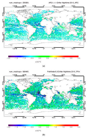
The ARC data from 1998 to 2011 are also matched up with iQuam2 data. These matchup databases (MDB) are generated for each year, depending on the number of good-quality in situ data available. For example, Figure 1a,b shows a full-year matchup of ARC with drifting buoys (a) and Pathfinder (b). These matchups are in the range of ~0.3 to 0.5 million for the years 2010 and 2011 but drastically reduced for the years prior to 2008 (last two columns in Table 1).
These results show that there is a cold bias for PF53 data in the range of ~ −0.17 to −0.31 K, and a standard deviation of ~0.39 to 0.49 K. ARC also shows a cold bias of ~ −0.15 to −0.23 K and a standard deviation in the range ~0.31 to 0.36 K. The negative mean bias for both PF53 and ARC is primarily attributed to the ‘cool-skin’ effect (which may account for a cold bias of about −0.17 K on average [8], (CDR C-ATBD document 2016), but some effect of residual cloud cannot be ruled out. Ideally, skin products should be validated against ‘skin’ reference SSTs, such as radiometer measurements (cf. [41]), but this is beyond the objective and the scope of this study.
4.2. Assumption of Data Independence
Ideally, the three SST products used in this study should be maximally independent of each other. In reality, correlations between products are observed to different degrees, induced by a combination of contributions from the sensor, algorithm, and the cloud-mask. For any given SST product pair, if they are correlated, ordered values of one data will occur consistently with the same of the other product. Conversely, there will be no specific pattern if the data are fully independent of each other. This is checked using bivariate density (joint probability) plots in residual space (SST minus in situ measurements (here, drifters), as shown in Figure 2. The matchups are for data between January 1998 and November 2011. The night and day time bivariate density plots clearly show a low correlation (R2) value of ~0.25−0.33 in the residuals, as both products are developed from different sensors (AVHRR for PF53 and AATSR for ARC) and have a low or minimal contribution from drifters. This supports the assumption that both the errors in these products are independent of each other. Thus, going back to one of the assumptions for the ETC, it is acceptable to say that both the products used here are independent and that the ETC method can be used to determine the true variability of each target SSTs. The R2 values using other in situ data are ~0.66 (with ships), ~0.33 (TM buoys), ~0.35 (CM buoys), and 0.21 (Argo).
4.3. Triple Collocation
In an attempt to understand the true noise associated with different products, we have employed the extended triple collocation method to perform a three-way error analysis. The matchup databases developed here are used to create appropriate triplets, as described in Section 2. These matchup numbers decrease to tens of thousands to thousands when the triple collocation is applied to compare the ARC and PF53 data. For all these statistics, only the best quality (QF = 5) PF53 data is used. Figure 3a–e shows RMSEs of ARC, PF53, and in situ data derived from the triple collocation between the three datasets for nighttime only. For each combination, in situ data (drifters, ship, tropical moorings, coastal moorings, and Argo floats) is the transfer comparison standard (reference). With drifters as in situ transfer standards, the RMSE ranges from 0.29 to 0.37 K for PF53, 0.25 to 0.32 K for drifters, and 0.19 to 0.25 K for ARC data. In the case of ship data, the RMSE values of PF53 and ARC are closer to each other (~0.30 to 0.44 K). For Tropical Mooring and Coastal Moorings as transfer standards, ARC data RMSE varies between 0.2 to 0.4 K, while for PF53, the RMSEs are a bit higher (~0.25 to 0.45 K).
In the case of ARGO floats as transfer standards, RMSE for ARC is in the range 0.1 to 0.35 K; for PF53, it is 0.15 to 0.4 K, while it is in the range 0.1 to 0.4 K for ARGO. Figure 3f provides the time series of the number of triple collocated matchups for each standard transfer, with a high exponential increase in the case of drifting buoys, followed by coastal mooring, tropical mooring, and the rest. For drifters, the number of matchups is between a few thousand to 40,000 a year. For TM, it is in the order of a few thousand, and for ARGOs, it is in the hundreds. A slightly lower value of RMSE for ARC as compared to PFSST does not necessarily imply that it’s a better product, as the spatial distribution of pixels in the case of ARC data is much less and will limit some practical applications. Table 2 shows the nighttime RMSEs for PF53 SST and ARC SST and the in situ data using the ETC three-way error analysis using 14 years of statistics. The RMSE values are more or less the same for the daytime matchups, with slight differences as provided in the corresponding parenthesis.
The time series of PF53 and ARC RMSEs are consistent irrespective of the insitu anchor data, and both datasets are also stable with time. As compared to the results from Xu and Alexander [19], most of their AVHRR RMSEs either match or have slightly higher values w.r.t. PF53 RMSEs. Thus, inferring that the random errors in AVHRR based PF53 are comparable or slightly better than the other reported values [19]. However, the RMSEs of drifters and T-moorings are slightly higher than the other published analyses [17,18,19]. As expected, the Argo RMSEs at night are similar to the corresponding nighttime drifter RMSEs although there is a difference in their observation depths.
Figure 4 shows the unbiased signal-to-noise ratio or SNRUB for each dataset with different in situ data transfer standards. These in situ data standards range from drifters, ship, tropical moorings, and coastal moorings to Argo floats (Figure 4a–e). It can be inferred that the unbiased SNR values range from 0.95 to 0.99, which is very high. These high SNR values ensure that the RMSE estimates provided in Figure 3 are reasonable and realistic. That is, a given RMSE value can be too high if the is low (low sensitivity), but the same RMSE will be acceptable if the is very high (high sensitivity). For all three datasets (in situ, ARC, and PF53), the higher value of the correlation coefficient corresponds to the lower value (or dip) in RMSE.
5. Conclusions
Validation results of satellite-derived SST products against in situ SSTs have inherent inaccuracies resulting from spatiotemporal inhomogeneity between the satellite and the point measurements. In addition, such validation requires treating the reference data (in this case in situ SSTs) as the ‘true’ value of SST, in the process neglecting the error in the in situ data. A triple collocation based three-way error analysis using three mutually independent error-prone measurements can be used to calculate RMSEs associated with each of the measurements without treating any one of them as the ‘truth’. In this study, we estimated the RMSEs associated with the Pathfinder Version 5.3 Level-3C SST product. The other two data sources used for this analysis are the iQuam2 in situ SSTs and the AATSR-based ARC dataset for the corresponding period. Firstly, a triple matchup of the dataset was created, and subsequently, the RMSEs and corresponding unbiased SNRs for each data source was estimated by employing the Extended Triple Collocation (ETC) method. The RMSE (true variability) ranged from 0.31 to 0.37 K for PF53, and 0.18 to 0.33 K for the ARC data. These values were reasonable, as was evident from the very high unbiased SNR values (~0.98). The ETC method used to estimate the random error for the Pathfinder SST had some inherent limitations (weaknesses). The results are heavily dependent on our three main assumptions, (1) the error model, (2) independent errors between in situ data, PF53, and ARC and (3) independence of the error from true value of the variable. If any of these assumptions failed, it could lead towards inaccurate values of RMSEs. However, ETC is a powerful technique and is easy to implement. In the future, as an extension of this study, we will work towards the spatial distribution of the error associated with the Pathfinder SST.
Author Contributions
Conceptualization: K.S. and P.D.; Methodology: K.S. and P.D.; Software: K.S.; Validation: K.S.; Formal Analysis: K.S.; Investigation: K.S., P.D., X.Z., H.-m.Z.; Resources: K.S., P.D., X.Z., H.-m.Z.; Data Curation: K.S.; Writing-Original Draft Preparation, K.S.; Writing-Review & Editing, K.S., P.D., X.Z., H.-m.Z.; Visualization, K.S., P.D.; Supervision, K.S.; Project Administration, H.-m.Z. and X.Z. All authors have read and agreed to the published version of the manuscript.
Funding
This research received no external funding.
Acknowledgments
We thank the NOAA NCEI Articles Review Process for reviewing the manuscript and helping us with technical editing. Thanks to our NOAA colleague Tim Boyer for making the internal review process smooth. We are very thankful to the reviewers for their detailed review of our manuscript. The views, opinions, and findings contained in this paper are those of the authors and should not be construed as an official NOAA or US Government position, policy, or decision.
Conflicts of Interest
The authors declare no conflict of interest.
References
- Bojinski, S.; Verstraete, M.; Peterson, T.C.; Richter, C.; Simmons, A.; Zemp, M. The Concept of Essential Climate Variables in Support of Climate Research, Applications, and Policy. Bull. Am. Meteorol. Soc. 2014, 95, 1431–1443. [Google Scholar] [CrossRef]
- Hagan, D.; Rogers, D.; Friehe, C.; Weller, R.; Walsh, E. Aircraft observations of sea surface temperature variability in the tropical Pacific. J. Geophys. Res. 1997, 102, 15733–15747. [Google Scholar] [CrossRef]
- Donlon, C.; Robinson, I.; Casey, K.S.; Vazquez-Cuervo, J.; Armstrong, E.; Arino, O.; Gentemann, C.; May, D.; LeBorgne, P.; Piollé, J.; et al. The Global Ocean Data Assimilation Experiment High-resolution Sea Surface Temperature Pilot Project. Bull. Am. Meteorol. Soc. 2007, 88, 1197–1214. [Google Scholar] [CrossRef]
- Merchant, C.J. Thermal Remote Sensing of Sea Surface Temperature. In Thermal Infrared Remote Sensing, Remote Sensing and Digital Image Processing; Kuenzer, C., Dech, S., Eds.; Springer: Dordrecht, The Netherlands, 2013; Volume 17. [Google Scholar]
- Garraffo, Z.D.; Mariano, A.J.; Griffa, A.; Veneziani, C.; Chassignet, E.P. Lagrangian data in a high-resolution numerical simulation of the North Atlantic I. Comparison with in situ drifter data. J. Mar. Syst. 2001, 29, 157–176. [Google Scholar] [CrossRef]
- Donlon, C.J.; Wimmer, W.; Robinson, I.; Fisher, G.; Ferlet, M.; Nightingale, T.; Bras, B. A second-generation blackbody system for the calibration and verification of seagoing infrared radiometers. J. Atmos. Ocean. Technol. 2014, 31, 1104–1127. [Google Scholar] [CrossRef]
- Suarez, M.J.; Emery, W.J.; Wick, G.A. The multi-channel infrared sea truth radiometric calibrator (MISTRC). J. Atmos. Ocean. Technol. 1997, 14, 243–252. [Google Scholar] [CrossRef]
- Kearns, E.J.; Hanafin, J.A.; Evans, R.H.; Minnett, P.J.; Brown, O.B. An Independent Assessment of Pathfinder AVHRR Sea Surface Temperature Accuracy Using the Marine Atmosphere Emitted Radiance Interferometer (MAERI). Bull. Am. Meteorol. Soc. 2000, 81, 1525–1536. [Google Scholar] [CrossRef] [Green Version]
- Noyes, E.J.; Minnett, P.J.; Remedios, J.J.; Corlett, G.K.; Good, S.A.; Llewellyn-Jones, D.T. The accuracy of the AATSR sea surface temperatures in the Caribbean. Remote Sens. Environ. 2006, 101, 38–51. [Google Scholar] [CrossRef]
- Minnett, P.J.; Corlett, G.K. A pathway to generating climate data records of sea-surface temperature from satellite measurements. Deep Sea Res 2012, 77–80, 44–51. [Google Scholar] [CrossRef]
- Donlon, C.J.; Keogh, S.J.; Baldwin, D.J.; Robinson, I.S.; Ridley, I.; Sheasby, T.; Barton, I.J.; Bradley, E.F.; Nightingale, T.J.; Emery, W. Solid-state radiometer measurements of sea surface skin temperature. J. Atmos. Ocean. Technol. 1998, 15, 775–787. [Google Scholar] [CrossRef]
- Minnett, P.J.; Knuteson, R.O.; Best, F.A.; Osborne, B.J.; Hanafin, J.A.; Brown, O.B. The Marine-Atmospheric Emitted Radiance Interferometer: A high-accuracy, seagoing infrared spectroradiometer. J. Atmos. Ocean. Technol. 2001, 18, 994–1013. [Google Scholar] [CrossRef]
- Jessup, A.T.; Branch, R. Integrated ocean skin and bulk temperature measurements using the calibrated infrared in situ measurement system (CIRIMS) and through hull-ports. J. Atmos. Ocean. Technol. 2008, 25, 579–597. [Google Scholar] [CrossRef]
- Castro, S.L.; Wick, G.A.; Minnett, P.J.; Jessup, A.T.; Emery, W.J. The impact of measurement uncertainty and spatial variability on the accuracy of skin and subsurface regression-based sea surface temperature algorithms. Remote Sens. Environ. 2010, 114, 2666–2678. [Google Scholar] [CrossRef]
- Embury, O.; Merchant, C.J.; Corlett, G. A reprocessing for climate of sea surface temperature from the along-track scanning radiometers: Initial validation, accounting for skin and diurnal variability effects. Remote Sens. Environ. 2012, 116, 62–78. [Google Scholar] [CrossRef] [Green Version]
- Stoffelen, A. Toward the true near-surface wind speed: Error modeling and calibration using triple collocation. J. Geophys. Res. 1998, 103, 7755–7766. [Google Scholar] [CrossRef]
- O’Carroll, A.G.; Eyre, J.R.; Saunders, R.W. Three-Way Error Analysis between AATSR, AMSR-E, and In Situ Sea Surface Temperature Observations. J. Atmos. Ocean. Technol. 2008, 25, 1197–1207. [Google Scholar] [CrossRef] [Green Version]
- Gentemann, C.L. Three way validation of MODIS and AMSR-E sea surface temperatures. J. Geophys. Res. Oceans 2014, 119, 2583–2598. [Google Scholar] [CrossRef]
- Xu, F.; Ignatov, A. Error characterization in iQuam SSTs using triple collocations with satellite measurements. Geophys. Res. Lett. 2016, 43, 10826–10834. [Google Scholar] [CrossRef]
- Portabella, M.; Stoffelen, A. On scatterometer ocean stress. J. Atmos. Ocean. Tech. 2009, 26, 368–382. [Google Scholar] [CrossRef] [Green Version]
- Vogelzang, J.; Stoffelen, A.; Verhoef, A.; Figa-Saldaña, J. On the quality of high-resolution scatterometer winds. J. Geophys. Res. 2011, 116, C10033. [Google Scholar] [CrossRef] [Green Version]
- Caires, S.; Sterl, A. Validation of ocean wind and wave data using triple collocation. J. Geophys. Res. 2003, 108, 3098. [Google Scholar] [CrossRef]
- Janssen, P.A.E.M.; Abdalla, S.; Hersbach, H.; Bidlot, J.-R. Error estimation of buoy, satellite, and model wave height data. J. Atmos. Ocean. Technol. 2007, 24, 1665–1677. [Google Scholar] [CrossRef] [Green Version]
- McColl, K.A.; Vogelzang, J.; Konings, A.G.; Entekhabi, D.; Piles, M.; Stoffelen, A. Extended triple collocation: Estimating errors and correlation coefficients with respect to an unknown target. Geophys. Res. Lett. 2014, 41, 6229–6236. [Google Scholar] [CrossRef] [Green Version]
- Zwieback, S.; Scipal, K.; Dorigo, W.; Wagner, W. Structural and statistical properties of the collocation technique for error characterization. Nonlin. Process. Geophys. 2012, 19, 69–80. [Google Scholar] [CrossRef]
- Yilmaz, M.T.; Crow, W.T. Evaluation of Assumptions in Soil Moisture Triple Collocation Analysis. J. Hydrometeor. 2014, 15, 1293–1302. [Google Scholar] [CrossRef]
- Jackson, T.J.; Bindlish, R.; Cosh, M.H.; Zhao, T.; Starks, P.J.; Bosch, D.D.; Seyfried, M.; Moran, M.S.; Goodrich, D.C.; Kerr, Y.H.; et al. Validation of Soil Moisture and Ocean Salinity (SMOS) soil moisture over watershed networks in the U.S. IEEE Trans. Geosci. Remote Sens. 2012, 50, 1530–1543. [Google Scholar] [CrossRef] [Green Version]
- Mo, T.; Choudhury, B.J.; Schmugge, T.J.; Wang, J.R.; Jackson, T.J. A model for microwave emission from vegetation-covered fields. J. Geophys. Res. 1982, 87, 11229–11237. [Google Scholar] [CrossRef]
- Owe, M.; van de Griend, A.A.; Chang, A.T.C. Surface moisture and satellite microwave observations in semiarid southern Africa. Water Resour. Res. 1992, 28, 829–839. [Google Scholar] [CrossRef]
- Saha, K.; Zhao, X.; Zhang, H.; Casey, K.S.; Zhang, D.; Baker-Yeboah, S.; Kilpatrick, K.A.; Evans, R.H.; Ryan, T.; Relph, J.M. AVHRR Pathfinder Version 5.3 Level 3 Collated (L3C) Global 4 km Sea Surface Temperature for 1981-Present; Dataset; NOAA National Centers for Environmental Information: Asheville, NC, USA, 2018. [CrossRef]
- Seidov, D.; Mishonov, A.; Regan, J.; Baranova, O.; Cross, S.; Parsons, R. Regional Climatology of the Northwest Atlantic Ocean: High-Resoution Mapping of Ocean Structure and Change. Bull. Am. Meteorol. Soc. 2018, 99, 2129–2138. [Google Scholar] [CrossRef]
- Saha, K.; Zhao, X.; Zhang, H.; Casey, K.S.; Zhang, D.; Zhang, Y.; Baker-Yeboah, S.; Relph, J.M.; Krishnan, A.; Ryan, T. The Coral Reef Temperature Anomaly Database (CoRTAD) Version 6—Global, 4 km Sea Surface Temperature and Related Thermal Stress Metrics for 1982 to 2018; Dataset; NOAA National Centers for Environmental Information: Asheville, NC, USA, 2018. [CrossRef]
- Sully, S.; Burkepile, D.E.; Donovan, M.K.; Hodgson, G.; van Woesik, R. A global analysis of coral bleaching over the past two decades. Nat. Commun. 2019, 10, 1264. [Google Scholar] [CrossRef] [Green Version]
- Pinto, C.; Travers-Trolet, M.; Macdonald, J.I.; Rivot, E.; Vermard, Y. Combining multiple data sets to unravel the spatiotemporal dynamics of a data-limited fish stock. Can. J. Fish. Aquat. Sci. 2019, 76, 1338–1349. [Google Scholar] [CrossRef]
- Xu, F.; Ignatov, A. In situ SST Quality Monitor (iQuam). J. Atmos. Ocean. Technol. 2014, 31. [Google Scholar] [CrossRef]
- Dash, P.; Ignatov, A.; Kihai, Y.; Sapper, J. The SST Quality Monitor (SQUAM). J. Atmos. Ocean. Technol. 2010, 27, 1899–1917. [Google Scholar] [CrossRef]
- Lean, K.; Saunders, R.W. Validation of the ATSR Reprocessing for Climate (ARC) Dataset Using Data from Drifting Buoys and a Three-Way Error Analysis. J. Clim. 2013, 26, 4758–4772. [Google Scholar] [CrossRef]
- Embury, O.; Merchant, C.J. A reprocessing for climate of sea surface temperature from the along-track scanning radiometers: A new retrieval scheme. Remote Sens. Environ. 2012, 116, 47–61. [Google Scholar] [CrossRef]
- Embury, O. ARC: Level 3 Daily Sea Surface Temperature Data v1.1.1; Date of Citation; NCAS British Atmospheric Data Centre: Leed, UK, 2012; Available online: http://catalogue.ceda.ac.uk/uuid/a44cd6735b7046e13da2ca0bec33c7a9 (accessed on 25 October 2016).
- Merchant, C.J.; Harris, A.R.; Maturi, E.; MacCallum, S. Probabilistic physically based cloud screening of satellite infrared imagery for operational sea surface temperature retrieval. Q. J. R. Meteorol. Soc. 2005, 131, 2735–2755. [Google Scholar] [CrossRef] [Green Version]
- Wimmer, W.; Robinson, I.S.; Donlon, C.J. Long-term validation of AATSR SST data products using shipborne radiometry in the Bay of Biscay and English Channel. Remote Sens. Environ. 2012, 116, 17–31. [Google Scholar] [CrossRef]
Figure 1.
(a) ARC-Drifters for a full year (2010); (b) PF53-Drifter for the same year.


Figure 2.
(a) nighttime bivariate plot between the PF53-Drifter and ARC-Drifters and (b) daytime bivariate plot between the PF53-Drifter and ARC-Drifters.
Figure 2.
(a) nighttime bivariate plot between the PF53-Drifter and ARC-Drifters and (b) daytime bivariate plot between the PF53-Drifter and ARC-Drifters.

Figure 3.
(a–e): Nighttime root-mean-square-errors (RMSEs) of ARC, PF53, and in situ data derived from the triple collocation between the three datasets; (f): time series of the number of triple collocated matchups for each standard transfer.
Figure 3.
(a–e): Nighttime root-mean-square-errors (RMSEs) of ARC, PF53, and in situ data derived from the triple collocation between the three datasets; (f): time series of the number of triple collocated matchups for each standard transfer.


Figure 4.
(a–e): SNRUB time series for PF53 (green), ARC (red) and in situ data (black), with in situ data standard ranges from (a) drifters, (b) ships, (c) tropical moorings, (d) coastal moorings, and (e) Argo floats.
Figure 4.
(a–e): SNRUB time series for PF53 (green), ARC (red) and in situ data (black), with in situ data standard ranges from (a) drifters, (b) ships, (c) tropical moorings, (d) coastal moorings, and (e) Argo floats.


Table 1.
The comparison statistics in nighttime matchups, including median bias (accuracy) and robust standard deviation (precision).
Table 1.
The comparison statistics in nighttime matchups, including median bias (accuracy) and robust standard deviation (precision).
| Year | Median Bias | RSD | Number of Matchups | |||
|---|---|---|---|---|---|---|
| PF53 | ARC | PF53 | ARC | PF53 | ARC | |
| 1998 | −0.272 | −0.204 | 0.446 | 0.341 | 46,814 | 36,524 |
| 1999 | −0.313 | −0.154 | 0.495 | 0.350 | 68,084 | 52,644 |
| 2000 | −0.277 | −0.159 | 0.484 | 0.360 | 131,855 | 68,452 |
| 2001 | −0.301 | −0.192 | 0.462 | 0.349 | 9608 | 59,196 |
| 2002 | −0.253 | −0.206 | 0.462 | 0.349 | 125,748 | 80,225 |
| 2003 | −0.200 | −0.216 | 0.418 | 0.341 | 161,460 | 108,247 |
| 2004 | −0.228 | −0.207 | 0.424 | 0.333 | 176,348 | 126,730 |
| 2005 | −0.195 | −0.224 | 0.424 | 0.349 | 304,034 | 247,065 |
| 2006 | −0.198 | −0.217 | 0.408 | 0.334 | 394,485 | 306,471 |
| 2007 | −0.185 | −0.210 | 0.402 | 0.320 | 357,422 | 293,673 |
| 2008 | −0.191 | −0.207 | 0.409 | 0.310 | 460,083 | 397,062 |
| 2009 | −0.177 | −0.233 | 0.430 | 0.330 | 509,495 | 428,312 |
| 2010 | −0.123 | −0.209 | 0.439 | 0.332 | 588,485 | 476,986 |
| 2011 | −0.271 | −0.210 | 0.396 | 0.325 | 538,644 | 436,285 |
Table 2.
Nighttime RMSE for the three datasets using the ETC three-way error analysis, with the corresponding daytime values in the parenthesis.
Table 2.
Nighttime RMSE for the three datasets using the ETC three-way error analysis, with the corresponding daytime values in the parenthesis.
| In situ Anchor | PF53 SST RMSE (K) | ARC SST RMSE (K) | In situ SST RMSE (K) | # of Triple Collocated Points |
|---|---|---|---|---|
| Ship | 0.37 (0.38) | 0.33 (0.21) | 0.76 (0.79) | 58,023 (83,438) |
| Drifter | 0.33 (0.33) | 0.23 (0.19) | 0.29 (0.33) | 282,523 (402,662) |
| C-Moored Buoy | 0.34 (0.43) | 0.27 (0.25) | 0.37 (0.47) | 136,334 (154,168) |
| T-Moored Buoy | 0.34 (0.34) | 0.18 (0.18) | 0.31 (0.33) | 22,217 (25,090) |
| Argo | 0.31 (0.38) | 0.24 (0.18) | 0.29 (0.36) | 1912 (3278) |
© 2020 by the authors. Licensee MDPI, Basel, Switzerland. This article is an open access article distributed under the terms and conditions of the Creative Commons Attribution (CC BY) license (http://creativecommons.org/licenses/by/4.0/).
Share and Cite
MDPI and ACS Style
Saha, K.; Dash, P.; Zhao, X.; Zhang, H.-m. Error Estimation of Pathfinder Version 5.3 Level-3C SST Using Extended Triple Collocation Analysis. Remote Sens. 2020, 12, 590. https://doi.org/10.3390/rs12040590
AMA Style
Saha K, Dash P, Zhao X, Zhang H-m. Error Estimation of Pathfinder Version 5.3 Level-3C SST Using Extended Triple Collocation Analysis. Remote Sensing. 2020; 12(4):590. https://doi.org/10.3390/rs12040590
Chicago/Turabian StyleSaha, Korak, Prasanjit Dash, Xuepeng Zhao, and Huai-min Zhang. 2020. "Error Estimation of Pathfinder Version 5.3 Level-3C SST Using Extended Triple Collocation Analysis" Remote Sensing 12, no. 4: 590. https://doi.org/10.3390/rs12040590
Note that from the first issue of 2016, this journal uses article numbers instead of page numbers. See further details here.