Three Dimensional Radiative Effects in Passive Millimeter/Sub-Millimeter All-sky Observations


Department of Space, Earth and Environment, Microwave and Optical Remote Sensing, Chalmers University of Technology, Chalmersplatsen 4, 41296 Gothenburg, Sweden
*
Author to whom correspondence should be addressed.
Remote Sens. 2020, 12(3), 531; https://doi.org/10.3390/rs12030531
Submission received: 30 December 2019
/
Revised: 29 January 2020
/
Accepted: 31 January 2020
/
Published: 6 February 2020
(This article belongs to the Special Issue Remote Sensing of Cloud and Aerosol Properties in a Three-Dimensional Atmosphere)
Abstract
:This study was conducted to quantify the errors prompted by neglecting three-dimensional (3D) effects, i.e., beam-filling and horizontal photon transport effects, at millimeter/sub-millimeter wavelengths. This paper gives an overview of the 3D effects that impact ice cloud retrievals of both current and proposed (Ice Cloud Imager) satellite instruments operating at frequencies of ≈186.3 and ≈668 GHz. The 3D synthetic scenes were generated from two-dimensional (2D) CloudSat (Cloud Satellite) observations over the tropics and mid-latitudes using a stochastic approach. By means of the Atmospheric Radiative Transfer Simulator (ARTS), three radiative transfer simulations were carried out: one 3D, one independent beam approximation (IBA), and a one-dimensional (1D). The comparison between the 3D and IBA simulations revealed a small horizontal photon transport effect, with IBA simulations introducing mostly random errors and a slight overestimation (below 1 K). However, performing 1D radiative transfer simulations results in a significant beam-filling effect that increases primarily with frequency, and secondly, with footprint size. For a sensor footprint size of 15 km, the errors induced by neglecting domain heterogeneities yield root mean square errors of up to ≈4 K and ≈13 K at 186.3 GHz and 668 GHz, respectively. However, an instrument operating at the same frequencies, but with a much smaller footprint size, i.e., 6 km, is subject to smaller uncertainties, with a root mean square error of ≈2 K at 186.3 GHz and ≈7.1 K at 668 GHz. When designing future satellite instruments, this effect of footprint size on modeling uncertainties should be considered in the overall error budget. The smallest possible footprint size should be a priority for future sub-millimeter observations in light of these results.
1. Introduction
One of the largest sources of uncertainties in numerical weather prediction (NWP) and climate models concerns clouds containing ice [1]. The properties of such clouds are only poorly constrained in models [2] and an unmet need for trustworthy global observations of ice cloud properties exists [3].
Nowadays, satellite microwave (MW) observations are gaining weight in both weather and climate applications [4]. In fact, at the European Centre for Medium-Range Weather Forecasts (ECMWF), the assimilation of MW radiances in the so-called all-sky conditions (i.e., clear, cloudy, and precipitating) comprises 40% of the observational impact [5]. Likewise, efforts are under way to consider all-sky assimilation in high resolution regional NWP models [4]. So far, satellite instruments are supplied with MW frequencies up to ≈190 GHz. Frequencies below ≈90 GHz can penetrate nearly the entire atmosphere, and thus provide information about water vapor over ocean in clear sky conditions. In cloudy conditions, these frequencies are also sensitive to hydrometeors, with the lower frequencies (up to ≈30 GHz) giving an insight to heavy precipitation, while frequencies between 30 and 90 GHz render information about liquid water clouds. Higher frequencies between ≈90 GHz and ≈190 GHz provide information chiefly for large frozen hydrometeors; e.g., snow, hail, and graupel [6,7]. In contrast to the large wavelengths (frequencies up to ≈190 GHz), sub-millimeter (sub-mm) wavelengths are sensitive to smaller hydrometeors, and thus, can be employed for measuring ice clouds [3,8]. Toward that end, the upcoming Ice Cloud Imager (ICI) instrument, which covers frequencies between 183.31 GHz and 668 GHz, on board the Meteorological Operational Satellite-Second Generation (Metop-SG) [9] operated by the European Organization of Meteorological Satellites (EUMETSAT), is going to fill this gap [10]. The performance of the sub-mm wavelengths in terms of retrieving ice properties has been manifested by airborne and limb sounding instruments; e.g., the International Submillimetre Airborne Radiometer (ISMAR) [11,12], the Compact Scanning Submillimeter-wave Imaging Radiometer (CoSSIR) [13], Superconducting Submillimeter-Wave Limb-Emission Sounder (SMILES), and the Odin-Sub-Millimetre Radiometer (Odin-SMR) [14]. Accordingly, ICI, with frequencies sensitive to the size, content, shape, and orientation of ice hydrometeors, aims at improving the representation of ice-containing clouds in NWP models. Ultimately, ICI will extend the scope of MW assimilation [4].
Remote sensing retrievals necessitate both precise and computationally affordable radiative transfer simulations. Certainly, a full three-dimensional (3D) radiative transfer simulation in all-sky conditions is computationally expensive, and as a result, one-dimensional (1D) radiative transfer models are utilized. Accordingly, simulations are conducted assuming horizontally homogeneous layers by means of domain averaged optical properties following any version of the so-called plane-parallel assumption [15]. Under those circumstances, two physical processes are ignored [16,17,18,19]: (a) the 1D inhomogeneity effect, describing the errors induced by neglecting horizontal sub-grid variability, and (b) the horizontal photon transport effect denoting the errors prompted by neglecting horizontal photon transport across sub-grid domains with varying optical properties. These two effects, which are induced by neglecting the 3D overall structure of the atmosphere, are together entitled the 3D radiative effects. In studies involving ground-based, airborne, and satellite MW observations, the 1D inhomogeneity effect is usually referred to as the beam-filling effect and stands for the errors introduced by non-uniform atmospheric gases and hydrometeors across the field of view of the sensor.
Over the last few decades, several studies have investigated the errors induced by neglecting sub-grid variability (i.e., domain heterogeneities) and the 3D structure of the atmosphere overall. In the first place, a special emphasis was given on the shortwave spectrum [17,18,19,20,21,22]. In retrievals from airborne, satellite, and ground-based remote sensing techniques, 3D effects were found to be either significant [23,24,25,26,27] or of less importance, especially when the retrieved property was the size of cloud droplets [28,29].
Herein, we focused on 3D effects in passive satellite MW remote sensing, especially in respect to their impacts on retrievals. One of the very first mentions of the beam-filling effect in MW remote sensing dates back to Wilheit et al. [30], whereby they pointed out that 3D effects are the cause of the underestimation in precipitation retrievals. Henceforth, with the increasing number of ground-based and satellite remote sensing techniques, as well as the development of 3D radiative transfer tools in the MW spectrum, several follow-up studies focused on the importance of such effects at frequencies below ≈85 GHz [31,32,33,34,35,36]. They all reported that the 3D structure of precipitating clouds is the root of significant beam-filling errors at frequencies up to 85 GHz. At the same frequencies, both Roberti et al. [37] and Bauer et al. [38] introduced a geometric error (i.e., cloud-side emission) induced by the plane-parallel approximation applied in heavy precipitating clouds and suggested correction schemes as grounds for reducing the beam-filling effect. On the other hand, Kummerow [39] investigated the errors induced by neglecting the 3D structures of realistic cloud fields simulated by a cloud dynamical model at frequencies between 10 GHz and 85 GHz and scales representing the resolutions of different instruments; e.g., the Tropical Rainfall Measuring Mission’s (TRMM) Microwave Imager (TMI) [40] and the Advanced Microwave Scanning Radiometer (AMSR) [41]. At the largest footprint size under investigation, i.e., 12 km, and frequencies below 37 GHz, he reported mostly non-systematic errors. At 85 GHz, a small negative bias was found (≈2 K), while at a frequency of 37 GHz, the negative bias can be as large as 10 K. Overall, the error increases with frequency up to 37 GHz due to the increasing degree of the non-linear relationship between the brightness temperature and rainfall rate, and then, decreases at 85 GHz owing to the fact that the linear regime is reached. With the growth of vector radiative transfer models in the MW spectrum, 3D effects have also been studied in terms of polarization [35,42,43].
In all the aforementioned studies, the issue under scrutiny was the 3D radiative effects at frequencies up to 183 GHz. Only Davis et al. [44] further extended the analysis towards the sub-mm wavelengths. Based on a realistic synthetic 3D mid-latitude cirrus scene generated by two-dimensional (2D) radar observations using a stochastic approach [45], they simulated observations from three passive instruments; namely, the Advanced Microwave Sounding Unit-B (AMSU-B) at a frequency of 190.31 GHz [46], the Earth Observing System Microwave Limb Sounder (EOS-MLS) at a frequency of 240 GHz [47], and the CIWSIR (Cloud Ice Water Submillimeter Imaging Radiometer) at frequencies 334.65 GHz and 664 GHz [3]. They demonstrated a small horizontal photon transport effect, while a considerable beam-filling effect that affects polarization as well. However, their study is unsubstantiated, meaning that it was not supported by a statistical significance. Thus, the goal of this work is to broaden such investigations and conduce a comprehensive evaluation of the 3D effects at the millimeter (mm) and sub-mm wavelengths.
By means of the Atmospheric Radiative Transfer Simulator (ARTS) [48,49], a sensitivity study has been conducted to quantify the errors induced by neglecting the 3D structure of clouds at mm/sub-mm wavelengths. This work provides an overview of the 3D effects that impact cloud retrievals from no longer operational, current, and upcoming satellite instruments. A special emphasis is given to ICI, whose retrievals are going to provide unique information about cloud ice, with great importance for both weather and climate applications. We focus on two areas: the tropical Pacific Ocean, dominated by deep convective systems and their induced anvil cirrus clouds; and the mid-latitude North Atlantic, characterized by low pressure systems during winter. The 3D synthetic scenes have been generated from 2D CloudSat (Cloud Satellite) observations using a stochastic approach.
2. Methods and Tools
2.1. Instruments
This section outlines the characteristics of satellite instruments (in alphabetical order) on the basis of which we either created our synthetic scenes or we conducted forward radiative transfer simulations.
2.1.1. Advanced Microwave Sounding Unit-B
The Advanced Microwave Sounding Unit-B (AMSU-B) is an across-track MW radiometer comprising a channel at 89.0 GHz, a channel at 150.0 GHz, and three channels around 183.3 GHz (water vapor line) [50]. All channels are characterized by an instantaneous field of view of about 15 km at nadir. Although AMSU-B was primarily designed for water vapor sounding, the high sensitivity of its two highest channels on large hydrometeors [6,7] promoted the use of AMSU-B for precipitation [51,52] and snowfall retrievals [53]. Forward radiative transfer simulations at nadir were carried out at 186.3 GHz with a footprint size of about 15 km.
2.1.2. Advanced Technology Microwave Sounder
The Advanced Technology Microwave Sounder (ATMS) is a next generation across-track MW sounder that flies on board the Suomi National Polar-orbiting Partnership (Suomi NPP) in a sun-synchronous orbit at an altitude of 824 km. This instrument consists of 22 channels at frequencies between ≈23 GHz and ≈183 GHz in either vertical or horizontal quasi-polarization, with temperature, humidity, and precipitation (liquid and frozen) capabilities [54,55]. The spatial resolution at sub-satellite point is ≈75 km at 23–32 GHz frequencies, ≈32 km at 50–90 GHz frequencies, and ≈16 km at the highest frequencies. Here, we did radiative transfer simulations at nadir at a frequency of 186.3 GHz with a 15 km footprint resembling the channel number 20 of ATMS.
2.1.3. Cloud Satellite
In April 2006, the sun-synchronous polar orbit satellite CloudSat (Cloud Satellite) was launched, being part of the so-called A-train constellation of five Earth observation satellites [6,56]. The payload of CloudSat is a nadir-looking cloud profiling radar (CPR) operating at 94.05 GHz that measures vertical profiles of clouds and precipitation. The vertical resolution of CPR is 480 m, but the measured backscatter signal is oversampled, leading to 125 vertical bins of about 240 m each. Radar profiles are generated every 16 ms, producing a footprint with along- and across-track resolutions of about 1.8 km and 1.4 km, respectively. In this study, the cloud geometrical profile product has been employed that includes the radar reflectivity and the cloud detection mask [6,56].
2.1.4. Global Precipitation Mission Microwave Imager
The GPM (Global Precipitation Mission) microwave imager (GMI) is a conical MW radiometer with 13 channels ranging in frequency from 10.65 GHz to 190.31 GHz [7]. The lowest frequencies have a footprint size of about 26 km, while the higher frequencies (above 89 GHz) have the highest-resolution footprint (6 km). All frequencies are in both vertical and horizontal polarization, except for 23.8 GHz and the channels around 183.3 GHz. GPM is a non-sun-synchronous satellite with an earth incidence angle of 52.8. Forward simulations were performed at 186.3 GHz with a footprint size of about 6 km.
2.1.5. Ice Cloud Imager
The Ice Cloud Imager (ICI) is a conical scanning radiometer that will be one of the key instruments on board Metop-SG. Metop-SG will be operated by EUMETSAT and is scheduled for launch in 2023. Following Metop, Metop-SG will have a sun-synchronous polar morning orbit with an earth incidence angle of 53, flying at about 832 km. ICI is going to be the first operational instrument embarked on a satellite measuring the energy emitted at mm to sub-mm wavelengths. ICI consists of 13 channels ranging in frequency from 183.31 GHz to 668 GHz, with channels ≈243.2 GHz and ≈664.4 GHz measuring both vertical and horizontal polarization, while the rest of the channels are limited to receiving vertical polarization. For all the channels, the mean footprint size, between across- and along-track resolutions, is about 15 km. The primary objective of ICI is to monitor ice hydrometeors and humidity, filling the gap in the sub-mm wavelengths in current NWP models. Forward simulations have been conducted at frequencies of 186.3 GHz and 668 GHz at 53, resembling the ICI channels 183.31 ± 3.4 and 664 ± 4.2 GHz, respectively.
2.1.6. Microwave Humidity Sounder
The Microwave Humidity Sounder (MHS) onboard Metop-A is an across-track, five-channel MW radiometer operating at frequencies between 89 and 190 GHz, with an instantaneous field of view of 15 km at nadir. All channels are at vertical polarization, apart from the two channels at ≈183 GHz, which are at horizontal polarization. Measurements from MHS were employed originally for retrieving water vapor under most weather conditions and a few cloud products (liquid and frozen precipitation; ice water path) [52,55]. Forward simulations were conducted, as in the case of AMSU-B and ATMS.
2.1.7. Special Sensor Microwave Imager/Sounder
The Special Sensor Microwave Imager/Sounder (SSMIS) onboard the Defense Meteorological Satellite Program F-16 spacecraft, which was launched in 2003, representing the first out of a series of similar instruments that were about to be launched. SSMIS is a conically scanning passive MW radiometer with an earth incidence angle of 53.1, which includes 24 channels at frequencies between ≈19 and ≈190 GHz. Out of the 24 channels, three channels (19.35, 37.0, and ≈91.65 GHz) include both vertical and horizontal polarization, eight channels between 57.29 and ≈63.28 GHz are right-circularly polarized, a channel at ≈22.23 GHz is only vertically polarized, and the rest of the channels are in horizontal polarization. SSMIS is a multi-purpose imager with humidity and temperature sounding channels toward an improved precipitation estimate [57]. Last but not least, the high-frequency channels enable the observation of cloud ice at a footprint size of about 15 km [58]. Hence, SSMIS has similar characteristics to the first channel of ICI, and accordingly, radiative transfer simulations were conducted at 186.3 GHz.
2.2. Atmospheric Radiative Transfer Simulator
Radiative transfer simulations have been conducted with the Atmospheric Radiative Transfer Simulator (ARTS) [48,49]. ARTS is a freely available software package, which has been designed for radiative transfer simulations for the mm and sub-mm spectral range, including polarization capabilities. ARTS has been comprehensively tested by comparison to a range of other MW radiative transfer models [59,60] and its performance has been demonstrated in various applications [11,12,14,44]. It can be operated in spherical geometry for 1D, 2D, and 3D atmospheres, and thus, it can be employed for a wide range of remote sensing applications. The key feature of ARTS concerns the availability of several scattering modules. In this study, two modules were utilized: the Discrete Ordinates Radiative Transfer Program for a Multi-Layered Plane-Parallel Medium (DISORT) [61] for 1D simulations and the Monte Carlo (ARTS-MC) [62] for 3D simulations.
2.3. Synthetic Scenes
The synthetic 3D cloud fields were generated by an Iterative Amplitude Adjusted Fourier Transform (IAAFT) algorithm [63]. This algorithm is applied on 2D CloudSat measurements (pressure, latitude) of radar reflectivity (in dBZ) and yields so-called surrogate 3D fields (pressure, latitude, and longitude) that share the amplitude distributions and the power spectra of the measured fields. This algorithm works by iteratively adapting the amplitude distribution and the Fourier coefficients to obtain the desired power spectra. For details, the reader is referred to [63,64]. From the resulting 3D fields of radar reflectivity, the ice water content (IWC) and rain water content (RWC) are retrieved (see Section 2.5). This algorithm was previously utilized and its performance was successfully tested [65]. In brief, Rydberg et al. [65] developed a Bayesian retrieval algorithm for obtaining cloud ice and water vapor from Odin-SMR limb measurements, with CloudSat measurements being the basis for deriving 3D cloud structures.
The remaining required atmospheric and surface components, i.e., water vapor, temperature, liquid water content (LWC), and surface temperature, were extracted from collocated global atmospheric reanalysis data produced by ECMWF, the ECMWF reanalysis data (ERA-Interim). Note here that water vapor and liquid water content profiles were scrutinized. In order to avoid unrealistic values of water vapor in areas with clouds or precipitation, a value of 0.9 (in terms of relative humidity) was employed in areas with values of hydrometeor content (i.e., RWC or IWC) above 50 g m. Moreover, LWC was set to zero at temperatures lower than 243 K and at heights above 10 km. Last but not least, in bins with no retrieved hydrometeors, liquid water content was set to zero, ensuring there was no artificial placement of liquid clouds from ERA-Interim that were not detected by CloudSat.
In order to conduct a comprehensive statistical analysis and quantify the magnitude of both the beam-filling and horizontal photon transport effects, we randomly sampled CloudSat scenes. In the tropics, CloudSat overpasses within N5 to N9.4 for July 2015 were selected. Similarly, in the mid-latitudes, CloudSat overpasses within N48.8 to N53.2 for January 2015 were chosen. This selection led to a total number of 30 CloudSat overpasses in the tropics and 29 overpasses in the mid-latitudes. Then, each orbit was further divided by 2.2 leading to 55 (58) scenes over the tropics (mid-latitudes). By performing IAAFT, the resulting 3D scenes were characterized by a grid size of about 160 km by 200 km. Figure 1a illustrates an example scene used as a basis for the generation of the synthetic 3D field. It corresponds to the 2D radar reflectivity field measured by CloudSat for an overpass within N5 to N7.2, where a deep convective cloud system with an overlying thin cirrus layer and a small convective core were identified. An example latitudinal slice of the synthetic radar reflectivity field and the maximum of the surrogate radar reflectivity for each latitude and longitude generated by IAAFT are found in Figure 1b,c, respectively. The highlighted black box denotes the area where the actual forward radiative transfer simulations are conducted (see Section 3).
2.4. Hydrometeor Microphysical Properties
Accurate radiative transfer simulations of brightness temperatures necessitate realistic representations of the hydrometeor’s size, density, shape, and size distribution. Although several studies focused on the impacts of the microphysical properties on brightness temperatures simulated at low frequencies (up to ≈200 GHz) [66,67,68,69,70], limited research has been conducted at sub-mm wavelengths [71]. Even though such studies are of great importance on their own, they are beyond the scope of this paper.
2.4.1. Particle Size Distributions
Two particle size distributions (PSD) have been considered in this study, describing the distributions of the different particle sizes per volume element. In the tropical region, the PSD by McFarquhar and Heymsfield [72], hereafter MH97, was utilized, which is determined by IWC and temperature. MH97 induces higher loads on small particles and has been proven a realistic PSD for tropical conditions [47,73,74]. In the mid-latitude region, the PSD developed by Field et al. [75], denoted as F07, was employed. F07 is specified by temperature, IWC, and the mass-size relationship and has been demonstrated for use in mid-latitude conditions by in situ observations [12,68,76]. In comparison to MH97, F07 exhibits a stronger preference towards larger hydrometeors with increasing ice water content. Last but not least, the PSD by Wang et al. [77] was used to describe the rain water content.
2.4.2. Single Scattering Properties
Selecting the optical properties of ice hydrometeors for radiative transfer simulations is quite troublesome due to their high heterogeneity in size, shape, and orientation within a cloud system. In this work, the ARTS scattering database has been considered [78]; it offers the single scattering properties of more than 30 hydrometeor shapes, frequencies (1 to 886.4 GHz), and sizes, and thus, meets our requirements.
In the framework of this study, different ice hydrometeors’ shapes have been tested, but their sensitivity to the 3D radiative effects was found to be of low importance. Consequently, a comprehensive assessment of the latter effects have been conducted only for large plate aggregates that are found to be one of the realistic scatterers at sub-mm wavelengths [71]. For liquid particles (cloud water and rain), the optical properties have been derived from Mie theory in the case of spherical particles.
Note here that the orientation of hydrometeors is also of great importance, but due to the lack of scattering databases that cover orientation, only randomly oriented hydrometeors have been considered.
2.4.3. Bulk Scattering Properties
The bulk scattering properties are derived from the single scattering properties by averaging over the hydrometeor number density (HND). HND is calculated by the hydrometeor content (HC) and temperature information, i.e., IWC (below 273.15 K) and RWC (above 273.15 K), by integrating the assumed PSD over all sizes. In other words, it describes the number of hydrometeors per size bin.
2.5. Radar Inversions
For a given particle size distribution , with describing the volume equivalent diameter, and a hydrometeor shape, the radar reflectivity factor (in units of mm m) is given by [79]:
where c is the speed of light, is the frequency, K denotes the dielectric factor [56], and is the back-scattering cross section. is usually expressed in logarithmic scale:
Similarly, the hydrometeor content is defined in terms of the particle size distribution and the mass-size relation m [80]:
From Equations (1) through (3), the relationship between the hydrometeor content and radar reflectivity is inferred; i.e., HC-, and the HC is retrieved for a given microphysical combination (PSD and hydrometeor shape). Following an iterative approach (onion-peeling) [81], the HC is estimated from the equivalent from each atmospheric layer, starting from the uppermost to the lowermost one. At each iterative step, the retrieved value of HC is corrected to account for attenuation by hydrometeors and atmospheric gases. Note here that IWC and RWC are estimated separately, with a temperature of 273.15 K being the decisive indicator. For details, the reader is referred to [71]. Figure 2 illustrates the IWC field corresponding to the example latitudinal slice of the synthetic surrogate radar reflectivity field depicted in Figure 1b.
3. Radiative Transfer Simulations
By means of ARTS, forward pencil beam (infinite width) radiative transfer simulations have been carried out at two frequencies, i.e., 186.3 GHz and 668 GHz; two incident angles at the ground, i.e., 53 (slant view) and 0 (nadir view); and two footprint sizes, i.e., 6 km and 15 km, representing the characteristics of no longer operational (AMSU-B and SSMIS), current (AMSU-B, ATMS, GMI, and MHS), and proposed (ICI) satellite instruments. Note here that for all the across-track viewing instruments (AMSU-B, ATMS, and MHS), the nominal footprint size at nadir is considered and any mention to nadir view should not cause any confusion. Although a microwave radiometer operating at a frequency of 668 GHz and characterized by a footprint size of 6 km does not exist yet, we decided to include it into the analysis as a basis for comparison to the aforementioned instruments and as an indication for future satellite missions. In this study, simulations were conducted at only two frequencies covering the margins of the frequency range at which ice cloud retrievals are or are going to be based on. That way, we could draw conclusions for the magnitude range of the 3D effects. Covering all the frequency channels of ICI was beyond the scope of this paper and requires a dedicated study.
The absorption coefficients and vertical profiles of the major atmospheric gases have been considered as follows: the gas absorption model PWR-98 [82] was used for water vapor and oxygen, the model by Liebe et al. [83] was selected for nitrogen, and the liquid absorption model of Ellison [84] was utilized for liquid water clouds. All radiative transfer simulations were conducted over ocean. In that direction, the recently developed parameterization of sea surface emissivity generated by the Tool to Estimate Sea Surface Emissivity from Microwave to sub-Millimeter waves (TESSEM2) [85] was selected. Moreover, lambertian reflection was assumed. In fact, the way of handling the surface contribution to the simulated brightness temperature is of little concern since, for the frequencies under investigation, it is negligible [10].
For each scene, three radiative transfer calculation modes were conducted:
- A realistic full 3D pencil beam simulation (3D mode) using ARTS-MC at a 2 km spatial grid, whereby a target precision of 1 K was selected (MC noise). Note here that in order to avoid excessively long simulations linked to domain areas with enhanced multiple-scattering events, the maximum number of allowed photons was set to 10.
- An independent beam approximation (IBA mode) denoting the independent column approximation (ICA) employing the DISORT solver. Accordingly, 1D radiative transfer simulations were conducted along the line of sight at a 2 km spatial grid, accounting for horizontal heterogeneities, but omitting any horizontal photon transport (HPT).
- IBA simulations following the plane-parallel assumption; i.e., utilizing domain-averaged bulk scattering properties (1D mode). This averaging was conducted by applying a 2D Gaussian function (antenna pattern) characterized by full widths at half maxima of 6 km and 15 km, which represent the two footprint sizes of the aforementioned satellite instruments. For each 1D mode, two individual simulations were performed according to which step we applied the antenna pattern of the sensor: (a) HND-avg, where we directly averaged the 3D HND field and (b) HC-avg, where we first averaged the HC, and then derived HND as described in Section 2.4.3.
For all the calculation modes, the simulated brightness temperature () is expressed in terms of the hydrometeor impact:
where denotes the brightness temperature for the same atmosphere, but in the absence of clouds. Figure 3 illustrates the simulated for pencil beam calculations at 668 GHz for the full 3D mode (Figure 3a), IBA mode (Figure 3b), and the differences between the latter calculation modes (Figure 3c). This is an overview of the simulated brightness temperatures at the original 2 km grid. A rather good agreement was found between the two calculation modes, with the IBA mode leading to slightly smoother results compared to the 3D mode. However, in areas with large gradient in hydrometeor content (see Figure 3c), the simulated differences between the two modes were up to ± 15 K.
For the 3D and IBA pencil beam calculations at a 2 km spatial grid, the antenna pattern of the different sensors was applied post-simulation. In other words, we integrated the simulated brightness temperature over the field of view of the sensor considering 3D heterogeneous atmosphere, but neglecting HPT in the case of IBA mode. Henceforth, any mention to 3D or IBA mode corresponds to area averaged results (over the antenna pattern). Following Marshak et al. [86], we considered the following effects: By comparing 3D and IBA modes, the significance of the horizontal photon transport effect is assessed:
Confronting IBA with 1D, we render information about the importance of the horizontal heterogeneity effect; i.e., beam-filling effect (BF):
Accordingly, the 3D simulated brightness temperature minus the 1D counter part results lead to the total 3D effect:
A first indication of the HPT effect is shown in Figure 3c, but by means of pencil beam simulations (without considering the antenna pattern). Note here that by applying the 2D Gaussian function to the pencil beam calculations, the differences between the two modes will be considerably smoothed out. In addition, the MC noise (1 K) is significantly decreased; i.e., at least by an order of magnitude.
As it was mentioned is Section 2.4.2, only randomly oriented hydrometeors are considered, and thus, the issue under scrutiny is the 3D radiative effects in the scalar radiative transfer theory, i.e., only the first Stokes component is simulated and polarization is neglected.
4. Results
Results are presented for all synthetic scenes, which are based on CloudSat overpasses over the tropics for July 2015 and over mid-latitudes for January 2015. Footprints with a hydrometeor impact less than K were excluded from figures and statistics; varying this limit by ≈1 K leads to differences below 0.5 K in terms of the root mean square error (RMSE). As a result, the size of the sample for each frequency and footprint size varies, with the smaller sample being related, primarily, to the lower frequency. Table 1, Table 2 and Table 3 summarize the statistics for the horizontal photon, the beam-filling, and the total 3D effect, respectively, while Figure 4, Figure 5, Figure 6 and Figure 7 highlight the findings in the case of the intertropical scenes, wherein the largest 3D effects are found. To highlight the differences in the magnitude of the BF effect between tropics and mid-latitudes, Figure 8 illustrates an example.
4.1. Horizontal Photon Transport Effect
4.1.1. Tropics
An illustration of the direct comparison between 3D and IBA simulations for a slant view of the different sensors is shown in Figure 4. This comparison reveals only small scatter, with a bulk of data points aligned along the one-to-one; the one-to-one line (black line) and the linear fit (dark green line) lie almost on top of each other, with the slope of the linear fit () being . Only at large values of hydrometeor impact ( K) can one slightly tell apart the two lines, especially at the frequency of 668 GHz for both footprints. Overall, an excellent linear correlation was found between the two modes, with the larger scatter being evident, for a given sensor footprint size, at a frequency of 668 GHz compared to 186.3 GHz, and for a given frequency, at the smallest footprint size. The RMSE is below 1.964 K in all cases. Note here that the number of photons employed for the 3D mode was sufficient to yield accurate simulated , leading to very small MC noise. Solely for a sensor footprint size of 6 km, the two-standard deviation (2) of the MC is somewhat visible.
A more comprehensive analysis is depicted in Figure 5, which corresponds to the histograms of the differences in brightness temperature between the two calculation modes for slant view. Hence, it provides an overview of the magnitude of the horizontal photon transport effect. For all the frequencies and footprints, the differences between 3D and IBA simulations are roughly symmetric, are clustered close to zero (marked by the black line), and can be described quite well by normal distributions. Only small discrepancies were found, with IBA simulations slightly overestimating the simulated and leading to a mean HPT error below 0.433 K. However, apparent outliers exist (see the crosses in Figure 5), which are mostly evident at the frequency of 668 GHz and can be as large as ≈9 K (99 percentile; not shown here). From nadir, the magnitude of the HPT effect is less pronounced compared to that from the slant view. By conducting simulations at nadir, the photon path length decreases significantly, and accordingly, the number of scattering events decreases. In brief, the mean error is up to 0.226 K with a RMSE up to 0.676 K. The linear correlation between the two calculation modes is excellent (), indicating that almost 100% of the variance in the simulated brightness temperature derived by the full 3D simulations can be described by IBA counter part simulations. For details, the reader is referred to Table 1.
4.1.2. Mid-Latitudes
In mid-latitudes, the HPT effect is smaller than in the tropics, with a mean error below 0.148 K and a RMSE of about 0.330 K at both frequencies, footprints, and instrumental views.
For radiative transfer simulations from both slant and nadir views, the histograms of the HPT effect (not shown here) at 668 GHz are centered closer to the zero line compared to 186.3 GHz, leading to a smaller mean error (see Table 1). However, in the case of slant view, the corresponding RMSE was found to be larger at the highest frequency and the smallest footprint size, in agreement with the tropics. From nadir view, although the mean differences between 3D and IBA simulations were found to be larger with the smaller footprint size, the magnitude of the HPT errors is comparable among the frequencies under investigation (differences are in the second decimal point). Only for 186.3 GHz, was the mean HPT slightly larger at 15 km (but not in terms of the RMSE). Moreover, comparing the HPT effect from the slant and nadir views, it follows that for the former case, the histograms are centered closer to the zero line leading to a slightly smaller HPT error.
4.2. Beam-Filling Effect
4.2.1. Tropics
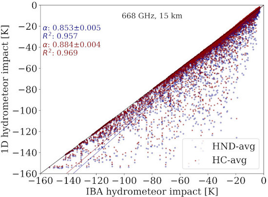
The correlations of the simulated brightness temperature between the IBA and the two different 1D calculation modes (see Section 3) at slant view, i.e., HND-avg (in dark blue) and HC-avg (dark red), are found in Figure 6. In contrast to the comparison between the 3D and IBA simulations (see Figure 4), this comparison introduces a significant scatter, especially at a frequency of 668 GHz. Still, most of the points are bundled around the one-to-one line, mainly in the case of HC-avg (and for below 80 K) and rather good linear relations were found between the IBA and 1D, with values being greater than 0.957. Altogether, performing 1D simulations led to an overestimation of the hydrometeor impact, with the overestimation found to be larger at the highest frequency (668 GHz) and at the largest footprint size (15 km). Only for a footprint size of 6 km and a frequency of 186.3 GHz, was a rather good agreement found between the two calculation modes, where the smallest scatter was found with values of about 0.997 and 0.999 for HND-avg and HC-avg, respectively. Furthermore, between the two 1D calculations modes, discrepancies are larger for HND-avg compared to HC-avg. Note here that in the case of HC-avg, for rather low values of the hydrometeor impact (above K), the data points are above the one-to-one line.
Figure 7 displays the corresponding histograms of the differences in brightness temperature between IBA and 1D calculations modes (at slant view) and gives an insight into the beam-filling effect. The discrepancies associated with the HND-avg (in dark blue) are concentrated on the left, and hence, are characterized by a right-skewed distribution, with a rather long tail, for both frequencies and footprints. Additionally, the peaks of the distributions lay always to the right from the zero difference line (marked by the black line), signifying a consistently positive beam-filling effect, leading to a mean error up to 1.549 K at 186.3 GHz and one up to 5.966 K at 668 GHz; the corresponding RMSEs are 3.973 K and 13.13 K, respectively. To summarize, the beam-filling error induced by neglecting domain heterogeneities from the slant view can be as large as ≈14 K at the highest frequency, defined by the 1.5 times the interquartile range (see the right arm of the whisker box in Figure 7d). Note here that the outliers can be as large as ≈40 K at 168.3 GHz and even more than 50 K at 668 GHz, but in the graphs results are presented up to a BF effect of about 15 K for better illustrative reasons.
In the same direction are the findings for the HC-avg at 668 GHz; i.e., a right-skewed distribution was identified that is characterized by a long tail towards the right. However, the magnitude of the BF effect is less pronounced, with a mean error (RMSE) of 1.550 (5.737) K at a footprint size of 6 km and a mean error (RMSE) of 4.070 (10.76) K at a footprint size of 15 km. On the contrary, at a frequency of 186.3 GHz, the histograms of differences in approximate a normal distribution quite well, with a very short tail (especially at a 6 km footprint size). Accordingly, the mean (RMSE) value of the BF is (1.047) K at 6 km footprint size and is 0.160 (2.123) K at 15 km. For both frequencies and footprint sizes in Figure 7, one can clearly see that, in this case (HC-avg), the peaks of the histograms are always located to the left of the zero difference line. In other words, at low values of the hydrometeor impact (above K), conducting 1D radiative transfer simulations by means of a HC-avg approach can lead to a negative BF effect (an underestimation of the simulated brightness temperature).
For radiative transfer simulations at nadir, the same behavior was found. However, conducting 1D simulations (both HND-avg and HC-avg) led to slightly smaller BF errors compared to the simulations at slant view. From nadir, the field of view of the sensor is smaller (on average), and therefore, so is the heterogeneity along this path. Consequently, slightly better linear correlations were found between IBA and both 1D simulation modes, with 1D simulations explaining above ≈96% and 97% of the variance in the simulated for HND-avg and HC-avg, respectively.
4.2.2. Mid-Latitudes
In the mid-latitudes, the errors induced by neglecting domain heterogeneities followed the same trends as in the tropics; i.e., the errors were found to be larger at the largest footprint size (15 km), at the highest frequency (668 GHz), and from slant view rather than nadir. Thus, we report only the slight differences, and for details the reader is referred to Table 2. To begin with, compared to the tropics, the simulated hydrometeor’s impact is considerably lower, with its values being above K and K at 186.3 GHz and at 668 GHz, respectively. Clouds over mid-latitudes were found at lower altitudes, and thus, are characterized by lower ice hydrometeor content. Consequently, the beam-filling effect was found to be significantly smaller with a mean error below ≈0.9 K and a RMSE below 2.437 K. Regarding the two 1D calculation modes, both HND-avg and HC-avg produce comparable BF effects, with HND-avg leading to the largest error, only at 186.3 GHz. At 668 GHz, the opposite holds true.
The histograms of the BF effect are described by narrower distributions compared to the case of tropics. As an example, Figure 8 depicts the corresponding histograms in the case of simulations from slant view. For both footprint sizes and both frequencies, only right-skewed distributions were found for both HND-avg and HC-avg. Recall here that in the case of the tropics and a frequency of 186.3 GHz, the corresponding histograms for HC-avg were better represented by normal distributions. Considering the low hydrometeor impact and the small magnitude of the BF error, the probability density at smaller values is higher compared to that in the tropics (see the peaks for each mode in Figure 7). An exception is posed by the distribution of the BF effect at a frequency of 186.3 GHz with a footprint size of 15 km in the case of HND-avg only, where, apart from the high peak that is located left from the zero difference line, a much lower peak is clearly visible at values of the BF error close to 1.6 K. The same behavior is visible in the histograms of the BF error from nadir view, but the two peaks are slightly closer to each other (not shown here). For the two 1D calculation modes, both HND-avg and HC-avg produce comparable beam-filling effects, with HND-avg leading to the largest error only at 186.3 GHz. At 668 GHz, the opposite holds true.
4.3. Total Effect
As we already mentioned, the comparison between the full 3D and the 1D simulations introduces the total effect; i.e., the combined impact of the horizontal photon transport and beam-filling effect. Table 3 compiles the corresponding statistics. One can clearly see that on average, the total effect can be seen as the sum of the two effects (comparing Table 3 with Table 1 and Table 2), but this is no surprise considering their linear relation (see Equation 7). For very small values of the hydrometeor impact (below 10 K), there is a rather good agreement between the calculation modes. However, the differences increase at higher values of the . Overall, the total effect follows the same behavior as the BF effect, and consequently, any repetition is redundant. For details, the reader is referred to Table 3 and Section 4.2. From this, in addition to the small horizontal photon effect, one can conclude that the total radiative effect is always driven by the BF one.
On the whole, conducting 1D simulations and neglecting the 3D heterogeneous atmosphere over the field of view of the sensor can lead to substantial 3D effects, with a mean error (RMSE) up to 1.738 (4.425) K at 186.3 GHz and one up to 6.337 (13.88) K at 668 GHz.
4.4. Empirical Correction Scheme
Each of the aforementioned comparisons among the different calculation modes, i.e., 3D against IBA (HPT effect), IBA against 1D (BF effect), and 3D in contrast to 1D (total effect), can be described by a linear regression model. To that end, the ordinary least squares regression technique was utilized, whereby the following simple model function was applied:
This technique yields the projection line, whereby each of the regressors x (IBA or 1D) are correlated to a maximal degree with y (3D or IBA) and supplies the slopes, which reduce the error in the prediction of y. Results are compiled in Table 1, Table 2 and Table 3. As described above, an excellent linear correlation was obtained from all the comparisons, but with a significant scatter, mainly in the case of the total and the beam-filling effects, which strongly depend on the frequency, footprint size, and slant path. To that end, the slope of the latter model can be seen as a multiplication correction factor (hereafter slope correction) that forces the errors in the prediction of the simulated brightness temperature by each approximation (IBA or 1D) to be more symmetric. Note here that the impact of such a slope correction at mm/sub-mm wavelengths is more pronounced when the 3D effects are larger. Accordingly, at the lowest frequency, smallest footprint size, and from nadir view, it induces only a minor improvement of about 0.1 K.
Starting with the total effect, both 1D simulation modes can explain at least 95.2% (see Table 3) of the variance in the brightness temperature field resulting from the full 3D mode, with the HC-avg method leading to slightly better results. Consequently, the slope correction diminishes the RMSE by up to 3.2 K, chiefly at a footprint size of 15 km and a frequency of 668 GHz, where the largest effect was found. Overall, the RMSE of the combined effect introduced by conducting 1D simulations was improved from K to K in the case of HND-avg and from K to K in the case of HC-avg, where RMSE denotes the corrected RMSE. In the same direction are the findings for the beam-filling effect, in which the slope correction can lead to an improvement up to ≈3 K. On the contrary, the slope correction is negligible (below 0.1 K) when it comes from the horizontal photon transport effect. In fact, IBA simulations are able to explain nearly 100% of the variance in the 3D simulations, and only minor discrepancies were recorded (see Section 4.1). For details, the reader is referred to Table 1, Table 2 and Table 3.
5. Discussion
By confronting the full 3D with 1D simulations, one can explore the errors induced by neglecting the 3D aspect of the atmosphere and give rise to the so-called 3D effects—the beam-filling and the horizontal photon transport effect. In order to provide estimates of the magnitudes of these two effects individually and point out which is the dominant one at mm/sub-mm wavelengths, we additionally conducted simulations according to the independent beam approximation.
5.1. The Horizontal Photon Transport Effect
At mm/sub-mm wavelengths, the single scattering albedo of ice hydrometeors is very high, meaning that their interaction with radiation is mostly governed by scattering. In other words, the multiple scattering process is enhanced, while absorption, and hence, emission, is of less importance. Accordingly, one could assume that the horizontal photon transport effect, which is driven by multiple-scattering process, would be enhanced compared to other studies at lower frequencies, where the issue under investigation was liquid water clouds or precipitation that are characterized by smaller single scattering albedo [39,87]. On the contrary, the comparison between the full 3D radiative transfer simulations (3D mode) and the independent beam approximation (IBA mode) reveals no considerable discrepancies, with IBA simulations introducing a small overestimation and mostly random errors. In short, the mean HPT error is below 0.433 K, with a RMSE below 1.964 K, confirming the findings of Davis et al. [44] over the same frequencies. Particularly, IBA simulations (without considering the antenna pattern) produce somewhat smoother results compared to 3D simulations that could lead to both positive and negative horizontal photon transport effects. These effects, which can be as large as K, e.g., see Figure 3c, are subject to the 3D structures of clouds, especially at the areas with a large gradient in hydrometeor content. However, the integration over the antenna pattern of the satellite, which is characterized by a large full width at half maximum (6 and 15 km), neutralizes the effect and significantly decreases its size.
The magnitude of this effect strongly depends on the frequency, the footprint size, and the observation angle of the satellite. In fact, the larger the frequency, the larger the effect. Larger frequency means that the hydrometeors are characterized by a larger scattering cross section, which potentially leads to an increasing number of multiple-scattering events, and thus, an increasing probability for a photon traveling between neighboring columns with different optical properties. In addition, decreasing the footprint size results in an increase of the HPT effect because the variability in optical properties is resolved by smaller scales. In principle, the magnitude of the HPT effect is less pronounced from nadir view compared to slant view. This can be explained by the fact that the effective photon path length is (on average) decreased, and consequently, so is the number of scattering events. However, this is true only in the tropics. In the mid-latitudes, the mean errors owing to the neglection of the HPT were found to be slightly larger for nadir viewing instruments. This can be explained by the fact that the differences between the 3D and IBA modes are centered closer to the zero difference line (see Figure 5). In terms of the RMSE, the HPT effect is still larger for the slant path—with those instruments operating at the lowest frequency and being characterized by the largest footprint size (ICI- and SSMIS-wise) being the exception; recall here that for all across-track instruments, we only refer to their nominal resolution at nadir. For the solar spectrum, similar results have been reported by Barlakas [22] and O’Hirok and Gautier [88]. They found that such behavior is subject to the gradient in hydrometeor content and the observational geometry and could be attributed to photon trapping and shadowing effects. Last but not least, the HPT in mid-altitudes is less pronounced compared to the tropics. Clouds containing ice in mid-latitudes are located at lower altitudes and are characterized by lower ice water content. In addition, at lower altitudes, the absorption by water vapor is of great importance for the frequencies under investigation, and hence, the number of scattering events is rather low, which further diminishes the magnitude of the HPT effect.
5.2. The Beam-Filling Effect
For both tropics and mid-latitudes, the beam-filling errors induced by conducting 1D radiative transfer simulations from both slant and nadir views increase with increasing frequency. However, increasing the footprint size of the sensor results in an increase of the magnitude of the BF effect. This can be explained by the fact that we resolve the variability in optical properties at larger scales. Overall, performing 1D simulations over all-sky conditions leads to a systematic overestimation of the hydrometeor impact, with mean error (RMSE) up to 1.549 (3.973) K at 186.3 GHz and one up to 5.966 (13.13) K at 668 GHz. This overestimation, which is driven by the non-linear relationship between the brightness temperature and the hydrometeor content in the field of view of the sensor [3], further supports the findings of Davis et al. [44].
At rather low values of the hydrometeor impact, i.e., below K, the errors prompted by neglecting domain heterogeneities can produce both positive and negative beam-filling effects (see Figure 6). At the frequencies under investigation, the sign of the BF effect depends on the vertical and horizontal variability (gradient) of the hydrometeor content, and consequently, the vertical and horizontal placement of clouds along the field of view of a sensor. In brief, by averaging inhomogeneities over the large footprint sizes, especially at slant view instruments (AMSU-B-, ATMS-, and MHS-wise), could potentially lead to values of ice water path that can be high enough to be at the non-linear regime, and 1D simulations could yield higher hydrometeor impact compared to IBA simulations for a given ice water path [3]. Similar findings have been found by Davis et al. [44] and Lafont and Guillemet [36]. Davis et al. [44] reported a negative BF effect in the case of mm wavelengths (190 GHz) at low values of the hydrometeor impact (below ≈7 K). In addition, Lafont and Guillemet [36] demonstrated that for convective precipitating clouds, the BF effect can be between to 10 K strongly depending on cloud cover. Between HND- and HC-avg calculation modes, the latter one mostly leads to negative values of the BF effect and to an overall smaller bias. One can clearly see in Figure 7 and Figure 8 that the peaks of the histograms for the latter case are always located to the left of the zero difference line. Averaging the hydrometeor content over the field of view of the sensor, and then determining the hydrometeor number density, could potentially induce particles that are smaller in size. Consequently, for a given frequency, this implies particles characterized by smaller scattering cross section. In other words, HC-avg results in hydrometeors that are more absorbing (enhanced emission) and by confronting them to the IBA counter part brightness temperature could lead to the negative sign of the BF effect. For instance, by directly applying the antenna pattern to the hydrometeor number density (HND-avg), we do not alter the size of hydrometeors, and therefore, the impact of the aforementioned non-linearity is more pronounced.
5.3. Total Effect and Implications for Retrievals and Data Assimilation
The total effect prompted by ignoring 3D heterogeneities was found to be consistent with the beam-filling effect. Moreover, with the paucity of the horizontal photon transport effect, we could conclude that, for mm/sub-mm wavelengths, the beam-filling one drives the 3D radiative effects.
Our analysis implies that observations of cloud ice, and as a result, ice retrievals based on all the aforementioned instruments, are and will be unfavorably contaminated by the beam-filling effect. As we mentioned above, the BF effect, and thus, the 3D effects overall depend on the view (slant or nadir), the size of the footprint, and the frequency, with the latter one causing the largest impact. Thus, ICI-based retrievals will be the ones mostly affected by 3D effects characterized by RMSEs of up to ≈4.4 K at 186.3 GHz and ≈14 K at 668 GHz. The same stands for any future satellite mission with instruments operating at sub-mm wavelengths, which will be described by even smaller footprint size (6 km), whereby the corresponding RMSE could be as large as ≈8.2 K. Among the current instruments that operate at a frequency of 186.3 GHz and are characterized by a footprint of about 15 km (AMSU-B, ATMS, and MHS at nadir only and SSMIS), SSMIS-based retrievals are marginally subject to the largest error (up to ≈1.2 K more). GMI-wise retrievals, which are supplied by a channel at ≈186.3 GHz and characterized by the smallest footprint size, are the ones affected least by 3D effects; the RMSE is below ≈2.6 K. These results allow us to draw similar conclusions for the upcoming Microwave Imager (MWI) mission that will fly together with ICI on Metop-SG. This instrument is a conically scanning radiometer with five channels at ≈183 GHz (among others). Even though MWI is characterized by a footprint of about 10 km, we assume that the beam-filling RMSE will be around ≈3.5 K, especially in scenes over intertropical latitudes.
In passive MW retrievals of precipitation, the errors induced owing to the use of 1D plane-parallel simulations have been investigated by plenty of former studies. Consequently, correction schemes have been developed over the last years consisting of a static factor [30,36], a dynamic adjustment [89], and diminishing the error by employing the channel with the highest resolution [34,38]. In this study, a first attempt was made to mitigate 3D effects by applying a statistical correction scheme by means of a multiplication factor. On the basis of the excellent linear correlation among the different calculation modes, we wield the ordinary least squares regression method to derive the slope of the simple linear model as the multiplication factor to induce a more symmetric 3D error. Accordingly, the slope correction diminished the RMSE by up to 3.2 K, particularly at the largest frequency and footprint size.
Finally, our findings are also relevant to all-sky data assimilation. In data assimilation, sub-grid variability (domain heterogeneities) is only crudely taken into account. Accordingly, radiative transfer simulations are conducted by means of a 1D plane-parallel approximation. In addition, considering the much larger scales of the model domain, a considerable 3D effect is expected. For instance, for the frequencies considered so far (below ≈190 GHz), the area-averaged precipitation is systematically underestimated [90]. ICI holds a strong potential to extend the scope of data assimilation towards the sub-mm region. Accordingly, our results provide a first insight of the size of the 3D effect and further explore the use of an empirical correction scheme, which could potentially yield a more symmetric error.
5.4. Implications to Future Satellite Instruments
The significant 3D effects discussed above should be considered in the design of future satellite missions. Let us consider, for example, the highest frequency channel of ICI; i.e., 664 GHz. For this channel, the noise requirement is 1.6 K [10]. For observations over tropical latitudes that are substantially affected by clouds, there is also a modeling uncertainty of ≈9.5 K, even if a correction is applied (see Table 3). The two error sources discussed are independent and the total uncertainty is ≈9.6 K.
A MW radiometer operating at the same frequency, yet with a much smaller footprint size, would be subject to smaller modeling uncertainties. For the case of a 6 km footprint, the matching estimate in Table 3 is 6.0 K. An instrument with such a footprint size can be achieved. In fact, the 664 GHz channel of ICI is designed to have the same footprint size as the 183.31 GHz ones, while the antenna size, in principle, allows for a footprint of 6 km. For an across-track scanning instrument, an effective antenna size of 1 dm would suffice to obtain 6 km resolution over a considerable swath width. Anyhow, assuming that other technical characteristics are unchanged, observations for a 6 km footprint would have a noise level of 4 K (a factor of 2.5 higher), leading to total uncertainty of 7.2 K.
Overall, a more accurate cloud retrieval can be performed at 6 km resolution than at 15 km, despite that the instrument noise is higher. One could argue that a noise of 4 K is too high for a meaningful retrieval of humidity. However, for clear-sky conditions the 6 km observations can be averaged to 15 km resolution and the noise is brought back to 1.6 K. An instrument having a 6 km resolution will require a faster rotating antenna, which will cause technical challenges, and will generate larger data volumes. Nevertheless, aiming for smaller footprint sizes should be considered, since it will provide cloud information with both higher spatial resolution and better precision.
Future satellite missions could also explore the combined use of an active instrument (e.g., similar to CloudSat) in a constellation with a passive radiometer operating at sub-mm wavelengths. The high vertical and horizontal resolution of the active sensor could supply the passive retrievals with a more detailed view of sub-grid variability of ice hydrometeors. Such a combination gives, in addition, increased information on microphysical properties of ice hydrometeors [91].
6. Conclusions
By means of the Atmospheric Radiative Transfer Simulator (ARTS), a study has been carried out in order to explore the errors prompted by omitting three-dimensional (3D) radiative transfer at millimeter/sub-millimeter (mm/sub-mm) wavelengths. This study gives an insight of the 3D effects, i.e., beam-filling and horizontal photon transport effects, which contaminate cloud ice retrievals from both current and forthcoming satellite missions, with a focus on the Ice Cloud Imager (ICI). Accordingly, forward radiative transfer simulations were carried out for two incident angles at the ground, i.e., 53 (slant view) and 0 (nadir view); at two frequencies (186.3 GHz and 668 GHz); and with two footprint sizes, i.e., 6 km and 15 km, over several tropical and mid-latitude cloud scenes. The 3D synthetic scenes have been generated from two-dimensional (2D) CloudSat (Cloud Satellite) observations utilizing a stochastic approach.
By conducting a comprehensive statistical analysis over randomly sampled scenes, we demonstrated that, for mm/sub-mm wavelengths:
- The horizontal photon transport effect is rather small, and thus, the errors induced by neglecting the 3D heterogeneities of clouds can be mostly linked to the beam-filling effect. In fact, conducting radiative transfer simulations by means of an independent beam approximation (IBA) induces a slight overestimation and chiefly random errors. Accordingly, the realistic but computational expensive 3D radiative transfer simulations could be excluded from retrievals of current and proposed satellite missions, providing the fact that the bias of the forward model is adjusted by a correction factor between 0.1 and 1 K.
- On the contrary, performing one-dimensional (1D) radiative transfer simulations following the plane-parallel assumption divulges a significant beam-filling effect that increases primarily with frequency, and secondly, with footprint size and slant path. On this basis, we conclude that ice cloud retrievals that supply the optimal estimation approach (also known as 1D variational inversion algorithm, 1DVAR) by current or future satellite instruments are and will be adversely contaminated by the beam-filling effect. Consequently, this promotes the use of alternative methods, which are based on retrieval databases and utilize IBA simulations [92]. In fact, such a retrieval database has been suggested for the upcoming ICI operational product [10].
- In case IBA simulations are still not computationally feasible, then, among the two different 1D calculations modes, i.e., (a) HND-avg that employs the mean of the 3D hydrometeor number density field and (b) HC-avg that utilizes the 1D hydrometeor number density derived from the mean hydrometeor content, the latter one is preferable, since it leads to slightly smaller systematic errors—up to ≈1.9 K and a root mean square error (RMSE) of about 2.3 K at a frequency of 668 GHz with a footprint size of 15 km at which the largest errors were reported.
- Our findings indicate that 1DVAR retrievals and data assimilation at sub-mm wavelengths will be largely affected by 3D effects. In our framework, a simple statistical correction scheme by means of a multiplication factor has been developed that compels the errors induced by neglecting domain heterogeneities to be more symmetric. This multiplication factor is the slope of the excellent linear correlation between 3D and 1D simulations. Under these circumstances, the RMSE of the 3D effect is reduced by up to 3.2 K. Note here that this was a first attempt towards a correction scheme for 1DVAR retrievals, with a potential use in all-sky assimilation; diminution of the 3D effect along the field of view of ICI at mm/sub-mm wavelengths instructs a separate study including all the channels of ICI, and thus, it was beyond the scope of this paper.
- The considerable 3D effects reported here at sub-mm wavelengths with a footprint size of 15 km should be acknowledged for any future sensor design. Even though a radiometer operating at these wavelengths and characterized by smaller footprint size does not exist still, its cloud observations will be available in a finer spatial resolution and with a better overall precision considering the much smaller modeling uncertainties.
Future research could aim at further exploring the use of the current empirical correction scheme, or the development of a new correction scheme for the beam-filling effect at mm/sub-mm wavelengths. In this work, due to the limitation in scattering databases that cover particle orientation at mm/sub-mm wavelengths, only randomly oriented hydrometeors have been considered. A subsequent step should be to include particle orientation in order to explore polarization effects that were introduced first by [44], and the recently published work by Brath et al. [93] makes such extension feasible.
Author Contributions
Both V.B. and P.E. conceived and refined the overall structure of the investigation. V.B. carried out the simulations, refined the data analysis, and wrote the manuscript. Both authors contributed to the interpretation of the results and to the manuscript’s improvement. All authors have read and agreed to the published version of the manuscript.
Funding
The work of Vasileios Barlakas at Chalmers University of Technology is funded by a EUMETSAT fellowship program.
Acknowledgments
We thank our colleague, Simon Pfreundschuh, for the many thoughtful comments that led to the improvement of the manuscript.
Conflicts of Interest
The authors declare no conflict of interest.
Abbreviations
| 1D | one-dimensional |
| 1DVAR | 1D variational inversion algorithm |
| 2D | two-dimensional |
| 3D | three-dimensional |
| AMSR | Advanced Microwave Scanning Radiometer |
| AMSU-B | Advanced Microwave Sounding Unit-B |
| ARTS | Atmospheric Radiative Transfer Simulator |
| ARTS-MC | ARTS Monte Carlo |
| ATMS | Advanced Technology Microwave Sounder |
| BF | beam-filling |
| CIWSIR | Cloud Ice Water Submillimeter Imaging Radiometer |
| CloudSat | Cloud Satellite |
| CoSSIR | Compact Scanning Submillimeter-wave Imaging Radiometer |
| CPR | cloud profiling radar |
| DISORT | Discrete Ordinates Radiative Transfer Program for a Multi-Layered Plane-Parallel Medium |
| ECMWF | European Centre for Medium-Range Weather Forecasts |
| EOS-MLS | Earth Observing System Microwave Limb Sounder |
| ERA-Interim | ECMWF reanalysis data |
| EUMETSAT | European Organization of Meteorological Satellites |
| F07 | Field et al. [75] |
| GMI | GPM microwave imager |
| GPM | Global Precipitation Mission |
| HC | hydrometeor content |
| HC-avg | HC averaging |
| HND | hydrometeor number density |
| HND-avg | HND averaging |
| HPT | horizontal photon transport |
| IAAFT | Iterative Amplitude Adjusted Fourier Transform |
| IBA | independent beam approximation |
| ICA | independent column approximation |
| ICI | Ice Cloud Imager |
| ISMAR | International Submillimetre Airborne Radiometer |
| IWC | ice water content |
| LWC | liquid water content |
| Metop-SG | Meteorological Operational Satellite-Second Generation |
| MH97 | McFarquhar and Heymsfield [72] |
| MHS | Microwave Humidity Sounder |
| mm | millimeter |
| MW | microwave |
| MWI | Microwave Imager |
| NWP | numerical weather prediction |
| Odin-SMR | Odin-Sub-Millimetre Radiometer |
| PSD | particle size distributions |
| RMSE | root mean square error |
| RMSE | RMSE corrected by the slope of the regression line |
| RWC | rain water content |
| SMILES | Superconducting Submillimeter-Wave Limb-Emission Sounder |
| SSMIS | Special Sensor Microwave Imager/Sounder |
| sub-mm | sub-millimeter |
| Suomi NPP | Suomi National Polar-orbiting Partnership |
| TESSEM2 | Tool to Estimate Sea Surface Emissivity from Microwave to sub-Millimeter waves |
| TMI | TRMM Microwave Imager |
| TRMM | Tropical Rainfall Measuring Mission |
References
- Duncan, D.I.; Eriksson, P. An update on global atmospheric ice estimates from satellite observations and reanalyses. Atmos. Chem. Phys. 2018, 18, 11205–11219. [Google Scholar] [CrossRef] [Green Version]
- Waliser, D.E.; Li, J.L.F.; Woods, C.P.; Austin, R.T.; Bacmeister, J.; Chern, J.; Del Genio, A.; Jiang, J.H.; Kuang, Z.; Meng, H.; et al. Cloud ice: A climate model challenge with signs and expectations of progress. J. Geophys. Res. Atmos. 2009, 114. [Google Scholar] [CrossRef]
- Buehler, S.A.; Jiménez, C.; Evans, K.F.; Eriksson, P.; Rydberg, B.; Heymsfield, A.J.; Stubenrauch, C.J.; Lohmann, U.; Emde, C.; John, V.O.; et al. A concept for a satellite mission to measure cloud ice water path, ice particle size, and cloud altitude. Q. J. R. Meteorol. Soc. 2007, 133, 109–128. [Google Scholar] [CrossRef] [Green Version]
- Geer, A.J.; Lonitz, K.; Weston, P.; Kazumori, M.; Okamoto, K.; Zhu, Y.; Liu, E.H.; Collard, A.; Bell, W.; Migliorini, S.; et al. All-sky satellite data assimilation at operational weather forecasting centres. Q. J. R. Meteorol. Soc. 2018, 144, 1191–1217. [Google Scholar] [CrossRef]
- Geer, A.J.; Baordo, F.; Bormann, N.; Chambon, P.; English, S.J.; Kazumori, M.; Lawrence, H.; Lean, P.; Lonitz, K.; Lupu, C. The growing impact of satellite observations sensitive to humidity, cloud and precipitation. Q. J. R. Meteorol. Soc. 2017, 143, 3189–3206. [Google Scholar] [CrossRef]
- Stephens, G.L.; Vane, D.G.; Boain, R.J.; Mace, G.G.; Sassen, K.; Wang, Z.; Illingworth, A.J.; O’connor, E.J.; Rossow, W.B.; Durden, S.L.; et al. The CloudSat mission and the A-train. Bull. Am. Meteorol. Soc. 2002, 83, 1771–1790. [Google Scholar] [CrossRef] [Green Version]
- Draper, D.W.; Newell, D.A.; Wentz, F.J.; Krimchansky, S.; Skofronick-Jackson, G.M. The Global Precipitation Measurement (GPM) Microwave Imager (GMI): Instrument overview and early on-orbit performance. IEEE IEEE J. Sel. Topics Appl. Earth Observ. Remote Sens. 2015, 8, 3452–3462. [Google Scholar] [CrossRef]
- Birman, C.; Mahfouf, J.F.; Milz, M.; Mendrok, J.; Buehler, S.A.; Brath, M. Information content on hydrometeors from millimeter and sub-millimeter wavelengths. Tellus 2017, 69. [Google Scholar] [CrossRef]
- Accadia, C.; Schlüssel, P.; Phillips, P.L.; Wilson, J.J.W. The EUMETSAT Polar System-Second Generation (EPS-SG) micro-wave and sub-millimetre wave imaging missions. SPIE Proc. 2013. [Google Scholar] [CrossRef]
- Eriksson, P.; Rydberg, B.; Mattioli, V.; Thoss, A.; Accadia, C.; Klein, U.; Buehler, S.A. Towards an operational Ice Cloud Imager (ICI) retrieval product. Atmos. Meas. Tech. 2020, 13, 53–71. [Google Scholar] [CrossRef] [Green Version]
- Brath, M.; Fox, S.; Eriksson, P.; Harlow, R.C.; Burgdorf, M.; Buehler, S.A. Retrieval of an ice water path over the ocean from ISMAR and MARSS millimeter and submillimeter brightness temperatures. Atmos. Meas. Tech. 2018, 11, 611–632. [Google Scholar] [CrossRef] [Green Version]
- Fox, S.; Mendrok, J.; Eriksson, P.; Ekelund, R.; O’Shea, S.J.; Bower, K.N.; Baran, A.J.; Harlow, R.C.; Pickering, J.C. Airborne validation of radiative transfer modeling of ice clouds at millimetre and sub-millimetre wavelengths. Atmos. Meas. Tech. 2019, 12, 1599–1617. [Google Scholar] [CrossRef] [Green Version]
- Evans, K.F.; Wang, J.R.; O’C Starr, D.; Heymsfield, G.; Li, L.; Tian, L.; Lawson, R.P.; Heymsfield, A.J.; Bansemer, A. Ice hydrometeor profile retrieval algorithm for high-frequency microwave radiometers: application to the CoSSIR instrument during TC4. Atmos. Meas. Tech. 2012, 5, 2277–2306. [Google Scholar] [CrossRef] [Green Version]
- Eriksson, P.; Rydberg, B.; Sagawa, H.; Johnston, M.S.; Kasai, Y. Overview and sample applications of SMILES and Odin-SMR retrievals of upper tropospheric humidity and cloud ice mass. Atmos. Chem. Phys. 2014, 14, 12613–12629. [Google Scholar] [CrossRef] [Green Version]
- Cahalan, R.F.; Ridgway, W.; Wiscombe, W.J.; Bell, T.L.; Snider, J.B. The albedo of fractal stratocumulus clouds. J. Atmos. Sci. 1994, 51, 2434–2455. [Google Scholar] [CrossRef]
- Várnai, T.; Davies, R. Effects of cloud heterogeneities on shortwave radiation: comparison of cloud-top variability and internal heterogeneity. J. Atmos. Sci. 1999, 56, 4206–4224. [Google Scholar] [CrossRef]
- Benner, T.C.; Evans, K.F. Three-dimensional solar radiative transfer in small tropical cumulus fields derived from high-resolution imagery. J. Geophys. Res. 2001, 106, 14975–14984. [Google Scholar] [CrossRef] [Green Version]
- Barlakas, V.; Macke, A.; Wendisch, M. SPARTA—Solver for Polarized Atmospheric Radiative Transfer Applications: Introduction and application to Saharan dust fields. J. Quant. Spectrosc. Radiat. Transfer 2016, 178, 77–92. [Google Scholar] [CrossRef] [Green Version]
- Di Giuseppe, F.; Tompkins, A.M. Effect of spatial organisation on solar radiative transfer in three-dimensional idealized stratocumulus cloud fields. J. Atmos. Sci. 2003, 60, 1774–1794. [Google Scholar] [CrossRef]
- Marshak, A.; Davis, A. 3D Radiative Transfer in Cloudy Atmospheres; Springer: Berlin/Heidelberg, Germany, 2005. [Google Scholar] [CrossRef]
- Scheirer, R.; Macke, A. On the accuracy of the independent column approximation in calculating the downward fluxes in the UVA, UVB, and PAR spectral ranges. J. Geophys. Res. 2001, 106, 14301–14312. [Google Scholar] [CrossRef] [Green Version]
- Barlakas, V. A new three-dimensional vector radiative transfer model and applications to Saharan dust fields. Ph.D. Thesis, Leipzig University, Leipzig, Germany, 2016. [Google Scholar]
- Davis, A.B.; Garay, M.J.; Xu, F.; Qu, Z.; Emde, C. 3D radiative transfer effects in multi-angle/multispectral radio-polarimetric signals from a mixture of clouds and aerosols viewed by a non-imaging sensor. SPIE Proc. 2013. [Google Scholar] [CrossRef]
- Stap, F.; Hasekamp, O.; Emde, C.; Röckmann, T. Influence of 3D effects on 1D aerosol retrievals in synthetic, partially clouded scenes. J. Quant. Spectrosc. Radiat. Transfer 2016, 170, 54–68. [Google Scholar] [CrossRef]
- Stap, F.A.; Hasekamp, O.P.; Emde, C.; Röckmann, T. Multiangle photopolarimetric aerosol retrievals in the vicinity of clouds: Synthetic study based on a large eddy simulation. J. Geophys. Res. Atmos. 2016, 121, 12914–12935. [Google Scholar] [CrossRef] [Green Version]
- Várnai, T.; Marshak, A.; Yang, W. Multi-satellite aerosol observations in the vicinity of clouds. Atmos. Chem. Phys. 2013, 13, 3899–3908. [Google Scholar] [CrossRef] [Green Version]
- Wen, G.; Marshak, A.; Levy, R.C.; Remer, L.A.; Loeb, N.G.; Varnai, T.; Cahalan, R.F. Improvement of MODIS aerosol retrievals near clouds. J. Geophys. Res. Atmos. 2013, 118, 9168–9181. [Google Scholar] [CrossRef]
- Alexandrov, M.D.; Cairns, B.; Emde, C.; Ackerman, A.S.; van Diedenhoven, B. Accuracy assessments of cloud droplet size retrievals from polarized reflectance measurements by the research scanning polarimeter. Remote Sens. Environ. 2012, 125, 92–111. [Google Scholar] [CrossRef] [Green Version]
- Cornet, C.; Labonnote, C.L.; Waquet, F.; Szczap, F.; Deaconu, L.; Parol, F.; Vanbauce, C.; Thieuleux, F.; Riédi, J.C. Cloud heterogeneity on cloud and aerosol above cloud properties retrieved from simulated total and polarized reflectances. Atmos. Meas. Tech. 2018, 11, 3627–3643. [Google Scholar] [CrossRef] [Green Version]
- Wilheit, T.T.; Chang, A.T.C.; Rao, M.S.; Rodgers, E.B.; Theon, J.S. A satellite technique for quantitatively mapping rainfall rates over the oceans. J. Appl. Meteor. 1977, 16, 551–560. [Google Scholar] [CrossRef] [Green Version]
- Weinman, J.A.; Davies, R. Thermal microwave radiances from horizontally finite clouds of hydrometeors. J. Geophys. Res. Oceans 1978, 83, 3099–3107. [Google Scholar] [CrossRef]
- Kummerow, C.; Weinman, J.A. Determining microwave brightness temperatures from precipitating horizontally finite and vertically structured clouds. J. Geophys. Res. Atmos. 1988, 93, 3720–3728. [Google Scholar] [CrossRef]
- Haferman, J.L.; Krajewski, W.F.; Smith, T.F.; Sánchez, A. Radiative transfer for a three-dimensional raining cloud. Appl. Opt. 1993, 32, 2795–2802. [Google Scholar] [CrossRef] [PubMed]
- Petty, G.W. Physical retrievals of over-ocean rain rate from multichannel microwave imagery. Part I: Theoretical characteristics of normalized polarization and scattering indices. Meteorol. Atmos. Phys. 1994, 54, 79–99. [Google Scholar] [CrossRef]
- Liu, Q.; Simmer, C. Polarization and intensity in microwave radiative transfer. Beitr. Phys. Atmosph. 1996, 69, 535–545. [Google Scholar]
- Lafont, D.; Guillemet, B. Subpixel fractional cloud cover and inhomogeneity effects on microwave beam-filling error. Atmos. Res. 2004, 72, 149–168. [Google Scholar] [CrossRef]
- Roberti, L.; Haferman, J.; Kummerow, C. Microwave radiative transfer through horizontally inhomogeneous precipitating clouds. J. Geophys. Res. Atmos. 1994, 99, 16707–16718. [Google Scholar] [CrossRef]
- Bauer, P.; Schanz, L.; Roberti, L. Correction of three-dimensional effects for passive microwave remote sensing of convective clouds. J. Appl. Meteorol. 1998, 37, 1619. [Google Scholar] [CrossRef]
- Kummerow, C. Beamfilling errors in passive microwave rainfall retrievals. J. Appl. Meteorol. 1998, 37, 356–370. [Google Scholar] [CrossRef]
- Kroodsma, R.; Bilanow, S.; Ji, Y.; McKague, D. TRMM Microwave Imager (TMI) updates for final data version release. IEEE Trans. Geosci. Remote Sens. 2017, 1216–1219. [Google Scholar] [CrossRef]
- Dong, S.; Gille, S.T.; Sprintall, J.; Gentemann, C. Validation of the Advanced Microwave Scanning Radiometer for the Earth Observing System (AMSR-E) sea surface temperature in the Southern Ocean. J. Geophys. Res. 2006, 111. [Google Scholar] [CrossRef]
- Battaglia, A.; Simmer, C.; Czekala, H. Three-dimensional effects in polarization signatures as observed from precipitating clouds by low frequency ground-based microwave radiometers. Atmos. Chem. Phys. 2006, 6, 4383–4394. [Google Scholar] [CrossRef] [Green Version]
- Battaglia, A.; Saavedra, P.; Morales, C.A.; Simmer, C. Understanding three-dimensional effects in polarized observations with the ground-based ADMIRARI radiometer during the CHUVA campaign. J. Geophys. Res. Atmos. 2011, 116. [Google Scholar] [CrossRef] [Green Version]
- Davis, C.P.; Evans, K.F.; Buehler, S.A.; Wu, D.L.; Pumphrey, H.C. 3-D polarised simulations of space-borne passive mm/sub-mm midlatitude cirrus observations: a case study. Atmos. Chem. Phys. 2007, 7, 4149–4158. [Google Scholar] [CrossRef] [Green Version]
- Hogan, R.; Kew, S. A 3D stochastic cloud model for investigating the radiative properties of inhomogeneous cirrus clouds. Q. J. R. Meteorol. Soc. 2005, 131, 2585–2608. [Google Scholar] [CrossRef] [Green Version]
- Hong, G.; Heygster, G.; Notholt, J.; Weng, F.; Liu, Q. Simulations of microwave brightness temperatures at AMSU-B frequencies over a 3D convective cloud system. Int. J. Remote Sens. 2010, 31, 1781–1800. [Google Scholar] [CrossRef]
- Wu, D.L.; Jiang, J.H.; Davis, C.P. EOS MLS cloud ice measurements and cloudy-sky radiative transfer model. IEEE Trans. Geosci. Remote Sens. 2006, 44, 1156–1165. [Google Scholar] [CrossRef]
- Eriksson, P.; Buehler, S.; Davis, C.; Emde, C.; Lemke, O. ARTS, the atmospheric radiative transfer simulator, version 2. J. Quant. Spectrosc. Radiat. Transf. 2011, 112, 1551–1558. [Google Scholar] [CrossRef] [Green Version]
- Buehler, S.A.; Mendrok, J.; Eriksson, P.; Perrin, A.; Larsson, R.; Lemke, O. ARTS, the Atmospheric Radiative Transfer Simulator – version 2.2, the planetary toolbox edition. Geosci. Model Dev. 2018, 11, 1537–1556. [Google Scholar] [CrossRef] [Green Version]
- Vangasse, P.; Charlton, J.; Jarrett, M. Characterisation of the Advanced Microwave Sounding Unit, AMSU-B. Adv. Space Res. 1996, 17, 75–78. [Google Scholar] [CrossRef]
- Vila, D.; Ferraro, R.; Joyce, R. Evaluation and improvement of AMSU precipitation retrievals. J. Geophys. Res. Atmos. 2007, 112. [Google Scholar] [CrossRef] [Green Version]
- Sanò, P.; Panegrossi, G.; Casella, D.; Di Paola, F.; Milani, L.; Mugnai, A.; Petracca, M.; Dietrich, S. The Passive microwave Neural network Precipitation Retrieval (PNPR) algorithm for AMSU/MHS observations: description and application to European case studies. Atmos. Meas. Tech. 2015, 8, 837–857. [Google Scholar] [CrossRef] [Green Version]
- Kim, M.J.; Weinman, J.A.; Olson, W.S.; Chang, D.E.; Skofronick-Jackson, G.; Wang, J.R. A physical model to estimate snowfall over land using AMSU-B observations. J. Geophys. Res. Atmos. 2008, 113. [Google Scholar] [CrossRef] [Green Version]
- Tian, X.; Zou, X. ATMS- and AMSU-A-derived hurricane warm core structures using a modified retrieval algorithm. J. Geophys. Res. Atmos. 2016, 121, 12630–12646. [Google Scholar] [CrossRef] [Green Version]
- Xu, X.; Zou, X. A modified ice water path retrieval algorithm applicable to the ATMS. Tellus A 2019, 71, 1–14. [Google Scholar] [CrossRef] [Green Version]
- Stephens, G.L.; Vane, D.G.; Tanelli, S.; Im, E.; Durden, S.; Rokey, M.; Reinke, D.; Partain, P.; Mace, G.G.; Austin, R.; et al. CloudSat mission: Performance and early science after the first year of operation. J. Geophys. Res. Atmos. 2008, 113. [Google Scholar] [CrossRef]
- Kummerow, C.; Hong, Y.; Olson, W.S.; Yang, S.; Adler, R.F.; McCollum, J.; Ferraro, R.; Petty, G.; Shin, D.B.; Wilheit, T.T. The Evolution of the Goddard Profiling Algorithm (GPROF) for rainfall estimation from passive microwave sensors. J. Appl. Meteorol. 2001, 40, 1801–1820. [Google Scholar] [CrossRef]
- Sun, N.; Weng, F. Retrieval of cloud ice water path from Special Sensor Microwave Imager/Sounder (SSMIS). J. Appl. Meteorol. Clim. 2012, 51, 366–379. [Google Scholar] [CrossRef]
- Melsheimer, C.; Verdes, C.; Buehler, S.A.; Emde, C.; Eriksson, P.; Feist, D.G.; Ichizawa, S.; John, V.O.; Kasai, Y.; Kopp, G.; et al. Intercomparison of general purpose clear sky atmospheric radiative transfer models for the millimeter/submillimeter spectral range. Radio Sci. 2005, 40. [Google Scholar] [CrossRef] [Green Version]
- Buehler, S.A.; Courcoux, N.; John, V.O. Radiative transfer calculations for a passive microwave satellite sensor: Comparing a fast model and a line-by-line model. J. Geophys. Res. Atmos. 2006, 111. [Google Scholar] [CrossRef] [Green Version]
- Stamnes, K.; Tsay, S.C.; Wiscombe, W.; Jayaweera, K. Numerically stable algorithm for discrete-ordinate- method radiative transfer in multiple scattering and emitting layered media. Appl. Opt. 1988, 27, 2502–2509. [Google Scholar] [CrossRef]
- Davis, C.; Emde, C.; Harwood, R. A 3-D polarized reversed Monte Carlo radiative transfer model for Millimeter and submillimeter passive remote sensing in cloudy atmospheres. IEEE Trans. Geosci. Remote Sens. 2005, 43, 1096–1101. [Google Scholar] [CrossRef]
- Schreiber, T.; Schmitz, A. Improved surrogate data for nonlinearity tests. Phys. Rev. Lett. 1996, 77, 635–638. [Google Scholar] [CrossRef] [PubMed] [Green Version]
- Venema, V.; Ament, F.; Simmer, C. A stochastic Iterative Amplitude Adjusted Fourier Transform algorithm with improved accuracy. Nonlinear Process. Geophys. 2006, 13, 321–328. [Google Scholar] [CrossRef]
- Rydberg, B.; Eriksson, P.; Buehler, S.A.; Murtagh, D.P. Non-Gaussian Bayesian retrieval of tropical upper tropospheric cloud ice and water vapour from Odin-SMR measurements. Atmos. Meas. Tech. 2009, 2, 621–637. [Google Scholar] [CrossRef] [Green Version]
- Wiedner, M.; Prigent, C.; Pardo, J.R.; Nuissier, O.; Chaboureau, J.P.; Pinty, J.P.; Mascart, P. Modeling of passive microwave responses in convective situations using output from mesoscale models: Comparison with TRMM/TMI satellite observations. J. Atmos. Sci. 2004, 109. [Google Scholar] [CrossRef]
- Meirold-Mautner, I.; Prigent, C.; Defer, E.; Ramón Pardo Carrión, J.; Chaboureau, J.P.; Pinty, J.P.; Mech, M.; Crewell, S. Radiative transfer simulations using mesoscale cloud model outputs: Comparisons with passive microwave and infrared satellite observations for midlatitudes. J. Atmos. Sci. 2007, 64. [Google Scholar] [CrossRef] [Green Version]
- Kulie, M.S.; Bennartz, R.; Greenwald, T.J.; Chen, Y.; Weng, F. Uncertainties in microwave properties of frozen precipitation: Implications for remote sensing and data assimilation. J. Atmos. Sci. 2010, 67, 3471–3487. [Google Scholar] [CrossRef] [Green Version]
- Galligani, V.S.; Prigent, C.; Defer, E.; Jimenez, C.; Eriksson, P. The impact of the melting layer on the passive microwave cloud scattering signal observed from satellites: A study using TRMM microwave passive and active measurements. J. Geophys. Res. Atmos. 2013, 118, 5667–5678. [Google Scholar] [CrossRef] [Green Version]
- Galligani, V.S.; Prigent, C.; Defer, E.; Jimenez, C.; Eriksson, P.; Pinty, J.P.; Chaboureau, J.P. Meso-scale modelling and radiative transfer simulations of a snowfall event over France at microwaves for passive and active modes and evaluation with satellite observations. Atmos. Meas. Tech. 2015, 8, 1605–1616. [Google Scholar] [CrossRef] [Green Version]
- Ekelund, R.; Eriksson, P.; Pfreundschuh, S. Using passive and active microwave observations to constrain ice particle models. Atmos. Meas. Tech. Discuss. 2019, 2019, 1–30. [Google Scholar] [CrossRef]
- McFarquhar, G.M.; Heymsfield, A.J. Parameterization of tropical cirrus ice crystal size distributions and implications for radiative transfer: results from CEPEX. J. Atmos. Sci. 1997, 54, 2187–2200. [Google Scholar] [CrossRef]
- Davis, C.P.; Wu, D.L.; Emde, C.; Jiang, J.H.; Cofield, R.E.; Harwood, R.S. Cirrus induced polarization in 122 GHz aura Microwave Limb Sounder radiances. Geophys. Res. Lett. 2005, 32. [Google Scholar] [CrossRef] [Green Version]
- Eriksson, P.; Ekström, M.; Rydberg, B.; Murtagh, D.P. First Odin sub-mm retrievals in the tropical upper troposphere: Ice cloud properties. Atmos. Chem. Phys. 2007, 7, 471–483. [Google Scholar] [CrossRef] [Green Version]
- Field, P.R.; Heymsfield, A.J.; Bansemer, A. Snow size distribution parameterization for midlatitude and tropical ice clouds. J. Atmos. Sci. 2007, 64, 4346–4365. [Google Scholar] [CrossRef]
- Geer, A.J.; Baordo, F. Improved scattering radiative transfer for frozen hydrometeors at microwave frequencies. Atmos. Meas. Tech. 2014, 7, 1839–1860. [Google Scholar] [CrossRef] [Green Version]
- Wang, J.; Dong, X.; Xi, B.; Heymsfield, A.J. Investigation of liquid cloud microphysical properties of deep convective systems: 1. Parameterization raindrop size distribution and its application for stratiform rain estimation. J. Geophys. Res. Atmos. 2016, 121, 10739–10760. [Google Scholar] [CrossRef]
- Eriksson, P.; Ekelund, R.; Mendrok, J.; Brath, M.; Lemke, O.; Buehler, S.A. A general database of hydrometeor single scattering properties at microwave and sub-millimetre wavelengths. Earth Syst. Sci. Data 2018, 10, 1301–1326. [Google Scholar] [CrossRef] [Green Version]
- Tinel, C.; Testud, J.; Pelon, J.; Hogan, R.J.; Protat, A.; Delanoë, J.; Bouniol, D. The retrieval of ice-cloud properties from cloud radar and lidar synergy. J. Appl. Meteorol. 2005, 44, 860–875. [Google Scholar] [CrossRef] [Green Version]
- Hogan, R.J.; Mittermaier, M.P.; Illingworth, A.J. The retrieval of ice water content from radar reflectivity factor and temperature and its use in evaluating a mesoscale model. J. Appl. Meteorol. Climatol. 2006, 45, 301–317. [Google Scholar] [CrossRef] [Green Version]
- Rodgers, C.D. Inverse Methods for Atmospheric Sounding; World Scientific: Singapore, 2000. [Google Scholar] [CrossRef]
- Rosenkranz, P.W. Water vapor microwave continuum absorption: A comparison of measurements and models. Radio Sci. 1998, 33, 919–928. [Google Scholar] [CrossRef]
- Liebe, H.J.; Hufford, G.A.; Cotton, M.G. Propagation Modeling of Moist Air and Suspended Water/Ice Particles at Frequencies Below 1000 GHz. 1993. Available online: https://www.semanticscholar.org/paper/Propagation-Modeling-of-Moist-Air-and-Suspended-at-Liebe/00a72cbbdad16dcb0d1619e4da22345f24d57ea4 (accessed on 30 January 2020).
- Ellison, W.J. Permittivity of pure water, at standard atmospheric pressure, over the Frequency Range 0–25 THz and the Temperature Range 0–100 °C. J. Phys. Chem. Ref. Data 2007, 36, 1–18. [Google Scholar] [CrossRef]
- Prigent, C.; Aires, F.; Wang, D.; Fox, S.; Harlow, C. Sea-surface emissivity parametrization from microwaves to millimetre waves. Q. J. R. Meteorolog. Soc. 2017, 143, 596–605. [Google Scholar] [CrossRef]
- Marshak, A.; Davis, A.; Wiscombe, W.; Ridgway, W.; Cahalan, R. Biases in shortwave column absorption in the presence of fractal clouds. J. Climate 1998, 11, 431–446. [Google Scholar] [CrossRef] [Green Version]
- Roberti, L.; Kummerow, C. Monte Carlo calculations of polarized microwave radiation emerging from cloud structures. J. Geophys. Res. Atmos. 1999, 104, 2093–2104. [Google Scholar] [CrossRef]
- O’Hirok, W.; Gautier, C. A three-dimensional radiative transfer model to investigate the solar radiation within a cloudy atmosphere. Part I: Spatial effects. J. Atmos. Sci. 1998, 55, 2162–2179. [Google Scholar] [CrossRef]
- Wang, S.A. Modeling the beamfilling correction for microwave retrieval of oceanic rainfall. Ph.D. Thesis, Texas A&M University, College Station, TX, USA, 1996. [Google Scholar]
- Bauer, P.; Moreau, E.; Chevallier, F.; O’keeffe, U. Multiple-scattering microwave radiative transfer for data assimilation applications. Q. J. R. Meteorol. Soc. 2006, 132, 1259–1281. [Google Scholar] [CrossRef] [Green Version]
- Pfreundschuh, S.; Eriksson, P.; Buehler, S.A.; Brath, M.; Duncan, D.; Larsson, R.; Ekelund, R. Synergistic radar and radiometer retrievals of ice hydrometeors. Atmos. Meas. Tech. Discuss. 2019, 2019, 1–35. [Google Scholar] [CrossRef] [Green Version]
- Rydberg, B.; Eriksson, P.; Buehler, S.A. Prediction of cloud ice signatures in submillimetre emission spectra by means of ground-based radar and in situ microphysical data. Q. J. R. Meteorol. Soc. 2007, 133, 151–162. [Google Scholar] [CrossRef]
- Brath, M.; Ekelund, R.; Eriksson, P.; Lemke, O.; Buehler, S.A. Microwave and submillimeter wave scattering of oriented ice particles. Atmos. Meas. Tech. Discuss. 2019, 2019, 1–38. [Google Scholar] [CrossRef] [Green Version]
Figure 1.
Example scene for 3 July 2015 employed as a basis for the generation of the synthetic three-dimensional (3D) field: (a) original two-dimensional (2D) field of radar reflectivity measured by CloudSat (Cloud Satellite), (b) example latitudinal slice of the synthetic surrogate radar reflectivity field generated by the Iterative Amplitude Adjusted Fourier Transform (IAAFT) algorithm, and (c) maximum of surrogate radar reflectivity for each latitude and longitude generated by IAAFT. The black box highlights the area where the actual forward simulations took place (see Section 3).

Figure 2.
Ice water content (IWC) of the example latitudinal slice of the synthetic surrogate radar reflectivity field depicted in Figure 1b.
Figure 2.
Ice water content (IWC) of the example latitudinal slice of the synthetic surrogate radar reflectivity field depicted in Figure 1b.

Figure 3.
Simulated brightness temperature in terms of the hydrometeor impact () at 668 GHz for the example synthetic 3D field highlighted by the black box in Figure 1c: (a) generated by the 3D mode, (b) generated by the independent beam approximation (IBA mode), and (c) differences in the simulated brightness temperature between 3D and IBA.
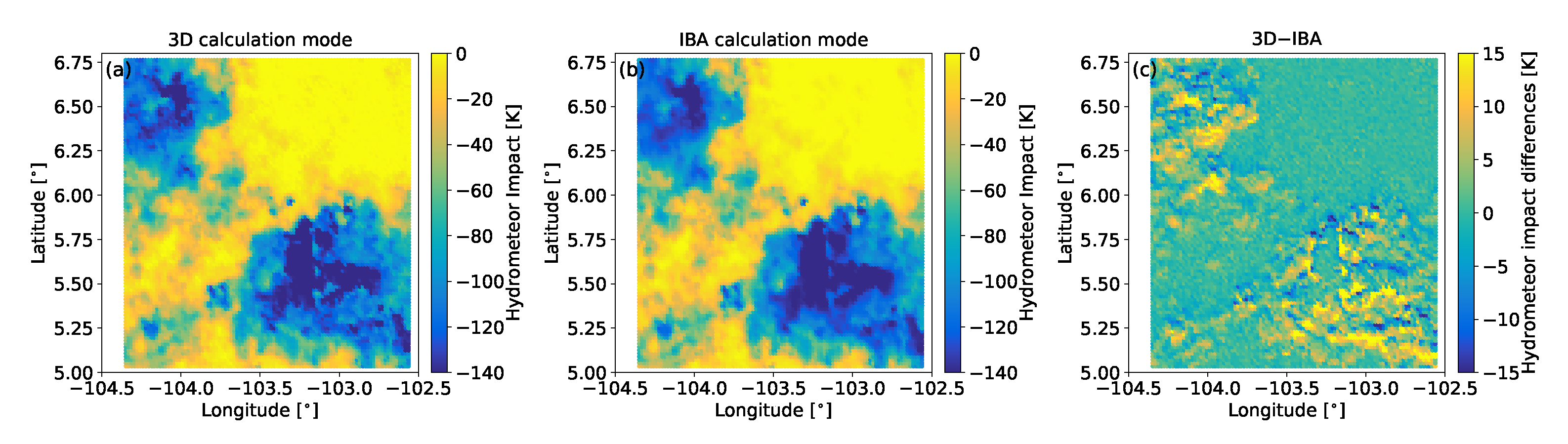
Figure 4.
Correlation of the hydrometeor impact () between IBA and 3D calculation modes for slant view in the tropics: (a) at 186.3 GHz with a footprint size of 6 km, (b) at 668 GHz with a footprint size of 6 km, (c) at 186.3 GHz with a footprint size of 15 km, and (d) at 186 GHz with a footprint size of 15 km. The one-to-one line (black line) and the linear fit (dark green line) are plotted for reference. The slope of linear regression line (a) and the coefficient of determination () are highlighted. The errors correspond to the two-standard deviation (2) of the Monte Carlo (MC) simulation; i.e., MC noise.

Figure 5.
Probability density function and whisker plot of the horizontal photon transport effect () for slant view in the tropics: (a) at 186.3 GHz with a footprint size of 6 km, (b) at 668 GHz with a footprint size of 6 km, (c) at 186.3 GHz with a footprint size of 15 km, and (d) at 186 GHz with a footprint size of 15 km. The zero difference line is marked by a black line. Boxes correspond to the interquantile range, while the crosses denote the outliers. The size of the sample (n), the mean, and the root mean square error (RMSE) of the HPT effect are highlighted.
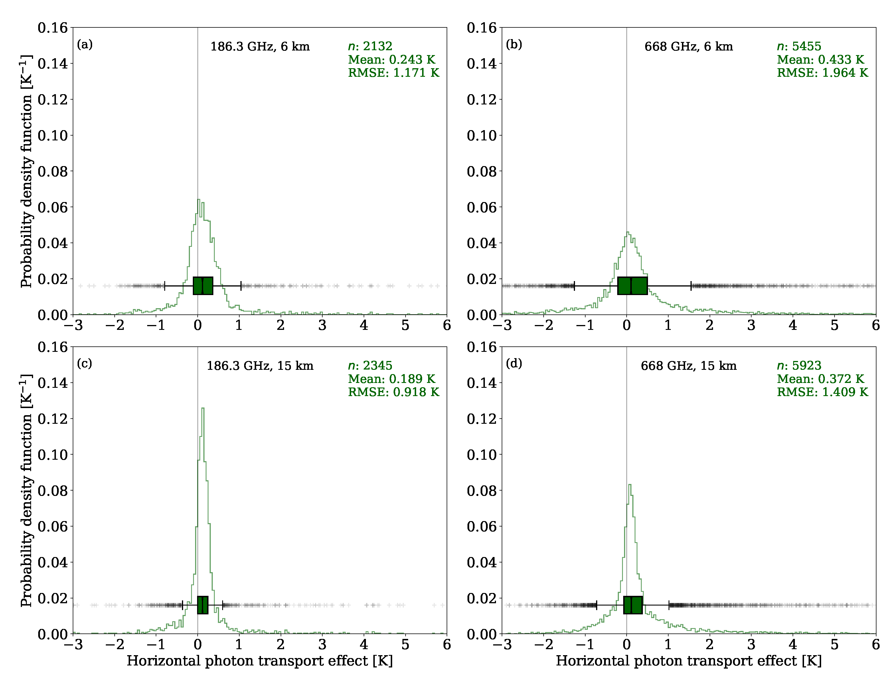
Figure 6.
The same as in Figure 4, but between IBA and both 1D calculation modes; i.e., hydrometeor number density average (HND-avg in dark blue) and hydrometeor content average (HC-avg in dark red) modes.
Figure 6.
The same as in Figure 4, but between IBA and both 1D calculation modes; i.e., hydrometeor number density average (HND-avg in dark blue) and hydrometeor content average (HC-avg in dark red) modes.

Figure 7.
The same as in Figure 5, but for the beam-filling effect () for both 1D calculation modes; i.e., HND-avg (in dark red) and HC-avg (in dark blue).
Figure 7.
The same as in Figure 5, but for the beam-filling effect () for both 1D calculation modes; i.e., HND-avg (in dark red) and HC-avg (in dark blue).

Figure 8.
The same as in Figure 7, but in the mid-latitudes.
Figure 8.
The same as in Figure 7, but in the mid-latitudes.
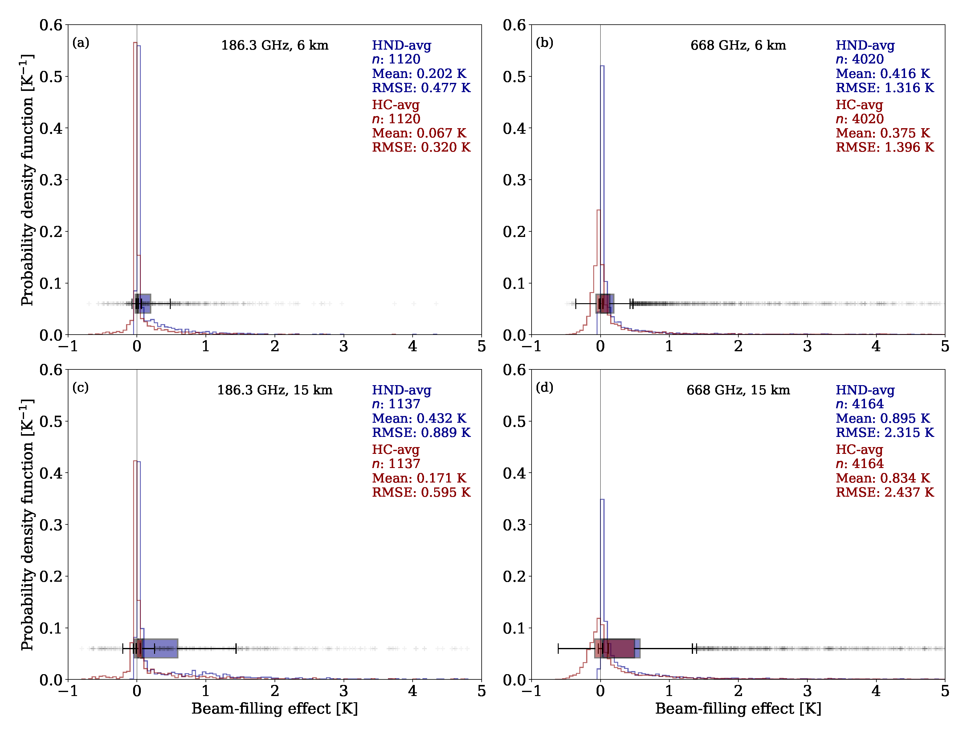

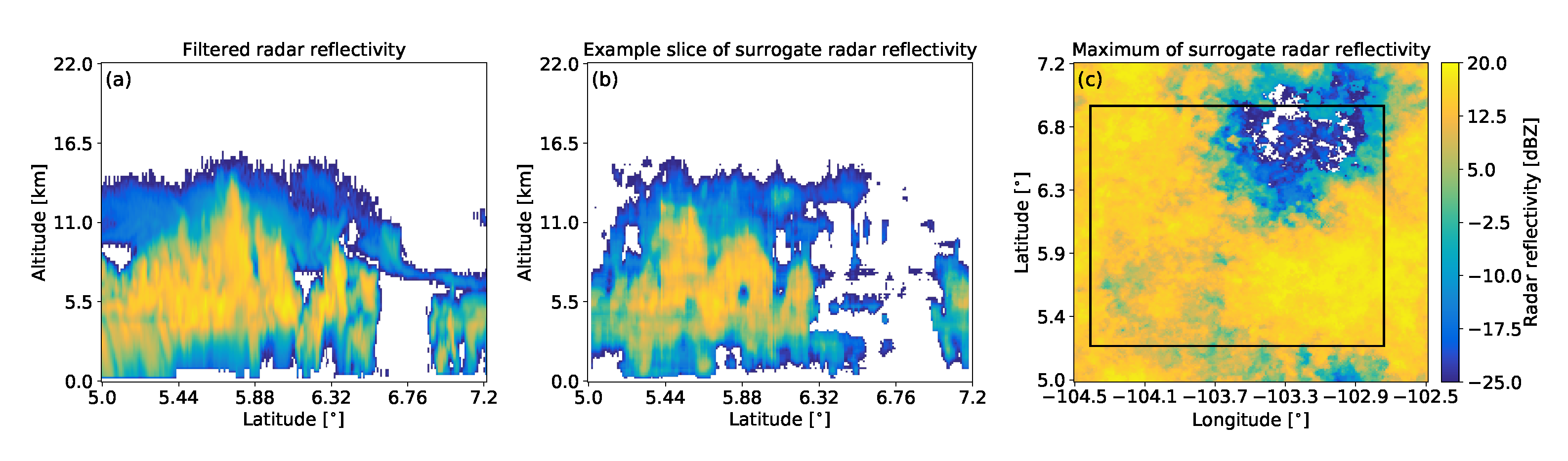
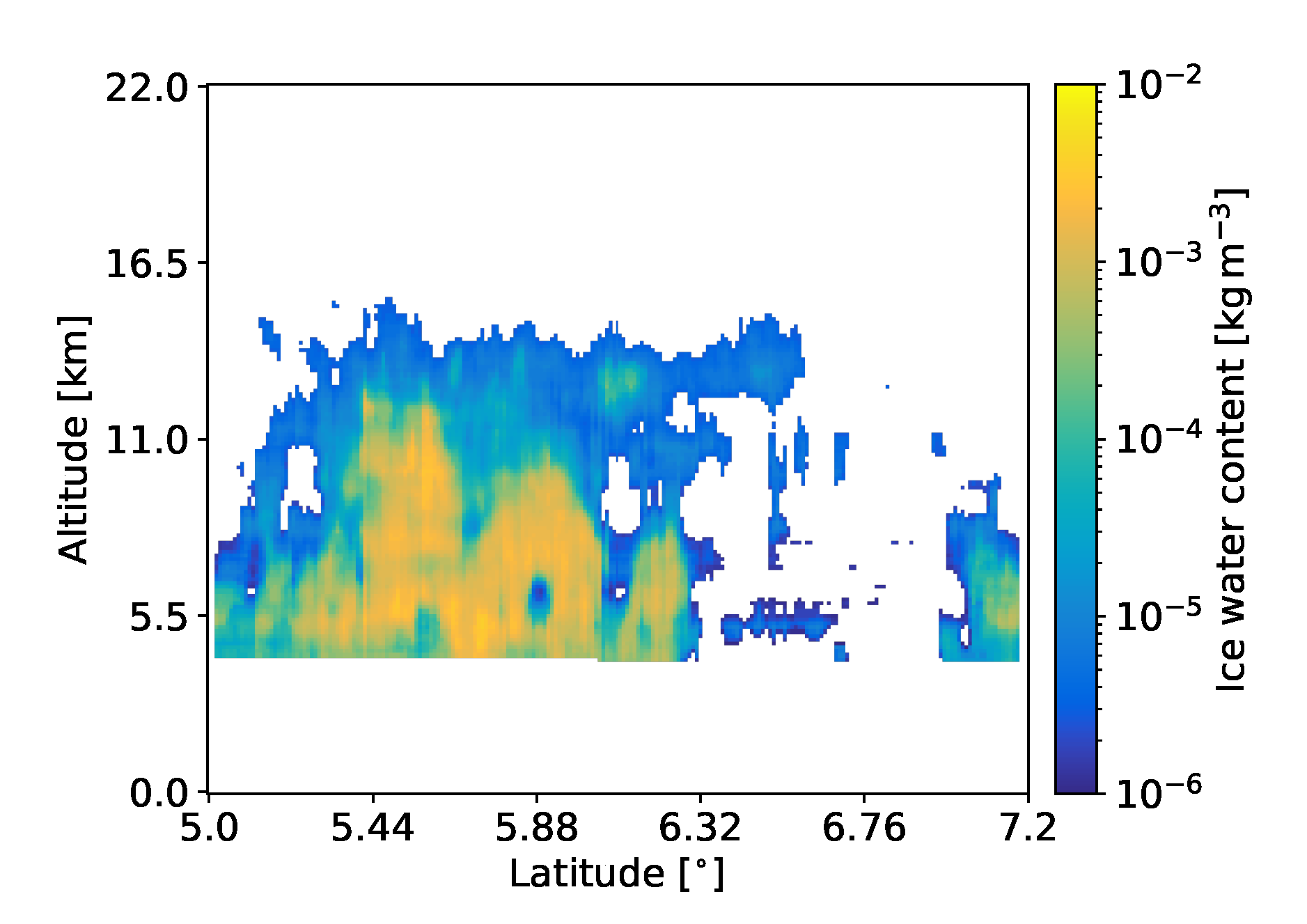
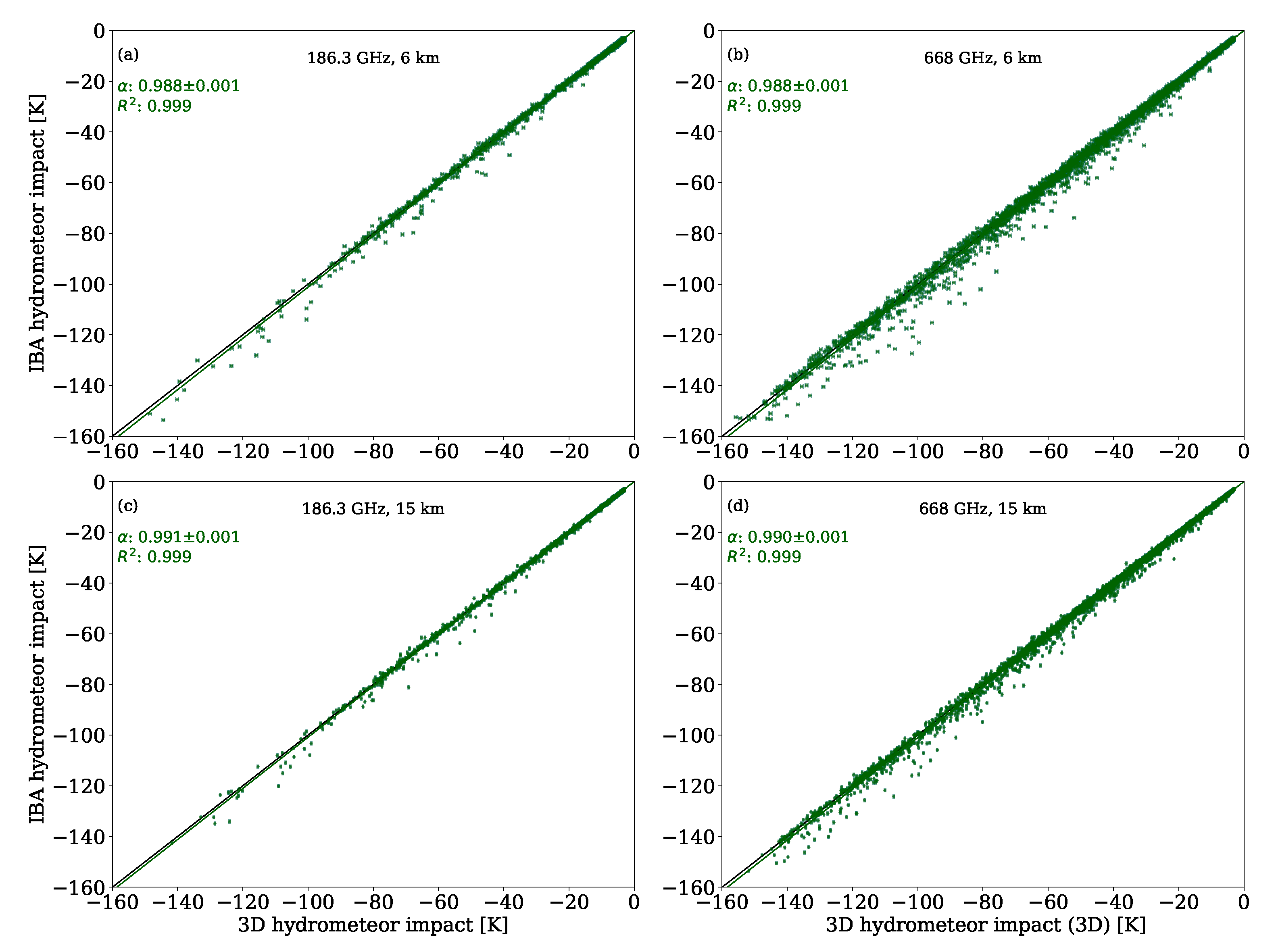
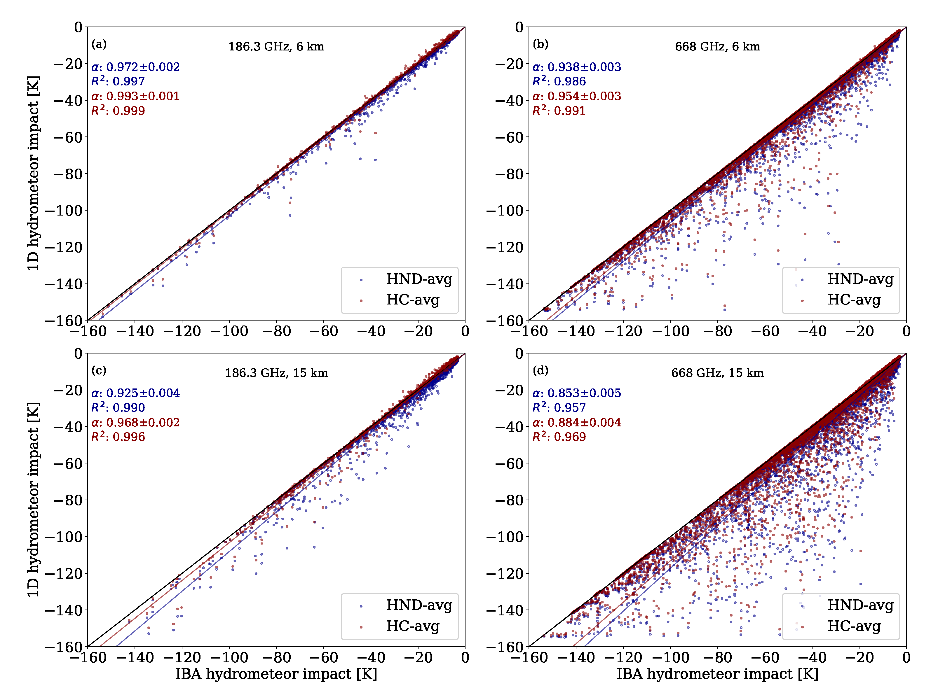
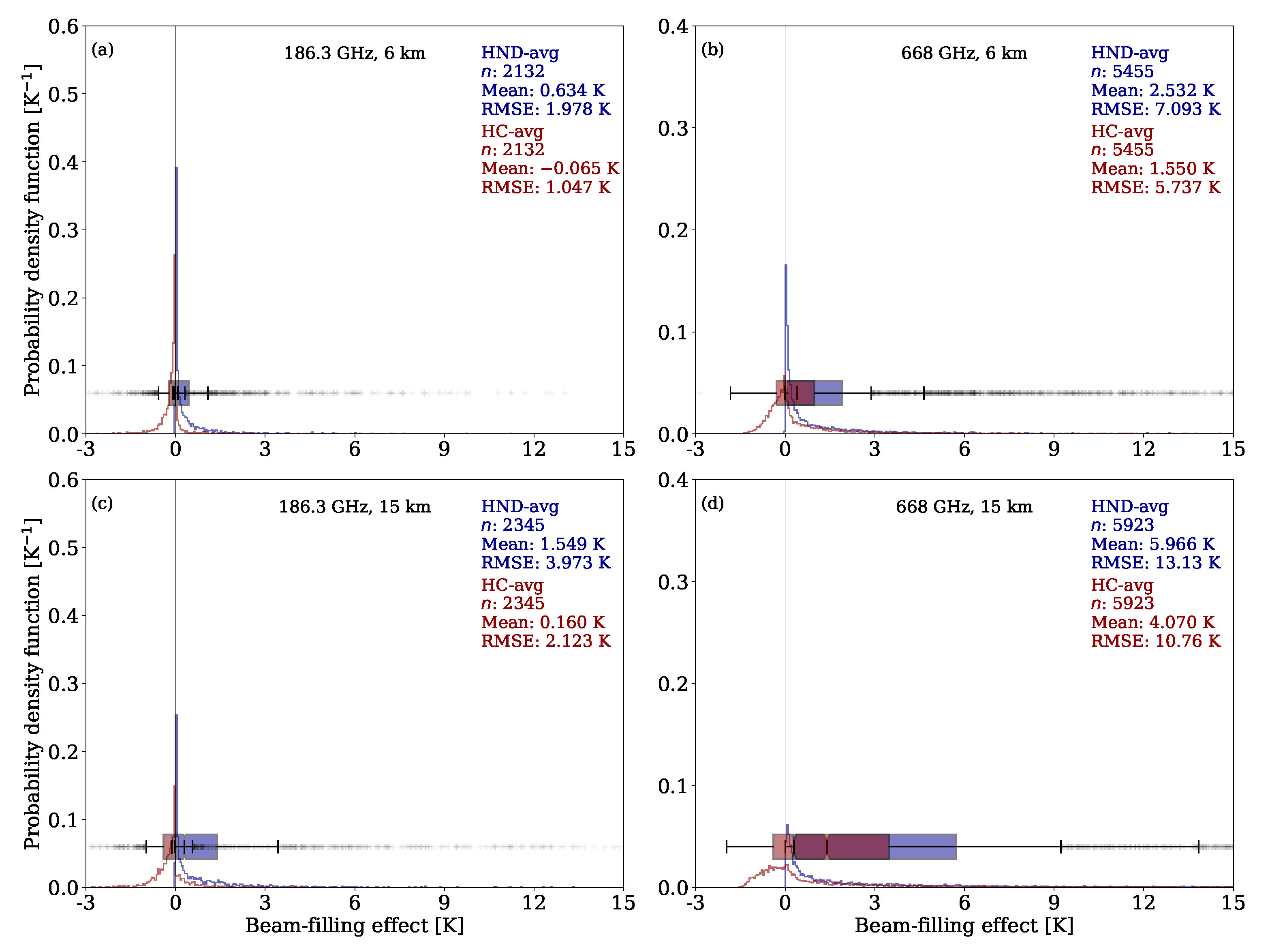
Table 1.
Statistics of the horizontal photon transport effect over both tropics and mid-latitude scenes for both slant and nadir radiative transfer simulations. Results are presented in terms of the sample size (n), mean, root mean square error (RMSE), slope of linear regression line (a), two-standard deviations of the regression slope (2), the coefficient of determination (), and the RMSE corrected by the slope of the regression line (RMSE).
| Tropics Slant | 186.3 GHz, 6 km | 668 GHz, 6 km | 186.3 GHz, 15 km | 668 GHz, 15 km |
|---|---|---|---|---|
| n | 2132 | 5455 | 2345 | 5923 |
| Mean | 0.243 | 0.433 | 0.189 | 0.372 |
| RMSE | 1.171 | 1.964 | 0.918 | 1.409 |
| 0.988 ± 0.001 | 0.988 ± 0.001 | 0.991 ± 0.001 | 0.990 ± 0.001 | |
| 0.999 | 0.999 | 0.999 | 0.999 | |
| RMSE | 1.103 | 1.868 | 0.879 | 1.317 |
| Mid-latitudes Slant | 186.3 GHz, 6 km | 668 GHz, 6 km | 186.3 GHz, 15 km | 668 GHz, 15 km |
| n | 1120 | 4020 | 1137 | 4164 |
| Mean | 0.110 | 0.046 | 0.116 | 0.045 |
| RMSE | 0.281 | 0.330 | 0.172 | 0.199 |
| 0.992 ± 0.002 | 1.000 ± 0.001 | 0.989 ± 0.001 | 1.001 ± 0.000 | |
| 0.999 | 1.000 | 1.000 | 1.000 | |
| RMSE | 0.274 | 0.329 | 0.152 | 0.199 |
| Tropics Nadir | 186.3 GHz, 6 km | 668 GHz, 6 km | 186.3 GHz, 15 km | 668 GHz, 15 km |
| n | 2072 | 5426 | 2236 | 5904 |
| Mean | 0.138 | 0.226 | 0.130 | 0.213 |
| RMSE | 0.458 | 0.676 | 0.240 | 0.447 |
| 0.999 ± 0.001 | 0.995 ± 0.000 | 0.998 ± 0.000 | 0.995 ± 0.000 | |
| 1.000 | 1.000 | 1.000 | 1.000 | |
| RMSE | 0.457 | 0.640 | 0.235 | 0.398 |
| Mid-latitudes Nadir | 186.3 GHz, 6 km | 668 GHz, 6 km | 186.3 GHz, 15 km | 668 GHz, 15 km |
| n | 1047 | 4209 | 1049 | 4395 |
| Mean | 0.139 | 0.116 | 0.148 | 0.115 |
| RMSE | 0.288 | 0.271 | 0.207 | 0.166 |
| 0.985 ± 0.002 | 0.996 ± 0.001 | 0.981 ± 0.002 | 0.996 ± 0.000 | |
| 0.999 | 1.000 | 0.999 | 1.000 | |
| RMSE | 0.267 | 0.264 | 0.169 | 0.153 |
Table 2.
The same as in Table 1, but in terms of the beam filling effect (). Results are presented for both HND-avg (hydrometeor number density average) and HC-avg (hydrometeor content average) calculation modes denoted as HND and HC within the table, respectively.
Table 2.
The same as in Table 1, but in terms of the beam filling effect (). Results are presented for both HND-avg (hydrometeor number density average) and HC-avg (hydrometeor content average) calculation modes denoted as HND and HC within the table, respectively.
| Tropics Slant | 186.3 GHz, 6 km | 668 GHz, 6 km | 186.3 GHz, 15 km | 668 GHz, 15 km | ||||
|---|---|---|---|---|---|---|---|---|
| HND | HC | HND | HC | HND | HC | HND | HC | |
| n | 2132 | 2132 | 5455 | 5455 | 2345 | 2345 | 5923 | 5923 |
| Mean | 0.634 | −0.065 | 2.532 | 1.550 | 1.549 | 0.160 | 5.966 | 4.070 |
| RMSE | 1.978 | 1.047 | 7.093 | 5.737 | 3.973 | 2.123 | 13.13 | 10.76 |
| 0.972 ± 0.001 | 0.993 ± 0.001 | 0.938 ± 0.001 | 0.954 ± 0.001 | 0.925 ± 0.002 | 0.968 ± 0.001 | 0.853 ± 0.002 | 0.884 ± 0.002 | |
| 0.997 | 0.999 | 0.986 | 0.991 | 0.990 | 0.996 | 0.957 | 0.969 | |
| RMSE | 1.723 | 1.020 | 6.185 | 5.137 | 3.056 | 1.862 | 10.17 | 8.666 |
| Mid-latitudes Slant | 186.3 GHz, 6 km | 668 GHz, 6 km | 186.3 GHz, 15 km | 668 GHz, 15 km | ||||
| HND | HC | HND | HC | HND | HC | HND | HC | |
| n | 1120 | 1120 | 4020 | 4020 | 1137 | 1137 | 4164 | 4164 |
| Mean | 0.202 | 0.067 | 0.416 | 0.375 | 0.432 | 0.171 | 0.895 | 0.834 |
| RMSE | 0.477 | 0.320 | 1.316 | 1.396 | 0.889 | 0.595 | 2.315 | 2.437 |
| 0.970 ± 0.001 | 0.986 ± 0.001 | 0.975 ± 0.001 | 0.976 ± 0.001 | 0.933 ± 0.003 | 0.967 ± 0.002 | 0.947 ± 0.002 | 0.947 ± 0.002 | |
| 0.998 | 0.999 | 0.996 | 0.995 | 0.992 | 0.995 | 0.987 | 0.985 | |
| RMSE | 0.395 | 0.296 | 1.226 | 1.314 | 0.704 | 0.534 | 2.080 | 2.217 |
| Tropics Nadir | 186.3 GHz, 6 km | 668 GHz, 6 km | 186.3 GHz, 15 km | 668 GHz, 15 km | ||||
| HND | HC | HND | HC | HND | HC | HND | HC | |
| n | 2072 | 2072 | 5462 | 5462 | 2236 | 2236 | 5904 | 5904 |
| Mean | 0.513 | 2.162 | 1.417 | 1.144 | 0.067 | 4.911 | 3.416 | |
| RMSE | 1.642 | 0.972 | 6.244 | 5.182 | 3.111 | 1.821 | 11.32 | 9.352 |
| 0.970 ± 0.001 | 0.990 ± 0.001 | 0.936 ± 0.001 | 0.950 ± 0.001 | 0.930 ± 0.002 | 0.969 ± 0.001 | 0.856 ± 0.002 | 0.885 ± 0.002 | |
| 0.998 | 0.999 | 0.987 | 0.999 | 0.992 | 0.996 | 0.959 | 0.970 | |
| RMSE | 1.382 | 0.918 | 5.375 | 4.571 | 2.379 | 1.611 | 8.768 | 7.51 |
| Mid-latitude Nadir | 186.3 GHz, 6 km | 668 GHz, 6 km | 186.3 GHz, 15 km | 668 GHz, 15 km | ||||
| HND | HC | HND | HC | HND | HC | HND | HC | |
| n | 1047 | 1047 | 4209 | 4209 | 1049 | 1049 | 4395 | 4395 |
| Mean | 0.115 | 0.057 | 0.333 | 0.341 | 0.239 | 0.128 | 0.669 | 0.691 |
| RMSE | 0.298 | 0.235 | 1.082 | 1.178 | 0.533 | 0.414 | 1.804 | 1.956 |
| 0.980 ± 0.001 | 0.988 ± 0.001 | 0.974 ± 0.001 | 0.972 ± 0.001 | 0.957 ± 0.002 | 0.973 ± 0.002 | 0.948 ± 0.002 | 0.944 ± 0.002 | |
| 0.999 | 0.999 | 0.996 | 0.995 | 0.995 | 0997 | 0.988 | 0.986 | |
| RMSE | 0.259 | 0.218 | 0.997 | 1.089 | 0.447 | 0.373 | 1.611 | 1.752 |
Table 3.
The same as in Table 2, but in terms of the combined beam-filling and horizontal photon transport effect; i.e., the total 3D effects ().
Table 3.
The same as in Table 2, but in terms of the combined beam-filling and horizontal photon transport effect; i.e., the total 3D effects ().
| Tropics Slant | 186.3 GHz, 6 km | 668 GHz, 6 km | 186.3 GHz, 15 km | 668 GHz, 15 km | ||||
|---|---|---|---|---|---|---|---|---|
| HND | HC | HND | HC | HND | HC | HND | HC | |
| n | 2132 | 2132 | 5455 | 5455 | 2345 | 2345 | 5923 | 5923 |
| Mean | 0.877 | 0.178 | 2.965 | 1.983 | 1.738 | 0.349 | 6.337 | 4.442 |
| RMSE | 2.607 | 1.721 | 8.164 | 6.841 | 4.425 | 2.612 | 13.88 | 11.53 |
| 0.960 ± 0.001 | 0.981 ± 0.001 | 0.926 ± 0.002 | 0.941 ± 0.002 | 0.916 ± 0.002 | 0.960 ± 0.001 | 0.843 ± 0.002 | 0.873 ± 0.002 | |
| 0.995 | 0.998 | 0.982 | 0.987 | 0.988 | 0.995 | 0.952 | 0.965 | |
| RMSE | 2.215 | 1.601 | 7.025 | 6.031 | 3.401 | 2.264 | 10.65 | 9.185 |
| Mid-latitudes Slant | 186.3 GHz, 6 km | 668 GHz, 6 km | 186.3 GHz, 15 km | 668 GHz, 15 km | ||||
| HND | HC | HND | HC | HND | HC | HND | HC | |
| n | 1120 | 1120 | 4020 | 4020 | 1137 | 1137 | 4164 | 4164 |
| Mean | 0.312 | 0.178 | 0.462 | 0.421 | 0.549 | 0.288 | 0.940 | 0.879 |
| RMSE | 0.572 | 0.428 | 1.445 | 1.521 | 0.944 | 0.641 | 2.408 | 2.529 |
| 0.962 ± 0.002 | 0.978 ± 0.001 | 0.976 ± 0.001 | 0.976 ± 0.001 | 0.924 ± 0.003 | 0.956 ± 0.002 | 0.947 ± 0.002 | 0.947 ± 0.002 | |
| 0.997 | 0.998 | 0.995 | 0.994 | 0.991 | 0.995 | 0.986 | 0.984 | |
| RMSE | 0.467 | 0.385 | 1.365 | 1.447 | 0.710 | 0.541 | 2.185 | 2.319 |
| Tropics Nadir | 186.3 GHz, 6 km | 668 GHz, 6 km | 186.3 GHz, 15 km | 668 GHz, 15 km | ||||
| HND | HC | HND | HC | HND | HC | HND | HC | |
| n | 2072 | 2072 | 5462 | 5462 | 2236 | 2236 | 5904 | 5904 |
| Mean | 0.651 | 0.090 | 2.389 | 1.644 | 1.273 | 0.196 | 5.123 | 3.628 |
| RMSE | 1.751 | 1.021 | 6.625 | 5.549 | 3.183 | 1.841 | 11.62 | 9.652 |
| 0.969 ± 0.001 | 0.989 ± 0.001 | 0.931 ± 0.002 | 0.945 ± 0.002 | 0.929 ± 0.002 | 0.968 ± 0.001 | 0.851 ± 0.002 | 0.880 ± 0.002 | |
| 0.997 | 0.999 | 0.985 | 0.989 | 0.992 | 0.996 | 0.957 | 0.968 | |
| RMSE | 1.489 | 0.969 | 5.668 | 4.855 | 2.429 | 1.606 | 8.959 | 7.706 |
| Mid-latitude Nadir | 186.3 GHz, 6 km | 668 GHz, 6 km | 186.3 GHz, 15 km | 668 GHz, 15 km | ||||
| HND | HC | HND | HC | HND | HC | HND | HC | |
| n | 1047 | 1047 | 4209 | 4209 | 1049 | 1049 | 4395 | 4395 |
| Mean | 0.254 | 0.196 | 0.449 | 0.457 | 0.386 | 0.275 | 0.784 | 0.806 |
| RMSE | 0.434 | 0.386 | 1.167 | 1.258 | 0.591 | 0.481 | 1.866 | 2.055 |
| 0.965 ± 0.001 | 0.973 ± 0.001 | 0.970 ± 0.001 | 0.968 ± 0.001 | 0.940 ± 0.002 | 0.955 ± 0.002 | 0.943 ± 0.002 | 0.940 ± 0.002 | |
| 0.997 | 0.998 | 0.995 | 0.995 | 0.995 | 0996 | 0.988 | 0.985 | |
| RMSE | 0.351 | 0.332 | 1.061 | 1.149 | 0.429 | 0.379 | 1.646 | 1.784 |
© 2020 by the authors. Licensee MDPI, Basel, Switzerland. This article is an open access article distributed under the terms and conditions of the Creative Commons Attribution (CC BY) license (http://creativecommons.org/licenses/by/4.0/).
Share and Cite
MDPI and ACS Style
Barlakas, V.; Eriksson, P. Three Dimensional Radiative Effects in Passive Millimeter/Sub-Millimeter All-sky Observations. Remote Sens. 2020, 12, 531. https://doi.org/10.3390/rs12030531
AMA Style
Barlakas V, Eriksson P. Three Dimensional Radiative Effects in Passive Millimeter/Sub-Millimeter All-sky Observations. Remote Sensing. 2020; 12(3):531. https://doi.org/10.3390/rs12030531
Chicago/Turabian StyleBarlakas, Vasileios, and Patrick Eriksson. 2020. "Three Dimensional Radiative Effects in Passive Millimeter/Sub-Millimeter All-sky Observations" Remote Sensing 12, no. 3: 531. https://doi.org/10.3390/rs12030531
Note that from the first issue of 2016, this journal uses article numbers instead of page numbers. See further details here.