How Well Do Deep Learning-Based Methods for Land Cover Classification and Object Detection Perform on High Resolution Remote Sensing Imagery?

Abstract
:
1. Introduction
- Providing a comprehensive overview on classification and object detection approaches of land cover using high resolution remote sensing imagery;
- Through two real application case studies, evaluating the performances of existing deep-learning-based approaches on high resolution images for land cover classification and object detection;
- Discussing the limitations of existing deep learning methods using high resolution remote sensing imagery and providing insights on the future trends of classification and object detection methods of land cover.
2. Overview of Land Cover Classification and Object Detection on High Resolution Remote Sensing Imagery
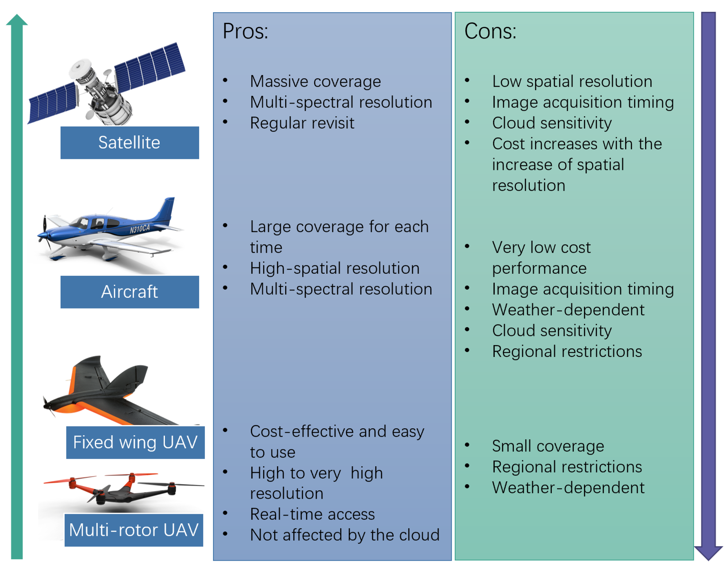
2.1. Recent Progresses in the Availability of High-Resolution Remote Sensing Imagery for Land Cover
2.2. Traditional Approaches for Land Cover Classification at Pixel Level
2.2.1. Unsupervised Classification
ISODATA
K-Means
2.2.2. Supervised Classification
CART
Random Forest (RF)
Support Vector Machine (SVM)
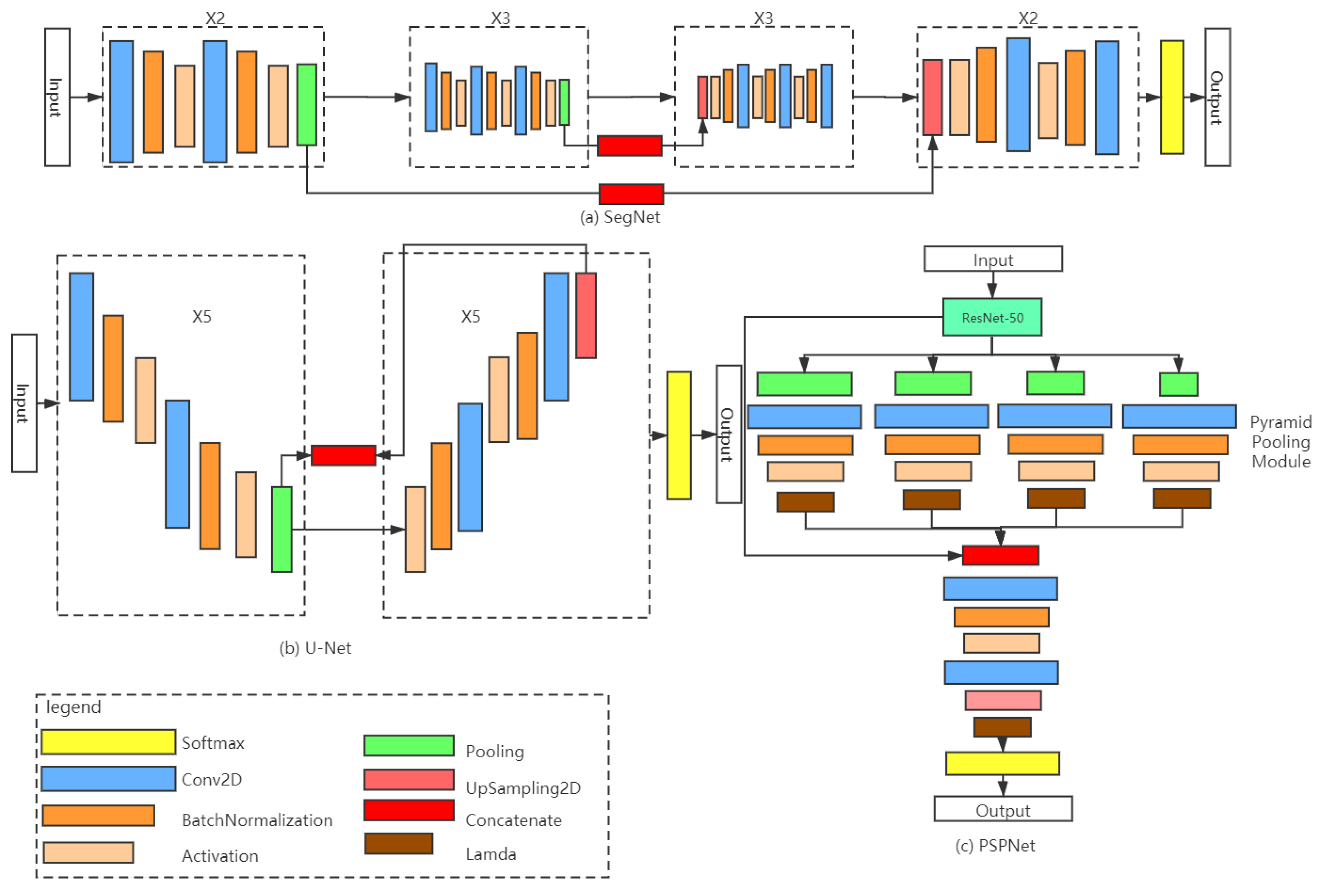
2.3. Deep Learning-Based Semantic Segmentation Classification of Land Cover at the Pixel Level
2.3.1. SegNet
2.3.2. U-Net
2.3.3. PSPNet
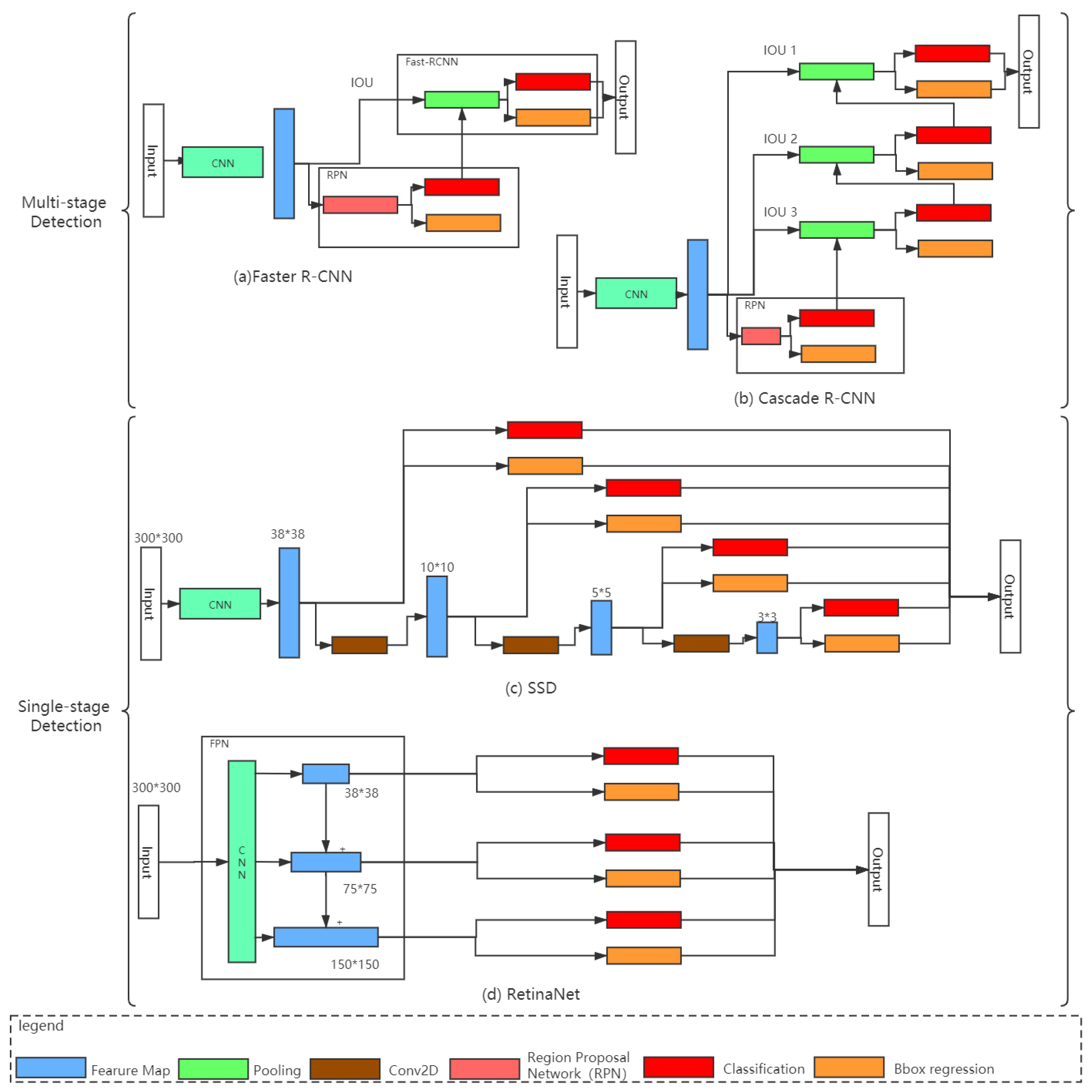
2.4. Deep Learning-Based Object Detection for Land Cover at an Object Level
2.4.1. Faster R-CNN/Cascade R-CNN
2.4.2. SSD/RetinaNet
3. Two Case Studies Using Deep Learning-Based Approaches
- Land cover classification on 5 m high resolution imagery at a pixel level. The high-quality land cover products in high spatial resolution can provide very detailed information which can be used in almost all studies on Earth’s ecosystems.
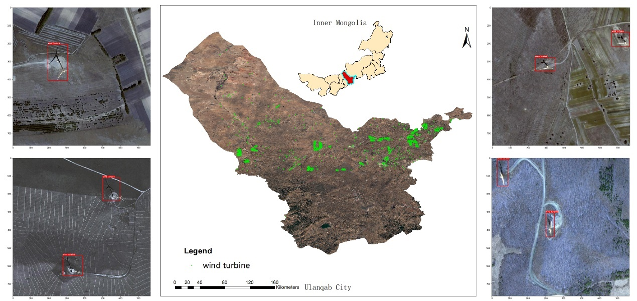
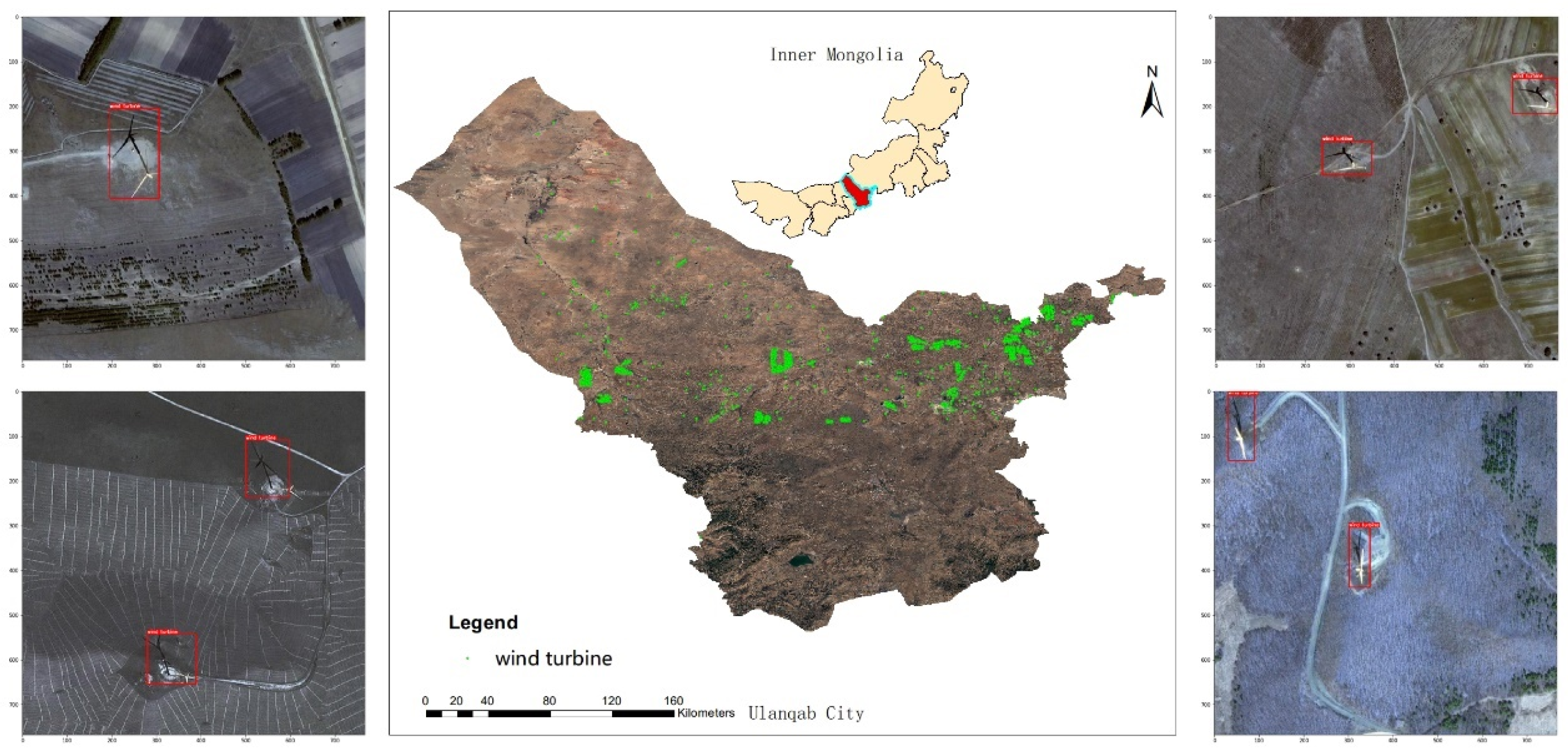
- Wind turbine quantity and location detection on Google Earth’s imagery at an object level. The accurate location information in large areas can help researchers evaluate the impact of the rapidly growing use of wind turbines on wildlife and climate changes.
3.1. Land Cover Classification Using Deep Learning Approaches at the Pixel Level
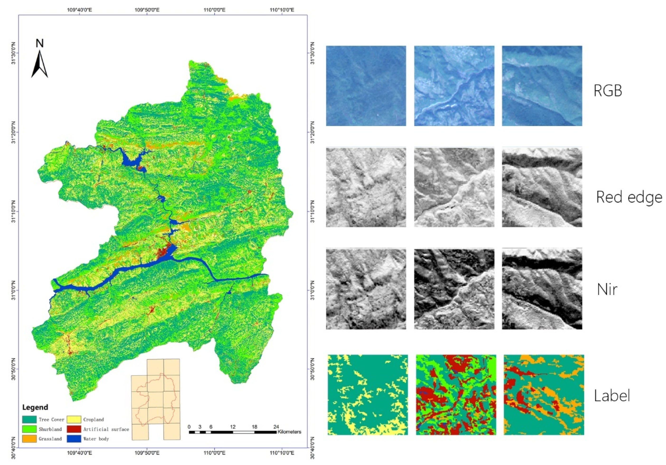
3.1.1. Study Area
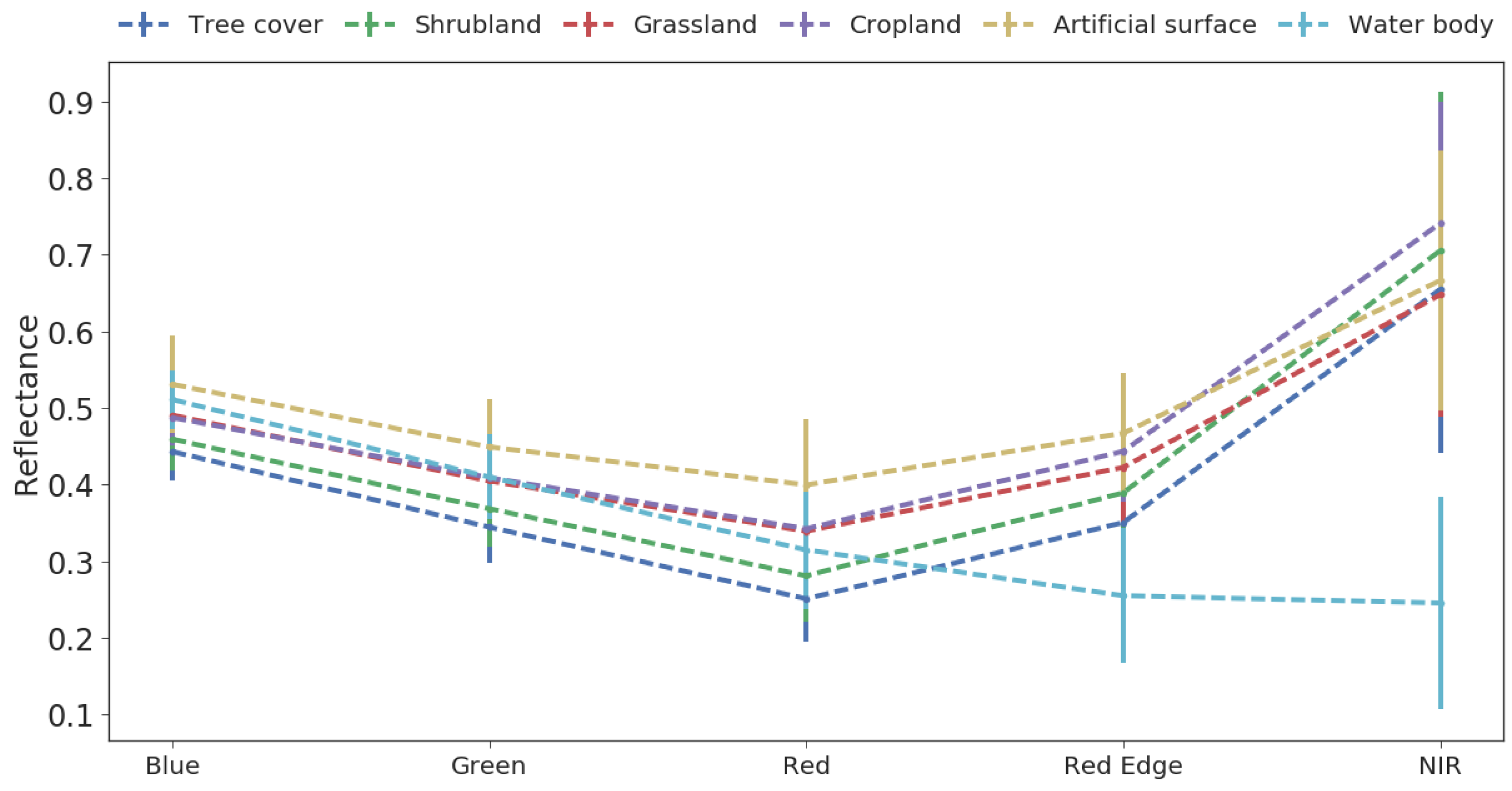
3.1.2. Data Descriptions
3.1.3. Performance Evaluation Metric
3.1.4. Experimental Evaluation
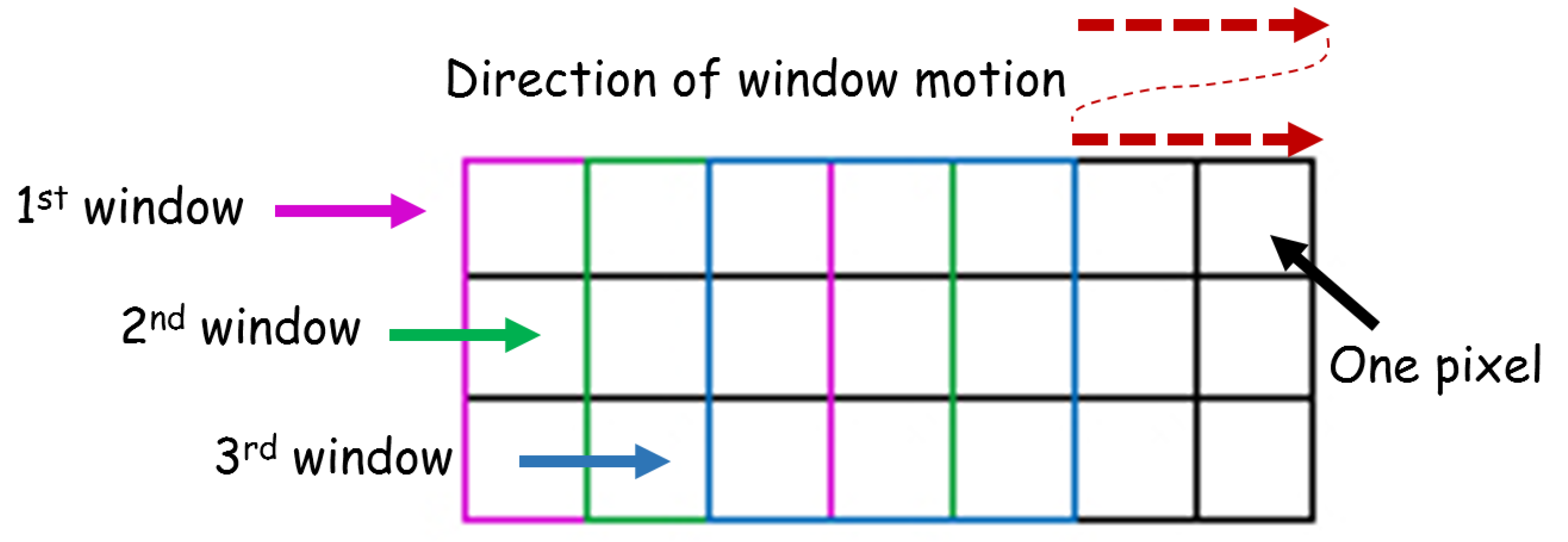
Data Preprocessing
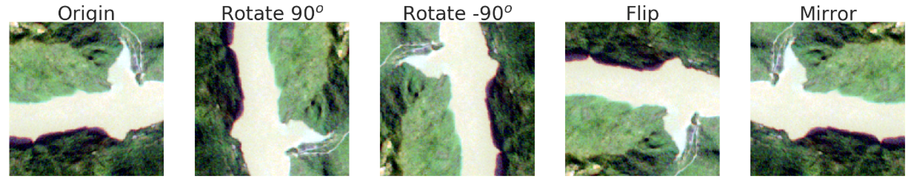
Data Augmentation
Model Training
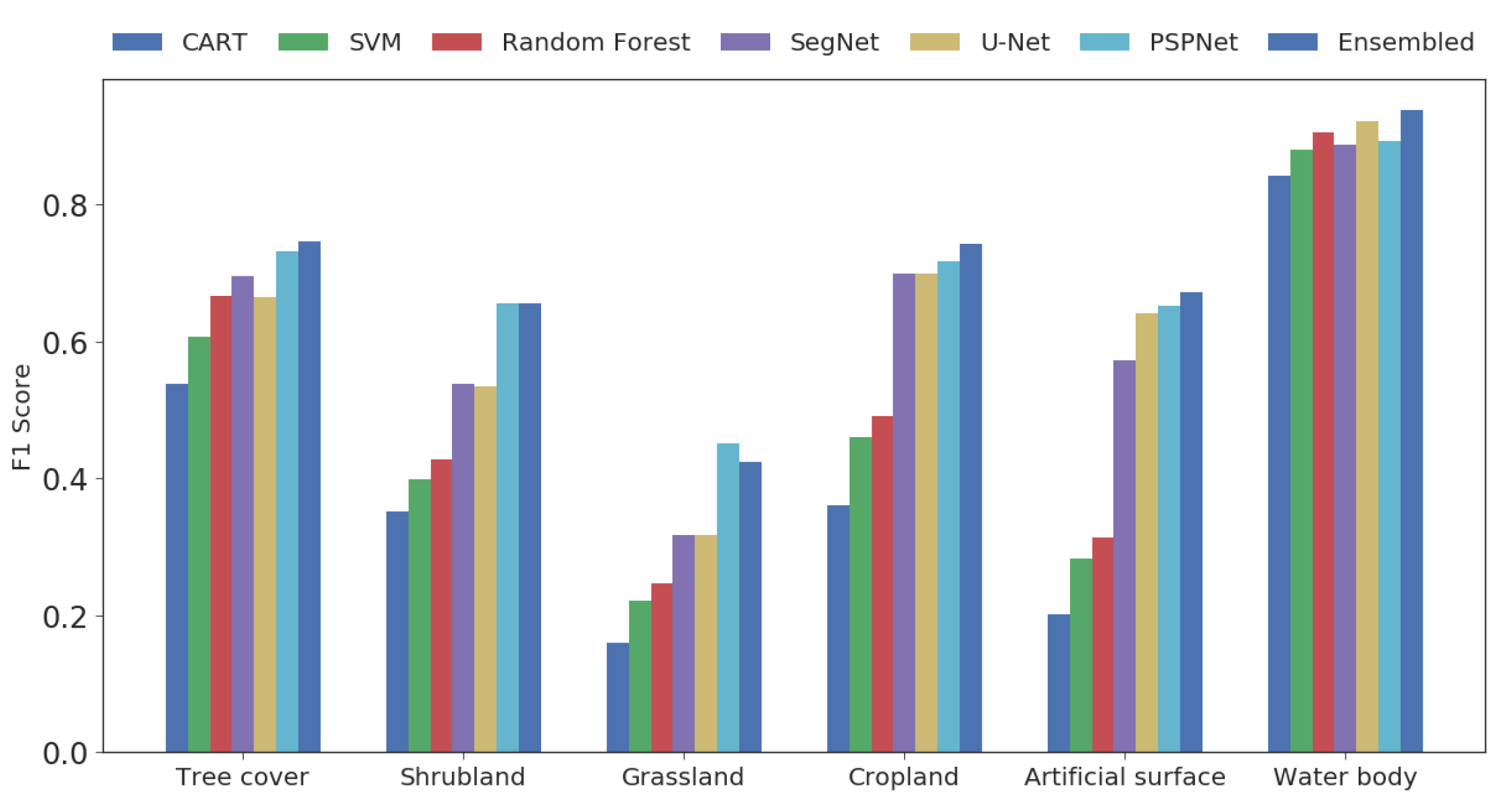
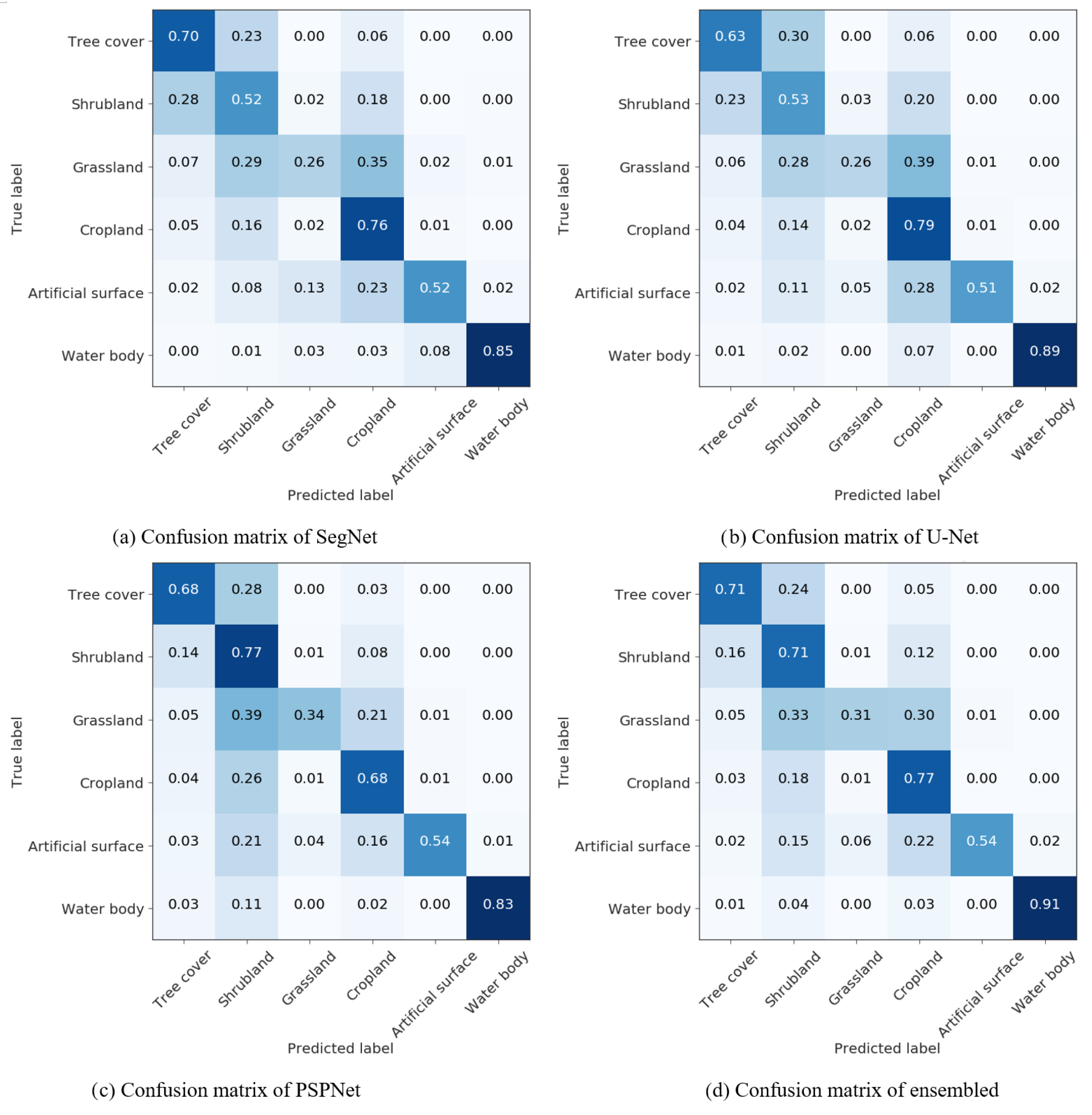
3.1.5. Experimental Results
3.2. Land Cover Object Detection Using Deep Learning Approaches at an Object Level
3.2.1. Study Area
3.2.2. Data Description
3.2.3. Performance Evaluation Metric
3.2.4. Experimental Evaluation
Model Training
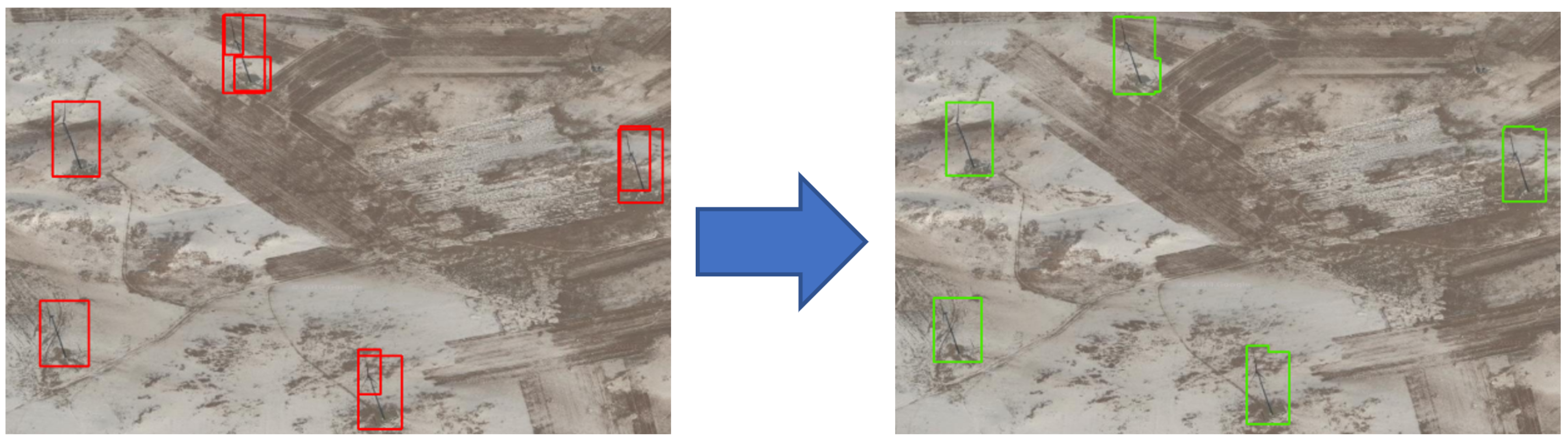
Post Processing
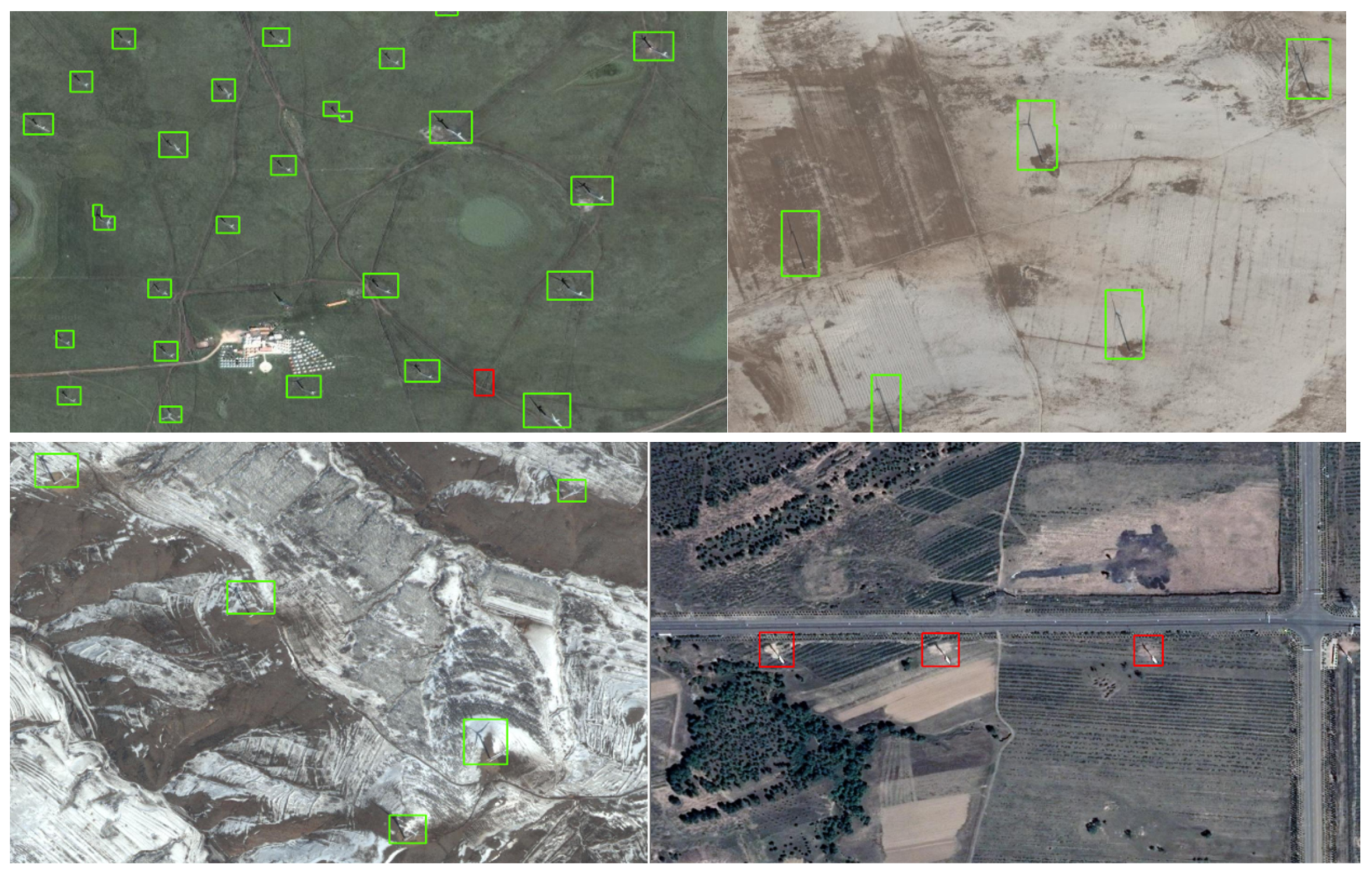
Experimental Results
4. Discussion
4.1. Land Cover Classification
4.2. Land Cover Object Detection
5. Conclusions
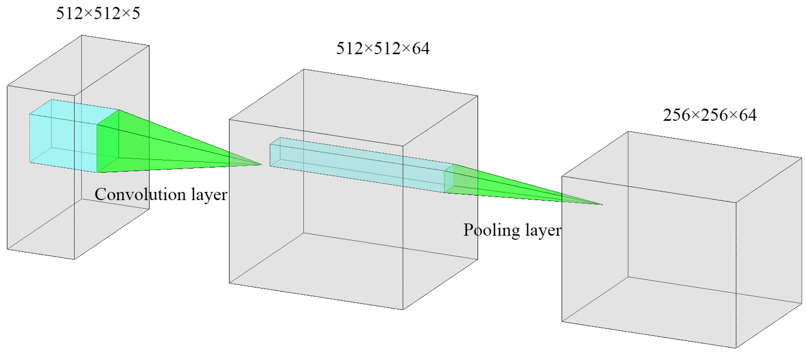
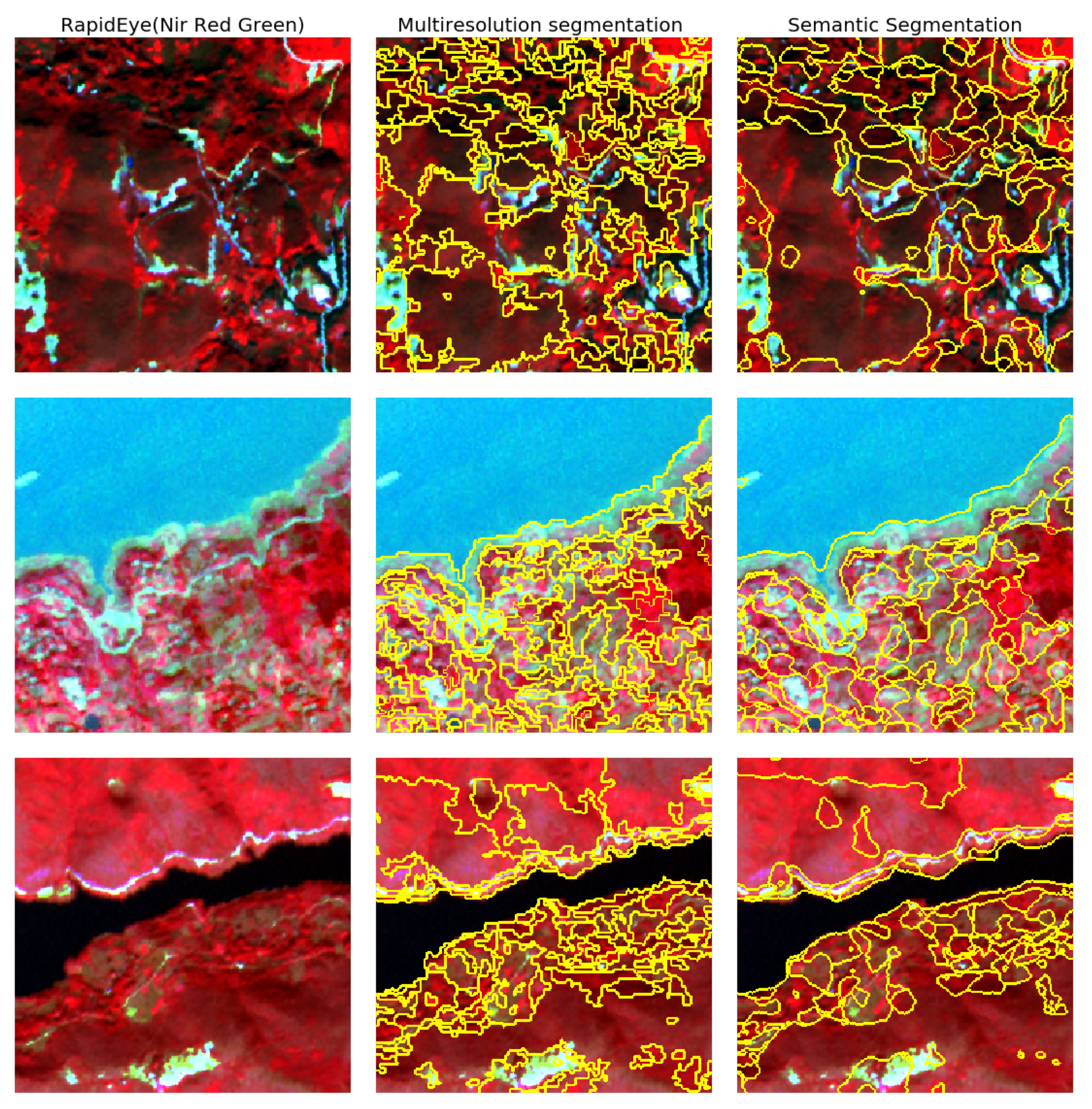
- For land cover classification, the state of the art semantic segmentation deep-learning-based methods at a pixel level performed better than the pixel-based classification methods using traditional machine learning approaches through leveraging spatial information in convolution layer. Meanwhile, from the visual aspect, the segmentation results based on the deep learning method produced a visually appealing generalised appearance of land cover better than that from one of the most widely used object-based segmentation methods.
- Considering the diversity of remote sensing data, most land cover studies on high-resolution imagery have limited training data sets, which reduces the robustness of a deep learning-based model. The deep learning-based model cannot completely replace the traditional pixel-based methods in practice.
- A satisfying evaluation result was achieved for the current state-of-the-art deep learning-based models for a real object detection task. The deep learning-based models could relieve the burden of the traditional, labour-intensive objective detection task.
Author Contributions
Funding
Acknowledgments
Conflicts of Interest
References
- Rawat, J.S.; Kumar, M. Monitoring land use/cover change using remote sensing and GIS techniques: A case study of Hawalbagh block, district Almora, Uttarakhand, India. Egypt. J. Remote Sens. Space Sci. 2015, 18, 77–84. [Google Scholar] [CrossRef] [Green Version]
- Ban, Y.; Gong, P.; Giri, C. Global land cover mapping using Earth observation satellite data: Recent progresses and challenges. ISPRS J. Photogramm. Remote Sens. 2015, 103, 1–6. [Google Scholar] [CrossRef] [Green Version]
- Feddema, J.J. The Importance of Land-Cover Change in Simulating Future Climates. Science 2005, 310, 1674–1678. [Google Scholar] [CrossRef] [Green Version]
- Duro, D.C.; Franklin, S.E.; Dubé, M.G. A comparison of pixel-based and object-based image analysis with selected machine learning algorithms for the classification of agricultural landscapes using SPOT-5 HRG imagery. Remote Sens. Environ. 2012, 118, 259–272. [Google Scholar] [CrossRef]
- Schowengerdt, R.A. CHAPTER 9—Thematic Classification. In Remote Sensing, 3rd ed.; Academic Press: Burlington, NJ, USA, 2007. [Google Scholar] [CrossRef]
- Chasmer, L.; Hopkinson, C.; Veness, T.; Quinton, W.; Baltzer, J. A decision-tree classification for low-lying complex land cover types within the zone of discontinuous permafrost. Remote Sens. Environ. 2014, 143, 73–84. [Google Scholar] [CrossRef]
- Friedl, M.A.; Brodley, C.E. Decision tree classification of land cover from remotely sensed data. Remote Sens. Environ. 1997, 61, 399–409. [Google Scholar] [CrossRef]
- Hua, L.; Zhang, X.; Chen, X.; Yin, K.; Tang, L. A Feature-Based Approach of Decision Tree Classification to Map Time Series Urban Land Use and Land Cover with Landsat 5 TM and Landsat 8 OLI in a Coastal City, China. Int. J. Geo-Inf. 2017, 6, 331. [Google Scholar] [CrossRef] [Green Version]
- Melgani, F.; Bruzzone, L. Classification of hyperspectral remote sensing images with support vector machines. IEEE Trans. Geosci. Remote Sens. 2004, 42, 1778–1790. [Google Scholar] [CrossRef] [Green Version]
- Benz, U.C.; Hofmann, P.; Willhauck, G.; Lingenfelder, I.; Heynen, M. Multi-resolution, object-oriented fuzzy analysis of remote sensing data for GIS-ready information. ISPRS J. Photogramm. Remote Sens. 2004, 58, 239–258. [Google Scholar] [CrossRef]
- Munoz-Mari, J.; Bovolo, F.; Gomez-Chova, L.; Bruzzone, L.; Camp-Valls, G. Semisupervised One-Class Support Vector Machines for Classification of Remote Sensing Data. IEEE Trans. Geosci. Remote Sens. 2010, 48, 3188–3197. [Google Scholar] [CrossRef] [Green Version]
- Beijma, S.V.; Comber, A.; Lamb, A. Random forest classification of salt marsh vegetation habitats using quad-polarimetric airborne SAR, elevation and optical RS data. Remote Sens. Environ. 2014, 149, 118–129. [Google Scholar] [CrossRef]
- Khatami, R.; Mountrakis, G.; Stehman, S.V. A meta-analysis of remote sensing research on supervised pixel-based land-cover image classification processes: General guidelines for practitioners and future research. Remote Sens. Environ. 2016, 177, 89–100. [Google Scholar] [CrossRef] [Green Version]
- Dean, A.M.; Smith, G.M. An evaluation of per-parcel land cover mapping using maximum likelihood class probabilities. Int. J. Remote Sens. 2003, 24, 2905–2920. [Google Scholar] [CrossRef]
- Blaschke, T.; Lang, S.; Lorup, E.; Strobl, J.; Zeil, P. Object-Oriented Image Processing in an Integrated GIS/Remote Sensing Environment and Perspectives for Environmental Applications. Environ. Inf. Plan. Politics Public 2000, 2, 555–570. [Google Scholar]
- Blaschke, T. Object based image analysis for remote sensing. ISPRS J. Photogramm. Remote Sens. 2010, 65, 2–16. [Google Scholar] [CrossRef] [Green Version]
- Weih, R.C.; Riggan, N.D. Object-Based Classification vs. Pixel-Based Classification: Comparitive Importance of Multi-Resolution Imagery. Int. Arch. Photogramm. Remote Sens. Spat. Inf. Sci. 2010, 38, C7. [Google Scholar]
- Whiteside, T.G.; Boggs, G.S.; Maier, S.W. Comparing object-based and pixel-based classifications for mapping savannas. Int. J. Appl. Earth Obs. Geoinf. 2011, 13, 884–893. [Google Scholar] [CrossRef]
- Zhang, L.; Li, X.; Yuan, Q.; Liu, Y. Object-based approach to national land cover mapping using HJ satellite imagery. J. Appl. Remote Sens. 2014, 8, 083686. [Google Scholar] [CrossRef]
- Ding, X.Y. The Application of eCognition in Land Use Projects. Geomat. Spat. Inf. Technol. 2005, 28, 116–120. [Google Scholar]
- Blaschke, T.; Burnett, C.; Pekkarinen, A. Image segmentation methods for object-based analysis and classification. In Remote Sensing Image Analysis: Including the Spatial Domain; Springer: Dordrecht, The Netherlands, 2004; pp. 211–236. [Google Scholar]
- Burnett, C.; Blaschke, T. A multi-scale segmentation/object relationship modelling methodology for landscape analysis. Ecol. Model. 2003, 168, 233–249. [Google Scholar] [CrossRef]
- Adams, R.; Bischof, L. Seeded Region Growing. IEEE Trans. Pattern Anal. Mach. Intell. 1994, 16, 641–647. [Google Scholar] [CrossRef] [Green Version]
- Tilton, J.C. Image segmentation by region growing and spectral clustering with a natural convergence criterion. In Proceedings of the IGARSS’98. Sensing and Managing the Environment. 1998 IEEE International Geoscience and Remote Sensing. Symposium Proceedings. (Cat. No.98CH36174), Seattle, WA, USA, 6–10 July 1998; Volume 4, pp. 1766–1768. [Google Scholar]
- Baatz, M.; Schäpe, A. An optimization approach for high quality multi-scale image segmentation. In Proceedings of the Beiträge zum AGIT-Symposium, Salzburg, Austria, July 2000; pp. 12–23. [Google Scholar]
- Roerdink, J.B.; Meijster, A. The watershed transform: Definitions, algorithms and parallelization strategies. Fundam. Inform. 2000, 41, 187–228. [Google Scholar] [CrossRef] [Green Version]
- Audebert, N.; Boulch, A.; Randrianarivo, H.; Le Saux, B.; Ferecatu, M.; Lefevre, S.; Marlet, R. Deep learning for urban remote sensing. In Proceedings of the 2017 Joint Urban Remote Sensing Event (JURSE), Dubai, UAE, 6–8 March 2017; IEEE: Dubai, UAE, 2017; pp. 1–4. [Google Scholar]
- Contreras, D.; Blaschke, T.; Tiede, D.; Jilge, M. Monitoring recovery after earthquakes through the integration of remote sensing, GIS, and ground observations: The case of L’Aquila (Italy). Cartogr. Geogr. Inf. Sci. 2016, 43, 115–133. [Google Scholar] [CrossRef]
- Nebiker, S.; Lack, N.; Deuber, M. Building Change Detection from Historical Aerial Photographs Using Dense Image Matching and Object-Based Image Analysis. Remote Sens. 2014, 6, 8310–8336. [Google Scholar] [CrossRef] [Green Version]
- Li, X.; Myint, S.W.; Zhang, Y.; Galletti, C.; Zhang, X.; Turner, B.L. Object-based land-cover classification for metropolitan Phoenix, Arizona, using aerial photography. Int. J. Appl. Earth Obs. Geoinf. 2014, 33, 321–330. [Google Scholar] [CrossRef]
- He, K.; Zhang, X.; Ren, S.; Sun, J. Deep residual learning for image recognition. In Proceedings of the IEEE Conference on Computer Vision and Pattern Recognition, Las Vegas, NV, USA, 26 June–1 July 2016; pp. 770–778. [Google Scholar]
- Szegedy, C.; Ioffe, S.; Vanhoucke, V.; Alemi, A.A. Inception-v4, inception-resnet and the impact of residual connections on learning. In Proceedings of the Thirty-First AAAI Conference on Artificial Intelligence, San Francisco, CA, USA, 4–10 February 2017. [Google Scholar]
- Ren, S.; He, K.; Girshick, R.; Sun, J. Faster R-CNN: Towards Real-Time Object Detection with Region Proposal Networks. arXiv 2015, arXiv:1506.01497. [Google Scholar] [CrossRef] [Green Version]
- Redmon, J.; Divvala, S.; Girshick, R.; Farhadi, A. You only look once: Unified, real-time object detection. In Proceedings of the IEEE Conference on Computer Vision and Pattern Recognition, Las Vegas, NV, USA, 26 June–1 July 2016; pp. 779–788. [Google Scholar]
- Ronneberger, O.; Fischer, P.; Brox, T. U-Net: Convolutional Networks for Biomedical Image Segmentation. In International Conference on Medical Image Computing and Computer-Assisted Intervention; Springer: Cham, Switzerland, 2015; pp. 234–241. [Google Scholar]
- Zhao, H.; Shi, J.; Qi, X.; Wang, X.; Jia, J. Pyramid Scene Parsing Network. In Proceedings of the IEEE Conference on Computer Vision and Pattern Recognition, Las Vegas, NV, USA, 26 June–1 July 2016. [Google Scholar]
- Krizhevsky, A.; Sutskever, I.; Hinton, G.E. ImageNet classification with deep convolutional neural networks. In Proceedings of the Advances in Neural Information Processing Systems, Lake Tahoe, NV, USA, 3–6 December 2012; pp. 1097–1105. [Google Scholar]
- Audebert, N.; Saux, B.L.; Lefèvre, S. Semantic Segmentation of Earth Observation Data Using Multimodal and Multi-scale Deep Networks. arXiv 2016, arXiv:1609.06846. [Google Scholar]
- Huang, B.; Zhao, B.; Song, Y. Urban land-use mapping using a deep convolutional neural network with high spatial resolution multispectral remote sensing imagery. Remote Sens. Environ. 2018, 214, 73–86. [Google Scholar] [CrossRef]
- Kemker, R.; Salvaggio, C.; Kanan, C. Algorithms for Semantic Segmentation of Multispectral Remote Sensing Imagery using Deep Learning. ISPRS J. Photogramm. Remote Sens. 2018, 145, 60–77. [Google Scholar] [CrossRef] [Green Version]
- Zheng, C.; Wang, L. Semantic Segmentation of Remote Sensing Imagery Using Object-Based Markov Random Field Model With Regional Penalties. IEEE J. Sel. Top. Appl. Earth Obs. Remote Sens. 2015, 8, 1924–1935. [Google Scholar] [CrossRef]
- Van Etten, A. You Only Look Twice: Rapid Multi-Scale Object Detection In Satellite Imagery. arXiv 2018, arXiv:1805.09512. [Google Scholar]
- Van Etten, A. Satellite Imagery Multiscale Rapid Detection with Windowed Networks. arXiv 2018, arXiv:1809.09978. [Google Scholar]
- Congalton, R.G.; Gu, J.; Yadav, K.; Thenkabail, P.; Ozdogan, M. Global Land Cover Mapping: A Review and Uncertainty Analysis. Remote Sens. 2014, 6, 12070–12093. [Google Scholar] [CrossRef] [Green Version]
- Rogan, J.; Chen, D. Remote sensing technology for mapping and monitoring land-cover and land-use change. Prog. Plan. 2004, 61, 301–325. [Google Scholar] [CrossRef]
- Bartholome, E.; Belward, A.S. GLC2000: A new approach to global land cover mapping from Earth observation data. Int. J. Remote Sens. 2005, 26, 1959–1977. [Google Scholar] [CrossRef]
- Bontemps, S.; Defourny, P.; Bogaert, E.V.; Arino, O.; Kalogirou, V.; Perez, J.R. GLOBCOVER 2009-Products Description and Validation Report. 2011. Available online: https://epic.awi.de/id/eprint/31014/16/GLOBCOVER2009_Validation_Report_2-2.pdf (accessed on 28 April 2019).
- Hansen, M.C.; Defries, R.S.; Townshend, J.R.G.; Sohlberg, R. Global land cover classification at 1 km spatial resolution using a classification tree approach. Int. J. Remote Sens. 2000, 21, 1331–1364. [Google Scholar] [CrossRef]
- Li, W.; Ciais, P.; MacBean, N.; Peng, S.; Defourny, P.; Bontemps, S. Major forest changes and land cover transitions based on plant functional types derived from the ESA CCI Land Cover product. Int. J. Appl. Earth Obs. Geoinf. 2016, 47, 30–39. [Google Scholar] [CrossRef]
- Mora, B.; Tsendbazar, N.E.; Herold, M.; Arino, O. Global Land Cover Mapping: Current Status and Future Trends; Springer: Dordrecht, The Netherlands, 2014. [Google Scholar]
- Fritz, S.; See, L. Identifying and quantifying uncertainty and spatial disagreement in the comparison of Global Land Cover for different applications. Glob. Chang. Biol. 2008, 14, 1057–1075. [Google Scholar] [CrossRef]
- Herold, M.; Mayaux, P.; Woodcock, C.E.; Baccini, A.; Schmullius, C. Some challenges in global land cover mapping: An assessment of agreement and accuracy in existing 1 km datasets. Remote Sens. Environ. 2008, 112, 2538–2556. [Google Scholar] [CrossRef]
- Latifovic, R.; Olthof, I. Accuracy assessment using sub-pixel fractional error matrices of global land cover products derived from satellite data. Remote Sens. Environ. 2004, 90, 153–165. [Google Scholar] [CrossRef]
- Hansen, M.C.; Loveland, T.R. A review of large area monitoring of land cover change using Landsat data. Remote Sens. Environ. 2012, 122, 66–74. [Google Scholar] [CrossRef]
- Malenovskỳ, Z.; Rott, H.; Cihlar, J.; Schaepman, M.E.; García-Santos, G.; Fernandes, R.; Berger, M. Sentinels for science: Potential of Sentinel-1,-2, and-3 missions for scientific observations of ocean, cryosphere, and land. Remote Sens. Environ. 2012, 120, 91–101. [Google Scholar] [CrossRef]
- Dial, G.; Bowen, H.; Gerlach, F.; Grodecki, J.; Oleszczuk, R. IKONOS satellite, imagery, and products. Remote Sens. Environ. 2003, 88, 23–36. [Google Scholar] [CrossRef]
- Chevrel, M.; Courtois, M.; Weill, G. The SPOT satellite remote sensing mission. Photogramm. Eng. Remote Sens. 1981, 47, 1163–1171. [Google Scholar]
- Pádua, L.; Vanko, J.; Hruška, J.; Ad ao, T.; Sousa, J.J.; Peres, E.; Morais, R. UAS, sensors, and data processing in agroforestry: A review towards practical applications. Int. J. Remote Sens. 2017, 38, 2349–2391. [Google Scholar] [CrossRef]
- Feng, Q.; Liu, J.; Gong, J. UAV Remote Sensing for Urban Vegetation Mapping Using Random Forest and Texture Analysis. Remote Sens. 2015, 7, 1074–1094. [Google Scholar] [CrossRef] [Green Version]
- Bruzzone, L.; Prieto, D.F. Unsupervised retraining of a maximum likelihood classifier for the analysis of multitemporal remote sensing images. IEEE Trans. Geosci. Remote Sens. 2001, 39, 456–460. [Google Scholar] [CrossRef] [Green Version]
- Congalton, R.G. A review of assessing the accuracy of classifications of remotely sensed data. Remote Sens. Environ. 1991, 37, 35–46. [Google Scholar] [CrossRef]
- Ball, G.H.; Hall, J. ISODATA: A Novel Method for Data Analysis and Pattern Classification; Stanford Research Institute: Menlo Park, CA, USA, 1965. [Google Scholar]
- Kanungo, T.; Mount, D.; Netanyahu, N.; Piatko, C.; Silverman, R.; Wu, A. An efficient k-means clustering algorithm: Analysis and implementation. IEEE Trans. Pattern Anal. Mach. Intell. 2002, 24, 881–892. [Google Scholar] [CrossRef]
- ENVI. ENVI User’s Guide. In ITT Visual Information Solutions; ENVI, 2008; Available online: http://www.harrisgeospatial.com/portals/0/pdfs/envi/ENVI_User_Guide.pdf (accessed on 28 April 2019).
- Melesse, A.M.; Jordan, J.D. A comparison of fuzzy vs. augmented-ISODATA classification algorithms for cloud-shadow discrimination from Landsat images. Photogramm. Eng. Remote Sens. 2002, 68, 905–912. [Google Scholar]
- Zhang, X.; Zhang, M.; Zheng, Y.; Wu, B. Crop Mapping Using PROBA-V Time Series Data at the Yucheng and Hongxing Farm in China. Remote Sens. 2016, 8, 915. [Google Scholar] [CrossRef] [Green Version]
- Celik, T. Unsupervised Change Detection in Satellite Images Using Principal Component Analysis and k-Means Clustering. IEEE Geosci. Remote Sens. Lett. 2009, 6, 772–776. [Google Scholar] [CrossRef]
- Kotsiantis, S.B.; Zaharakis, I.; Pintelas, P. Supervised machine learning: A review of classification techniques. Emerg. Artif. Intell. Appl. Comput. Eng. 2007, 160, 3–24. [Google Scholar]
- Bondell, H. Minimum distance estimation for the logistic regression model. Biometrika 2005, 92, 724–731. [Google Scholar] [CrossRef]
- Wacker, A.G.; Landgrebe, D.A. Minimum distance classification in remote sensing. LARS Tech. Rep. 1972, 25. Available online: https://docs.lib.purdue.edu/cgi/viewcontent.cgi?article=1024&context=larstech (accessed on 28 April 2019).
- Xiang, S.; Nie, F.; Zhang, C. Learning a Mahalanobis distance metric for data clustering and classification. Pattern Recognit. 2008, 41, 3600–3612. [Google Scholar] [CrossRef]
- Pal, M.; Mather, P.M. An assessment of the effectiveness of decision tree methods for land cover classification. Remote Sens. Environ. 2003, 86, 554–565. [Google Scholar] [CrossRef]
- Cortes, C.; Vapnik, V. Support-vector networks. Mach. Learn. 1995, 20, 273–297. [Google Scholar] [CrossRef]
- Breiman, L. Random Forests. Mach. Learn. 2001, 45, 5–32. [Google Scholar] [CrossRef] [Green Version]
- Adelabu, S.; Mutanga, O.; Adam, E. Evaluating the impact of red-edge band from Rapideye image for classifying insect defoliation levels. ISPRS J. Photogramm. Remote Sens. 2014, 95, 34–41. [Google Scholar] [CrossRef]
- Belgiu, M.; Drăguţ, L. Random forest in remote sensing: A review of applications and future directions. ISPRS J. Photogramm. Remote Sens. 2016, 114, 24–31. [Google Scholar] [CrossRef]
- Foody, G.M.; Mathur, A. A relative evaluation of multiclass image classification by support vector machines. IEEE Trans. Geosci. Remote Sens. 2004, 42, 1335–1343. [Google Scholar] [CrossRef] [Green Version]
- Foody, G.M.; Mathur, A. The use of small training sets containing mixed pixels for accurate hard image classification: Training on mixed spectral responses for classification by a SVM. Remote Sens. Environ. 2006, 103, 179–189. [Google Scholar] [CrossRef]
- Liu, D.; Kelly, M.; Gong, P. A spatial–temporal approach to monitoring forest disease spread using multi-temporal high spatial resolution imagery. Remote Sens. Environ. 2006, 101, 167–180. [Google Scholar] [CrossRef]
- Van der Linden, S.; Hostert, P. The influence of urban structures on impervious surface maps from airborne hyperspectral data. Remote Sens. Environ. 2009, 113, 2298–2305. [Google Scholar] [CrossRef]
- Mountrakis, G.; Im, J.; Ogole, C. Support vector machines in remote sensing: A review. ISPRS J. Photogramm. Remote Sens. 2011, 66, 247–259. [Google Scholar] [CrossRef]
- Long, J.; Shelhamer, E.; Darrell, T. Fully convolutional networks for semantic segmentation. In Proceedings of the IEEE Conference on Computer Vision and Pattern Recognition, Boston, MA, USA, 7–12 June 2015; pp. 3431–3440. [Google Scholar]
- Liu, C.; Chen, L.C.; Schroff, F.; Adam, H.; Hua, W.; Yuille, A.; Fei-Fei, L. Auto-deeplab: Hierarchical neural architecture search for semantic image segmentation. arXiv 2019, arXiv:1901.02985. [Google Scholar]
- Badrinarayanan, V.; Kendall, A.; Cipolla, R. SegNet: A Deep Convolutional Encoder-Decoder Architecture for Image Segmentation. arXiv 2015, arXiv:1511.00561. [Google Scholar] [CrossRef]
- Dumoulin, V.; Visin, F. A guide to convolution arithmetic for deep learning. arXiv 2016, arXiv:1603.07285. [Google Scholar]
- Sugawara, Y.; Shiota, S.; Kiya, H. Super-resolution using convolutional neural networks without any checkerboard artifacts. In Proceedings of the 2018 25th IEEE International Conference on Image Processing (ICIP), Athens, Greece, 7–10 October 2018; pp. 66–70. [Google Scholar]
- Shi, W.; Caballero, J.; Huszár, F.; Totz, J.; Aitken, A.P.; Bishop, R.; Rueckert, D.; Wang, Z. Real-time single image and video super-resolution using an efficient sub-pixel convolutional neural network. In Proceedings of the IEEE Conference on Computer Vision and Pattern Recognition, Las Vegas, NV, USA, 26 June–1 July 2016; pp. 1874–1883. [Google Scholar]
- Abrar, W. Baysian Segnet Review. 2016. Available online: https://www.researchgate.net/publication/306033567_Baysian_Segnet_review (accessed on 28 April 2019).
- He, K.; Zhang, X.; Ren, S.; Sun, J. Deep Residual Learning for Image Recognition. arXiv 2015, arXiv:1512.03385. [Google Scholar]
- Li, R.; Liu, W.; Yang, L.; Sun, S.; Hu, W.; Zhang, F.; Li, W. DeepUNet: A Deep Fully Convolutional Network for Pixel-level Sea-Land Segmentation. arXiv 2017, arXiv:1709.00201. [Google Scholar] [CrossRef] [Green Version]
- Ozaki, K. Winning Solution for the Spacenet Challenge: Joint Learning with OpenStreetMap. 2017. Available online: https://i.ho.lc/winning-solution-for-the-spacenet-challenge-joint-learning-with-openstreetmap.html (accessed on 28 April 2019).
- Cordts, M.; Omran, M.; Ramos, S.; Rehfeld, T.; Enzweiler, M.; Benenson, R.; Franke, U.; Roth, S.; Schiele, B. The Cityscapes Dataset for Semantic Urban Scene Understanding. arXiv 2016, arXiv:1604.01685. [Google Scholar]
- Everingham, M.; Eslami, S.M.A.; Van Gool, L.; Williams, C.K.I.; Winn, J.; Zisserman, A. The Pascal Visual Object Classes Challenge: A Retrospective. Int. J. Comput. Vis. 2015, 111, 98–136. [Google Scholar] [CrossRef]
- Russakovsky, O.; Deng, J.; Su, H.; Krause, J.; Satheesh, S.; Ma, S.; Huang, Z.; Karpathy, A.; Khosla, A.; Bernstein, M.; et al. ImageNet Large Scale Visual Recognition Challenge. arXiv 2014, arXiv:1409.0575. [Google Scholar] [CrossRef] [Green Version]
- Zhao, H.; Qi, X.; Shen, X.; Shi, J.; Jia, J. ICNet for Real-Time Semantic Segmentation on High-Resolution Images. In Proceedings of the European Conference on Computer Vision (ECCV), Munich, Germany, 8–14 September 2018; pp. 405–420. [Google Scholar]
- Tian, C.; Li, C.; Shi, J. Dense Fusion Classmate Network for Land Cover Classification. In Proceedings of the 2018 IEEE/CVF Conference on Computer Vision and Pattern Recognition Workshops (CVPRW), Salt Lake City, UT, USA, 18–22 June 2018. [Google Scholar]
- Zhao, X.; Gao, L.; Chen, Z.; Zhang, B.; Liao, W. CNN-based Large Scale Landsat Image Classification. In Proceedings of the 2018 Asia-Pacific Signal and Information Processing Association Annual Summit and Conference (APSIPA ASC), Honolulu, HI, USA, 12–15 November 2018; IEEE: Honolulu, HI, USA, 2018; pp. 611–617. [Google Scholar]
- Airbus. Airbus Ship Detection Challenge. Available online: https://www.kaggle.com/c/airbus-ship-detection (accessed on 28 April 2019).
- Cai, Z.; Vasconcelos, N. Cascade r-cnn: Delving into high quality object detection. In Proceedings of the IEEE Conference on Computer Vision and Pattern Recognition, Salt Lake City, UT, USA, 18–23 June 2018; pp. 6154–6162. [Google Scholar]
- Redmon, J.; Divvala, S.; Girshick, R.; Farhadi, A. You Only Look Once: Unified, Real-Time Object Detection. arXiv 2015, arXiv:1506.02640. [Google Scholar]
- Redmon, J.; Farhadi, A. YOLO9000: Better, Faster, Stronger. arXiv 2016, arXiv:1612.08242. [Google Scholar]
- Redmon, J.; Farhadi, A. YOLOv3: An Incremental Improvement. arXiv 2018, arXiv:1804.02767. [Google Scholar]
- Liu, W.; Anguelov, D.; Erhan, D.; Szegedy, C.; Reed, S.; Fu, C.Y.; Berg, A.C. SSD: Single Shot MultiBox Detector. arXiv 2016, arXiv:1512.02325. [Google Scholar]
- Lin, T.Y.; Goyal, P.; Girshick, R.; He, K.; Dollár, P. Focal loss for dense object detection. In Proceedings of the IEEE International Conference on Computer Vision, Venice, Italy, 22–29 October 2017; pp. 2980–2988. [Google Scholar]
- Ren, Y.; Zhu, C.; Xiao, S. Small Object Detection in Optical Remote Sensing Images via Modified Faster R-CNN. Appl. Sci. 2018, 8, 813. [Google Scholar] [CrossRef] [Green Version]
- Han, X.; Zhong, Y.; Zhang, L. An Efficient and Robust Integrated Geospatial Object Detection Framework for High Spatial Resolution Remote Sensing Imagery. Remote Sens. 2017, 9, 666. [Google Scholar] [CrossRef] [Green Version]
- Chen, F.; Ren, R.; Van de Voorde, T.; Xu, W.; Zhou, G.; Zhou, Y. Fast Automatic Airport Detection in Remote Sensing Images Using Convolutional Neural Networks. Remote Sens. 2018, 10, 443. [Google Scholar] [CrossRef] [Green Version]
- Ding, P.; Zhang, Y.; Deng, W.J.; Jia, P.; Kuijper, A. A light and faster regional convolutional neural network for object detection in optical remote sensing images. ISPRS J. Photogramm. Remote Sens. 2018, 141, 208–218. [Google Scholar] [CrossRef]
- Xu, Y.; Yu, G.; Wang, Y.; Wu, X.; Ma, Y. Car Detection from Low-Altitude UAV Imagery with the Faster R-CNN. J. Adv. Transp. 2017. [Google Scholar] [CrossRef] [Green Version]
- Yao, Y.; Jiang, Z.; Zhang, H.; Zhao, D.; Cai, B. Ship detection in optical remote sensing images based on deep convolutional neural networks. J. Appl. Remote Sens. 2017, 11, 042611. [Google Scholar] [CrossRef]
- Lin, T.Y.; Maire, M.; Belongie, S.; Bourdev, L.; Girshick, R.; Hays, J.; Perona, P.; Ramanan, D.; Zitnick, C.L.; Dollár, P. Microsoft COCO: Common Objects in Context. arXiv 2014, arXiv:1405.0312. [Google Scholar]
- Wan, L.; Liu, N.; Huo, H.; Fang, T. Selective convolutional neural networks and cascade classifiers for remote sensing image classification. Remote Sens. Lett. 2017, 8, 917–926. [Google Scholar] [CrossRef]
- Xu, X.; Li, W.; Ran, Q.; Du, Q.; Gao, L.; Zhang, B. Multisource Remote Sensing Data Classification Based on Convolutional Neural Network. IEEE Trans. Geosci. Remote Sens. 2018, 56, 937–949. [Google Scholar] [CrossRef]
- Pan, B.; Tai, J.; Zheng, Q.; Zhao, S. Cascade Convolutional Neural Network Based on Transfer-Learning for Aircraft Detection on High-Resolution Remote Sensing Images. J. Sens. 2017. [Google Scholar] [CrossRef] [Green Version]
- Zhong, J.; Lei, T.; Yao, G. Robust Vehicle Detection in Aerial Images Based on Cascaded Convolutional Neural Networks. Sensors 2017, 17, 2720. [Google Scholar] [CrossRef] [Green Version]
- Nie, G.H.; Zhang, P.; Niu, X.; Dou, Y.; Xia, F. Ship Detection Using Transfer Learned Single Shot Multi Box Detector. ITM Web Conf. 2017, 12, 01006. [Google Scholar] [CrossRef] [Green Version]
- Qifang, X.; Guoqing, Y.; Pin, L. Aircraft Detection of High-Resolution Remote Sensing Image Based on Faster R-CNN Model and SSD Model. In Proceedings of the 2018 International Conference, Hong Kong, China, 24–26 February 2018; pp. 133–137. [Google Scholar]
- Xia, F.; Li, H. Fast Detection of Airports on Remote Sensing Images with Single Shot MultiBox Detector. J. Phys. Conf. Ser. 2018, 960, 012024. [Google Scholar] [CrossRef]
- Tayara, H.; Chong, K.T. Object Detection in Very High-Resolution Aerial Images Using One-Stage Densely Connected Feature Pyramid Network. Sensors 2018, 18, 3341. [Google Scholar] [CrossRef] [Green Version]
- Wang, Y.; Wang, C.; Zhang, H.; Dong, Y.; Wei, S. Automatic Ship Detection Based on RetinaNet Using Multi-Resolution Gaofen-3 Imagery. Remote Sens. 2019, 11, 531. [Google Scholar] [CrossRef] [Green Version]
- Esri. Esri Data Science Challenge 2019. 2019. Available online: https://www.hackerearth.com/en-us/challenges/hiring/esri-data-science-challenge-2019/ (accessed on 28 April 2019).
- Ma, L.; Li, M.; Ma, X.; Cheng, L.; Du, P.; Liu, Y. A review of supervised object-based land-cover image classification. ISPRS J. Photogramm. Remote Sens. 2017, 130, 277–293. [Google Scholar] [CrossRef]
- Sousa, C.H.R.D.; Souza, C.G.; Zanella, L.; Carvalho, L.M.T.D. Analysis of Rapideye’s Red Edge Band for Image Segmentation and Classification. In Proceedings of the 4th GEOBIA, Rio de Janeiro, Brazil, 7–9 May 2012. [Google Scholar]
- Zhu, W.; Huang, Y.; Zeng, L.; Chen, X.; Liu, Y.; Qian, Z.; Du, N.; Fan, W.; Xie, X. AnatomyNet: Deep Learning for Fast and Fully Automated Whole-volume Segmentation of Head and Neck Anatomy. Med. Phys. 2019, 46, 576–589. [Google Scholar] [CrossRef] [Green Version]
- Milletari, F.; Navab, N.; Ahmadi, S.A. V-Net: Fully Convolutional Neural Networks for Volumetric Medical Image Segmentation. In Proceedings of the 2016 Fourth International Conference on 3D Vision (3DV), Stanford, CA, USA, 25–28 October 2016; pp. 565–571. [Google Scholar]
- Clemen, R.T. Combining forecasts: A review and annotated bibliography. Int. J. Forecast. 1989, 5, 559–583. [Google Scholar] [CrossRef]
- Tang, B.; Wu, D.; Zhao, X.; Zhou, T.; Zhao, W.; Wei, H. The Observed Impacts of Wind Farms on Local Vegetation Growth in Northern China. Remote Sens. 2017, 9, 332. [Google Scholar] [CrossRef] [Green Version]
- Vautard, R.; Thais, F.; Tobin, I.; Bréon, F.M.; De Lavergne, J.G.D.; Colette, A.; Yiou, P.; Ruti, P.M. Regional climate model simulations indicate limited climatic impacts by operational and planned European wind farms. Nat. Commun. 2014, 5, 3196. [Google Scholar] [CrossRef]
- Zhou, L.; Tian, Y.; Baidya Roy, S.; Thorncroft, C.; Bosart, L.F.; Hu, Y. Impacts of wind farms on land surface temperature. Nat. Clim. Chang. 2012, 2, 539–543. [Google Scholar] [CrossRef]
- Baerwald, E.F.; D’Amours, G.H.; Klug, B.J.; Barclay, R.M.R. Barotrauma is a significant cause of bat fatalities at wind turbines. Curr. Biol. 2008, 18, R695–R696. [Google Scholar] [CrossRef]
- Łopucki, R.; Klich, D.; Ścibior, A.; Gołębiowska, D.; Perzanowski, K. Living in habitats affected by wind turbines may result in an increase in corticosterone levels in ground dwelling animals. Ecol. Indic. 2018, 84, 165–171. [Google Scholar] [CrossRef]
- Dong, Y.; Wang, J.; Jiang, H.; Shi, X. Intelligent optimized wind resource assessment and wind turbines selection in Huitengxile of Inner Mongolia, China. Appl. Energy 2013, 109, 239–253. [Google Scholar] [CrossRef]
- Kuan-yu, S. Wind energy resources and wind power generation in China. Northwest Hydropower 2010, 1, 76–81. [Google Scholar]
- Yu, L.; Gong, P. Google Earth as a virtual globe tool for Earth science applications at the global scale: Progress and perspectives. Int. J. Remote Sens. 2012, 33, 3966–3986. [Google Scholar] [CrossRef]
- Russell, B.C.; Torralba, A.; Murphy, K.P.; Freeman, W.T. LabelMe: A database and web-based tool for image annotation. Int. J. Comput. Vis. 2008, 77, 157–173. [Google Scholar] [CrossRef]
- Chen, K.; Pang, J.; Wang, J.; Xiong, Y.; Li, X.; Sun, S.; Feng, W.; Liu, Z.; Shi, J.; Ouyang, W.; et al. MMDetection: Open MMLab Detection Toolbox and Benchmark. arXiv 2019, arXiv:1906.07155. [Google Scholar]
- Bernabé, S.; Marpu, P.R.; Plaza, A.; Dalla Mura, M.; Benediktsson, J.A. Spectral–spatial classification of multispectral images using kernel feature space representation. IEEE Geosci. Remote Sens. Lett. 2014, 11, 288–292. [Google Scholar] [CrossRef]
- Li, Y.; Zhang, H.; Shen, Q. Spectral–spatial classification of hyperspectral imagery with 3D convolutional neural network. Remote Sens. 2017, 9, 67. [Google Scholar] [CrossRef] [Green Version]
- Luo, Y.; Zou, J.; Yao, C.; Zhao, X.; Li, T.; Bai, G. Hsi-cnn: A novel convolution neural network for hyperspectral image. In Proceedings of the 2018 International Conference on Audio, Language and Image Processing (ICALIP), Shanghai, China, 16–17 July 2018; pp. 464–469. [Google Scholar]
- Xiong, J.; Thenkabail, P.S.; Gumma, M.K.; Teluguntla, P.; Poehnelt, J.; Congalton, R.G.; Yadav, K.; Thau, D. Automated cropland mapping of continental Africa using Google Earth Engine cloud computing. ISPRS J. Photogramm. Remote Sens. 2017, 126, 225–244. [Google Scholar] [CrossRef] [Green Version]
- Scherer, D.; Müller, A.; Behnke, S. Evaluation of pooling operations in convolutional architectures for object recognition. In International Conference on Artificial Neural Networks; Springer: Berlin/Heidelberg, Germany, 2010; pp. 92–101. [Google Scholar]
- Zhang, F.; Du, B.; Zhang, L. Scene classification via a gradient boosting random convolutional network framework. IEEE Trans. Geosci. Remote Sens. 2016, 54, 1793–1802. [Google Scholar] [CrossRef]
- Zou, Q.; Ni, L.; Zhang, T.; Wang, Q. Deep Learning Based Feature Selection for Remote Sensing Scene Classification. IEEE Geosci. Remote Sens. Lett. 2015, 12, 2321–2325. [Google Scholar] [CrossRef]
- Maskey, M.; Ramachandran, R.; Miller, J. Deep learning for phenomena-based classification of Earth science images. J. Appl. Remote Sens. 2017, 11, 042608. [Google Scholar] [CrossRef]
- Rottensteiner, F.; Sohn, G.; Gerke, M.; Wegner, J.D. ISPRS Semantic Labeling Contest; ISPRS: Leopoldshöhe, Germany, 2014. [Google Scholar]
- Volpi, M.; Ferrari, V. Semantic segmentation of urban scenes by learning local class interactions. In Proceedings of the IEEE Conference on Computer Vision and Pattern Recognition Workshops, Boston, MA, USA, 7–12 June 2015; pp. 1–9. [Google Scholar]
- Van Etten, A.; Lindenbaum, D.; Bacastow, T.M. SpaceNet: A Remote Sensing Dataset and Challenge Series. arXiv 2018, arXiv:1807.01232. [Google Scholar]
- Lin, G.; Milan, A.; Shen, C.; Reid, I. Refinenet: Multi-path refinement networks for high-resolution semantic segmentation. In Proceedings of the IEEE Conference on Computer Vision and Pattern Recognition, Honolulu, HI, USA, 21–26 July 2017; pp. 1925–1934. [Google Scholar]


| Model Type | Model Name | Backbone | AP | AP after * | Inf Speed (fps) |
|---|---|---|---|---|---|
| Multi-stage | Faster R-CNN | Resnet50 | 0.900753 | 0.986142 | 24.6 |
| Cascade R-CNN | 0.903549 | 0.988307 | 20.7 | ||
| Single-stage | SSD | 0.903471 | 0.987459 | 29.5 | |
| RetinaNet | 0.903442 | 0.985487 | 27.2 |
| SegNet | U-Net | PSPNet | |
|---|---|---|---|
| Input | 512 × 512 × 7 | 512 × 512 × 7 | 512 × 512 × 7 |
| Layer | 94 | 103 | 293 |
| Total params | 29,461,736 | 34,615,752 | 51,818,112 |
| Trainable params | 29,445,848 | 34,601,736 | 51,759,872 |
© 2020 by the authors. Licensee MDPI, Basel, Switzerland. This article is an open access article distributed under the terms and conditions of the Creative Commons Attribution (CC BY) license (http://creativecommons.org/licenses/by/4.0/).
Share and Cite
Zhang, X.; Han, L.; Han, L.; Zhu, L. How Well Do Deep Learning-Based Methods for Land Cover Classification and Object Detection Perform on High Resolution Remote Sensing Imagery? Remote Sens. 2020, 12, 417. https://doi.org/10.3390/rs12030417
Zhang X, Han L, Han L, Zhu L. How Well Do Deep Learning-Based Methods for Land Cover Classification and Object Detection Perform on High Resolution Remote Sensing Imagery? Remote Sensing. 2020; 12(3):417. https://doi.org/10.3390/rs12030417
Chicago/Turabian StyleZhang, Xin, Liangxiu Han, Lianghao Han, and Liang Zhu. 2020. "How Well Do Deep Learning-Based Methods for Land Cover Classification and Object Detection Perform on High Resolution Remote Sensing Imagery?" Remote Sensing 12, no. 3: 417. https://doi.org/10.3390/rs12030417