Urban Land-Cover Classification Using Side-View Information from Oblique Images


1
Future Cities Laboratory, Singapore-ETH Centre, ETH Zurich, 1 Create Way, CREATE Tower, #06-01, Singapore 138602, Singapore
2
Department of Civil, Environmental and Geodetic Engineering, The Ohio State University, Columbus, OH 43210, USA
3
Department of Electrical and Computer Engineering, The Ohio State University, Columbus, OH 43210, USA
*
Author to whom correspondence should be addressed.
Remote Sens. 2020, 12(3), 390; https://doi.org/10.3390/rs12030390
Submission received: 17 December 2019
/
Revised: 23 January 2020
/
Accepted: 23 January 2020
/
Published: 26 January 2020
(This article belongs to the Special Issue Feature-Based Methods for Remote Sensing Image Classification)
Abstract
:Land-cover classification on very high resolution data (decimetre-level) is a well-studied yet challenging problem in remote sensing data processing. Most of the existing works focus on using images with orthographic view or orthophotos with the associated digital surface models (DSMs). However, the use of the nowadays widely-available oblique images to support such a task is not sufficiently investigated. In the effort of identifying different land-cover classes, it is intuitive that information of side-views obtained from the oblique can be of great help, yet how this can be technically achieved is challenging due to the complex geometric association between the side and top views. We aim to address these challenges in this paper by proposing a framework with enhanced classification results, leveraging the use of orthophoto, digital surface models and oblique images. The proposed method contains a classic two-step of (1) feature extraction and (2) a classification approach, in which the key contribution is a feature extraction algorithm that performs simplified geometric association between top-view segments (from orthophoto) and side-view planes (from projected oblique images), and joint statistical feature extraction. Our experiment on five test sites showed that the side-view information could steadily improve the classification accuracy with both kinds of training samples (1.1% and 5.6% for evenly distributed and non-evenly distributed samples, separately). Additionally, by testing the classifier at a large and untrained site, adding side-view information showed a total of 26.2% accuracy improvement of the above-ground objects, which demonstrates the strong generalization ability of the side-view features.
1. Introduction
Land-cover classification of high resolution data is an intensively investigated area of research in remote sensing [1,2,3]. The classification often assumes applications to top-view images (e.g., orthographic satellite images and orthophotos of photogrammetric products) or information of other modalities (e.g., digital surface models (DSMs)) [4,5,6]. Spectral and spatial features are two basic types of image features which separately record the optical reflections at different wavelengths and the texture information in a continued spatial domain. Since different objects have different reflection characteristics corresponding to different spectral bands, many indexes have proposed as classification clues, such as normalized difference vegetation index (NDVI) [7], normalized difference water index (NDWI) [8] and normalized differenced snow index (NDSI_snow) [9]. Based on these indexes, there are many variations, including near surface moisture index (NSMI), which models the relative surface snow moisture [10], and normalized difference soil index (NDSI_soil) [11]. For hyper-spectral imagery which can contain hundreds of bands, principal component analysis (PCA) and independent component analysis (ICA) are used to reduce the dimension of spectral characteristics and extract the features [12,13]. In some scenarios, spectral information is inadequate, especially for the high-resolution images [14,15]. Therefore, in most current research, the spectral features are usually complemented by spatial features, such as wavelet textures [16], the pixel shape index [17] and morphological filters and profiles [18,19]. In addition, the object-based image analyzes (OBIA) for land-cover classification has attracted significant attention [4]. The OBIA methods usually group the pixels into different segments first and then perform the classification at the segment-level instead of the pixel-level. The segment-level classification can reduce the local distributed spectral variation, generalize the spectral information and offer useful shape-related spatial descriptions [20].
The idea of adding height information from the digital surface model (DSM) for remote sensing interpretation has recently been popularized by the advanced development of photogrammetric techniques, and light detection and ranging (LiDAR) data. With a dense matching algorithm, the DSM and orthophoto can be generated from photogrammetric oblique images. By combining the orthophoto and DSM, many methods involving 3D space features have been proposed and improved the performance of land classification [21], change detection [22] and individual tree detection [23]. The height information can be directly used as a classification feature or be further processed to hierarchy features, such as the dual morphological top-hat profile (DMTHP) proposed in [24]. Compared to the imagery derived elevation, LiDAR data can offer highly precise 3D information of more areas where the dense matching does not work. In [3], the data from a multi-spectral airborne laser scanner has been analyzed for the land-cover classification showing great advantages in illustration conditions. Also, in [25], they introduced a multi-wavelength LiDAR that can acquire both topographic and hydro-graphic information to improve the accuracy of land-cover classification.
Although the top-view based land-cover classification has been well practiced, it is known that the high intra-class variability and inter-class similarity constitute the major challenges in such a task. Difficult surfaces include concrete roads; building roofs; and occasionally, green roofs compared to grasses. The use of elevation data (such as DSM) was concluded to be effective in addressing such ambiguities [24], yet the height information alone still has limitations in complex scenarios where off-terrain objects are difficult to extract, and scenarios where more demanding classification tasks are needed, such as classifying types of building roofs.
With the development of multi-camera/head imaging systems, such as Microsoft/UltraCam Osprey, Hexagon/Leica RCD30 and Track’Air MIDAS, many remote sensing platforms can simultaneously capture the top-view and side-view images that toward different directions. This oblique imagery is widely used for photogrammetric 3D reconstruction, especially for building modelling, which not only offers façade textures but also greatly helps to identify the buildings, as has been proven in several studies [26,27]. Although being widely used in 3D reconstruction and texture mapping, such oblique information is not well utilized in classification tasks to distinguish confusing object classes. For example, Figure 1 demonstrates how oblique images are able to support the classification of above-ground objects with confusing top-views, as the roofs are full of greenery. In addition to buildings, the side-view is also useful for object detection, such as in [28], wherein the unmanned aerial vehicle (UAV) oblique images were used for tree detection. However, in all these studies, the side-view from oblique images was not effectively utilized in a general land-cover classification task.
One oblique aerial imagery based urban object classification work has been introduced in [29], which seems very close to our study. In their work, the ground objects/areas, including building façades are classified and segmented directly in the oblique images with gradient and height features. However, the classification map on a perspective oblique image is not typically useful from a mapping point of view, and associating the façade features at the segment level with top-view image segments can be challenging. Therefore, we developed means to address this challenge to incorporate the side-view information in a typical top-view based land-cover classification framework. However, to find and attach the vertical side-views to their hosts in the overview of orthographic images, could be a challenging problem. There is no direct connection between a region in the orthographic image and its possible side textures in most remote sensing data, even we schematically linked them in Figure 1.
Oblique images are not purposed for cartographic mapping, but their mapping products, such as orthophoto and DSM have been extensively analyzed for the land-cover classification [24]. By observing the geometric constraints between the oblique images and the orthophoto and DSM, finally, we found a way to incorporate the side-view information for land-cover classification. Firstly, from the DSM, the above-ground objects can be segmented out as individual regions that could have side-view information. Then, for each above-ground region, a virtual polygon boundary would be calculated to map the side-view textures in the oblique images via a perspective transformation. Finally, from these textures, the side-view information of each above-ground segment can be extracted and incorporated in the land-cover classification with their top-view features.
Following this idea, in this study, we aimed to leverage the extra side-view information to improve the land-cover classification with the oblique imagery. In general, the main contributions of this work include: (1) to the authors’ best knowledge, this is the first work which proposes using the side-view textures to support the top-view based land-cover classification; (2) a feasible framework is proposed to extract the side-view features that can be precisely incorporated into top-view segments and can improve the classification accuracy, especially when the training samples are very limited.
2. Materials and Methods
To incorporate side-view information in land-cover classification, firstly, we segment the above-ground objects with which the textures can be mapped to the side-views. Then, based on the segmentation boundaries, their side-view textures are mapped and selected from oblique images via a perspective transformation. Finally, side-view information, including color and texture features, are extracted for each above-ground segment.
2.1. Above-Ground Object Segmentation
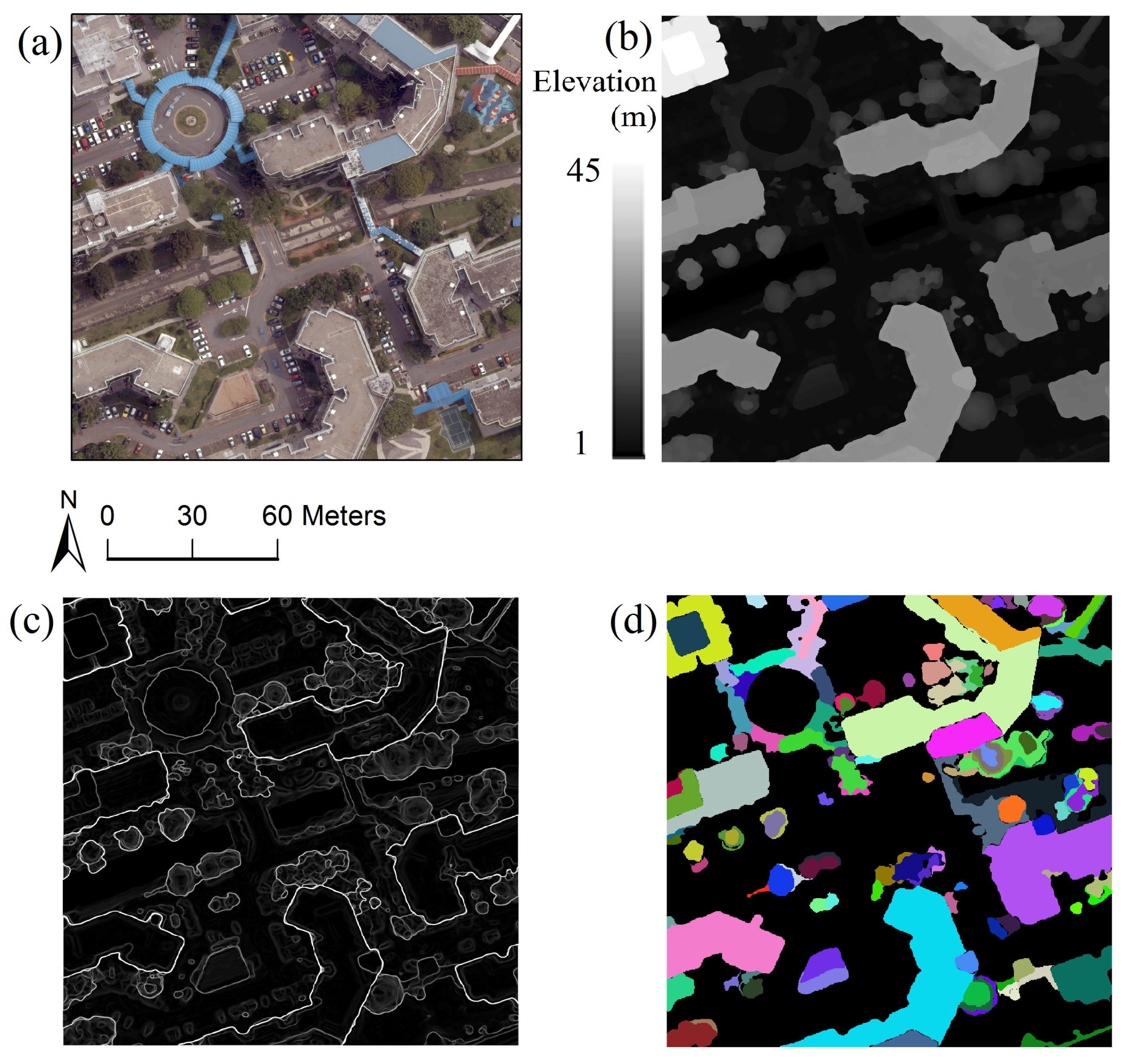
Above-ground object segmentation is a complicated problem which has been studied for years [30,31], but still does not have a general solution. To simplify this problem, we assume all above-ground objects have flat roofs; for example, if a building has two conjoint parts with different heights, then the two parts are treated as two objects. With this assumption we are able to efficiently segment the above-ground objects at the individual level with a simple height clustering algorithm, in which the connected pixels that share similar heights are grouped as one above-ground object. To implement, firstly, we use the DSM to calculate a gradient map which can approximate the above-ground height with respect to surrounding areas. Then, from the highest to the lowest, the connected pixels with height differences within 1 m are sequentially grouped as individual segments. Finally, the segments which have 2.5 m average above-surroundings heights are classified as above-ground objects, as shown in Figure 2.
It is possible that the resulting clusters may contain errors, such as incomplete segments and incorrect above-ground heights, which are mainly in multi-layer objects (e.g., the towers on the roof and the gullies on the ground). To fix these errors, we post-process these segments by simply using neighboring merge technique.
2.2. Side-View Texture Cropping and Selection
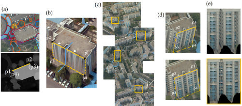
Similar to 3D building façade texture mapping [32], the vertical faces of above-ground objects can be mapped and cropped from oblique images. However, unlike buildings which often have well-defined plane/multi-plane structures in their façades, many above-ground objects, for example, trees, do not possess a specified vertical face. To solve this problem, we convert the boundaries of above-ground segments into polygons with the Douglas–Peucker algorithm [33], thereby creating pseudo vertical faces by cascading the top edges of each object to the ground, as shown in Figure 3, image (a) and (b). In the experiment, only the three longest lines are used to extract side-view textures. As illustrated in Figure 3, image (b), the vertical face is defined as a rectangle with four space points . The upper points are the two ending points of a polygon line with the object height, while the lower points are at the same positions but with ground height. The georeferenced 3D coordinates of the four points in the object space can be acquired from the orthophoto and DSM; thus, their corresponding oblique image coordinates can be calculated via a perspective transformation:
where are the 2D homogeneous coordinates in the oblique image with s as a scale factor, and is a perspective transform matrix which contains the intrinsic and extrinsic camera parameters that are calibrated in the photogrammetric 3D processing. The reader can find more details about the photogrammetry in [34]. As illustrated in Figure 3, image (c) and (d), after this perspective transform, the four points can define a region of the side-view in many multi-view oblique image. To get better side-views for the later feature extractions, we rectify the textures to the front view through a homography transform that maps the points in one image to the corresponding points in the other image (e.g., mapping , , and to the top-left, top-right, bottom-left and bottom right corner of a rectangle image, separately), as shown in Figure 3e. The readers can find more details about homography in [34].
There is in general more than one oblique image that can capture the side-view of an object. To select the best one, we consider three factors: (1) , the quality of the angle between the normal of the face plane and the camera imaging plane, (2) , the quality of the angle between the face normal and the line through camera and face centers, (3) , the proportion of the observable part. Based on these factors, the best side-view is selected by a texture quality measurement:
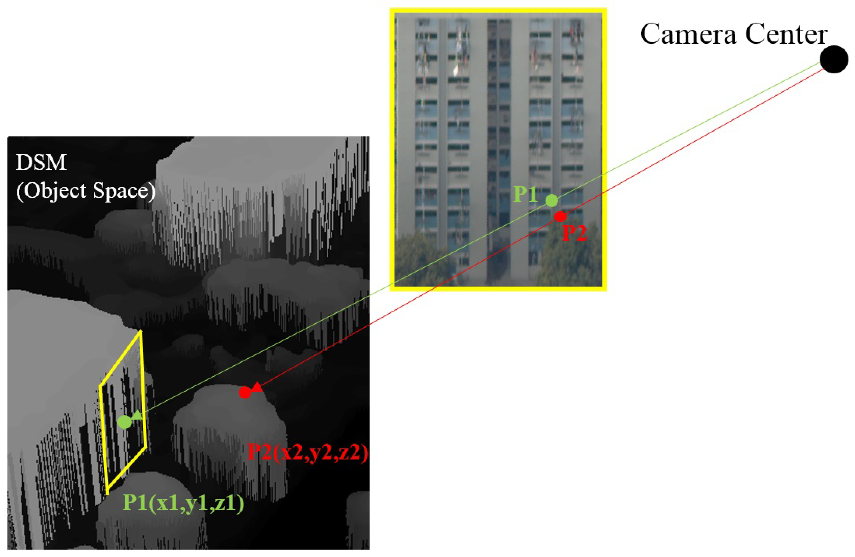
where the measures the quality of side-view f, while the , and are the weights of different quality factors. In the experiment, , and are set as 0.25, 0.25 and 0.5, respectively, as we found the visibility is more important. While the first two factors can be easily calculated, the visibility is complicated to measure due to the fact that occlusions often exist in urban areas. Inspired by a Z-buffer based occlusion detection [29], we examine the visibility with a distance measurement, as illustrated in Figure 4.
For each side-view region in the multi-view oblique images, we can simulate emitting rays from the camera center through the side-view texture and reach the DSM in the object space. If a pixel is not part of the plane (e.g., due to occlusion), as with in Figure 4, we determine that as an invalid pixel for feature extraction. The resulting masked image is shown in Figure 3e.
2.3. Side-View Feature Description
To capture the side-view features, we compute the average color and the standard deviation in R, G, B channels. The histogram of oriented gradients (HOG) [35] and Haar-like features [36,37] are also adopted for the texture description.
HOG descriptor counts occurrences of the gradient orientation in different localized portions of an image with a histogram. By normalizing and concatenating all local HOGs, such as different parts of a human body, we are able to effectively describe object boundaries. In our case, the entire side-view texture is treated as a single patch because there is no dominant or specified distribution. On the other hand, considering that the elements (e.g., windows) in the building façades usually have a regular and repetitive layout, we adopt the rectangle Haar-like features to the side-view images, as has been shown to be highly descriptive. The rectangle Haar-like feature is defined as the difference of the sums of the pixel intensities inside different rectangles. For the side-view textures, a triple-rectangle pattern Haar-like structure (e.g., black-white-black) is designed and used at the vertical and horizontal direction, separately, at 3 different sizes (total 6 feature vectors). Finally, from pixels to blocks, the color, gradient and Haar-like features are combined to describe the side-view for each above-ground segment.
2.4. Classification with Side-View and Top-View
Following the idea of object-based image classification, we first segment the top-view image into small segments as basic classification units. Then, for each segment, top-view features are directly extracted from orthophoto and DSM, while the side-view features are assigned based on the overlaps between the segments and above-ground objects. Finally, with the top-view and side-view features, a random forest classifier is trained to perform the classification.
2.4.1. Image Segmentation with Superpixels
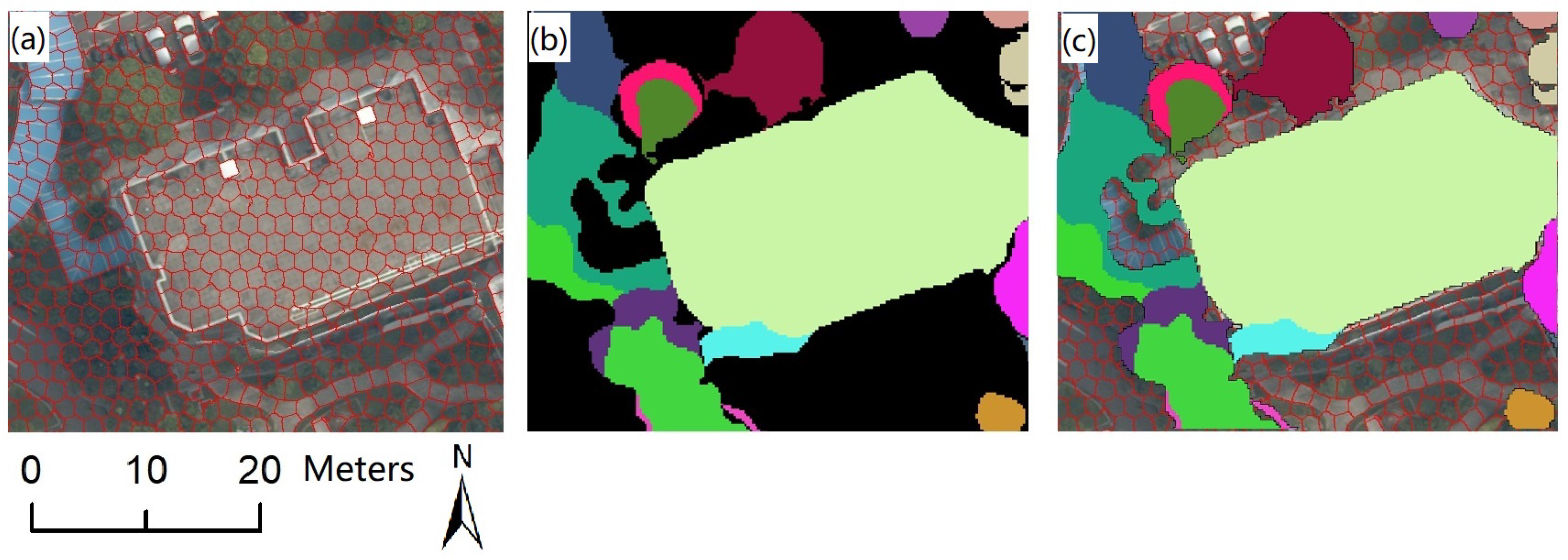
Several image segmentation algorithms have been used for the remote sensing data, such as mean-shift [20,22] and superpixel segmentation [38,39]. Without valuing the shape as a main rule, the mean-shift algorithm can generate well-articulated segments, but the size of segments may vary and the result is sensitive to the algorithm parameters, leading to unpredictable segments. The superpixel algorithm generates compact segments with regular shapes and scales, which are more robust and suitable to associate with the side-view features without unexpected mistakes. Hence, in this study, we generated the SLIC superpixel segments [40] and assigned each segment the side-view features based on its overlap with the above-ground objects, as illustrated in Figure 5. On the other hand, for superpixels which are not in the above-ground areas, their side-view features will be set as zeros.
2.4.2. Classification Workflow
Side-view serves as a piece of complementary information and can be incorporated in any land-cover classification framework with top-view features. Hence, in this work, we directly adopted the framework introduced in [24] which uses a dual morphological top-hat profile (DMTHP) to extract the top-view features and the random forest to classify the segments. More specifically, the top-view features include the DMTHP features extracted from the DSM and brightness and darkness orthophoto images produced by the principal component analysis (PCA) [41]. The DMTHP extracts the spatial features with class-dependent sizes which are adaptively estimated by the training data. This mechanism avoids exhaustive morphology computation of a set of sizes with regular intervals and greatly reduces the dimensions of the feature space. On the other hand, the random forest classifier is widely used for hierarchical feature classifications [42]. The voting strategy of multiple decision trees and the hierarchical examination of the feature elements make this method have high accuracy. The entire classification workflow can be found in Figure 6, and more details about the top-view feature extraction and the random forest classifier can be discovered in [24].
3. Results
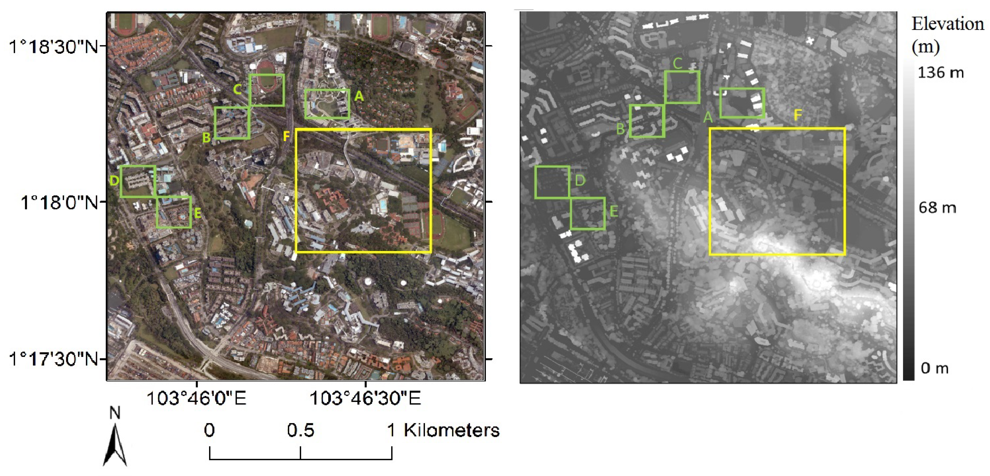
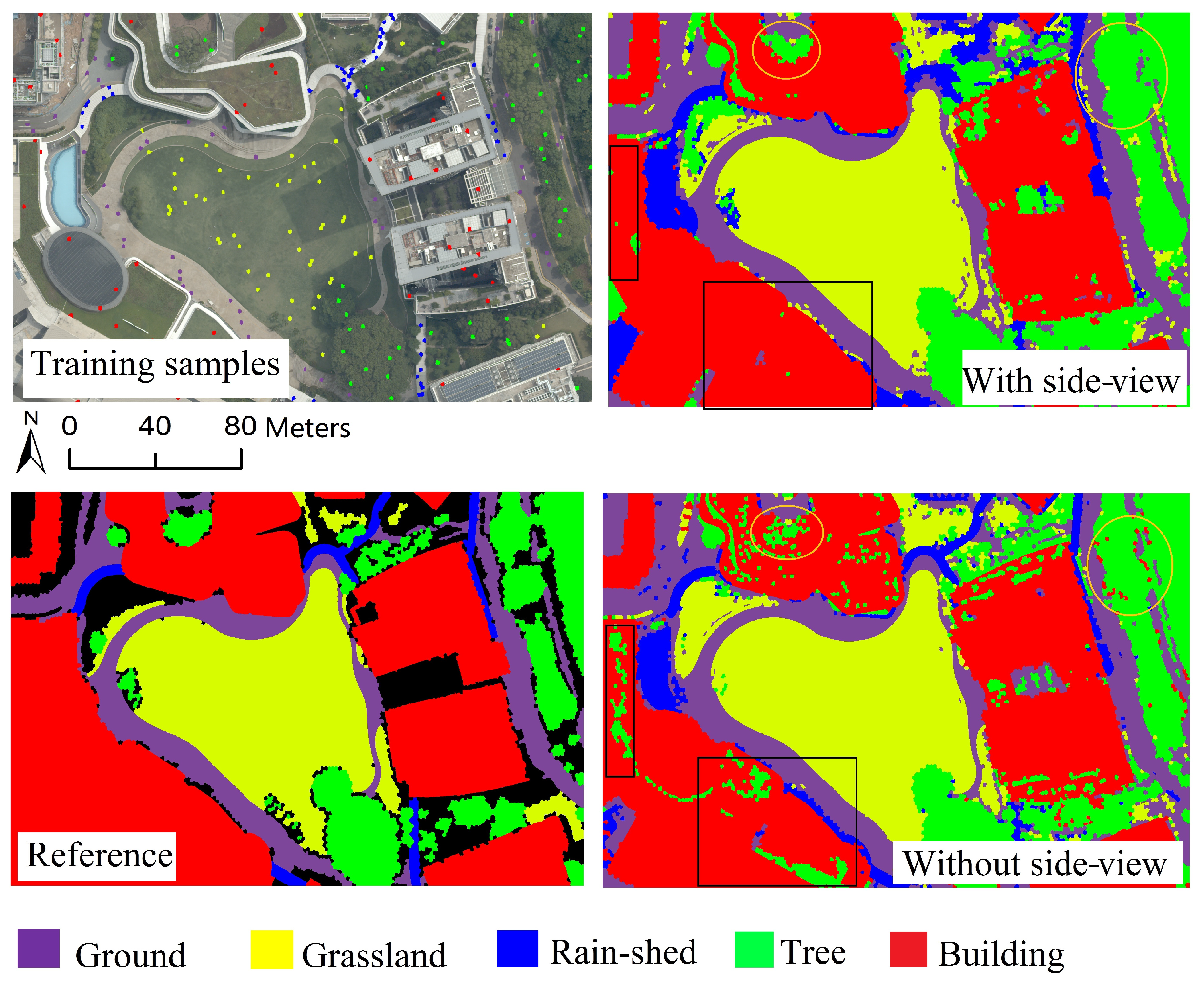
In the experiment, 306 aerial images were used as the study data, including 73 top-view, 64 forward-view, 47 backward-view, 62 left-view and 60 right-view images taken by a 5-head Leica RCD30 airborne camera. The size of all images is 10,336 × 7788 pixels; the four oblique cameras were mounted with a tilt angle of 35 degrees (see Table 1). These images were calibrated by a professional photogrammetric software called Pix4DMapper software (Pix4D SA, Switzerland) which was also used to produce the orthophoto and DSM. The georeferencing accuracy, computed from 9 ground control points, is 2.9 cm. The ground sampling distance (GSD) of the orthophoto and DSM is 7.8 cm. The study area centers around the campus of the National University of Singapore (NUS), where the terrain contains a hilly ridge with tall and low buildings, dense vegetation, roads and manufacturing structures, as illustrated in Figure 7. To analyze the improvement using our method, six sites that each contain all the types with different scenarios were selected. As shown in Figure 7, site A is a complex campus area which includes dormitories, dining halls, study rooms and multi-function buildings. Site B and Site E are residential areas with different types of residential buildings. Site C is a secondary school containing challenging scenarios: the education buildings and a playground are on the roof. Site D is a parking site. Site F, with a complicated land-cover classes, is a much larger area which is used to test the generalization capability of the method.
In this study, the image was classified into (1) ground classes, including road, bare ground and impervious surfaces; (2) grassland; (3) trees; (4) rain-shed including pedestrian overpasses; and (5) building. Other objects, such as cars, rivers/pools and lower vegetation, were not considered. The reference masks of the land-cover were manually drawn by an operator who visually identified the objects in the orthophoto, DSM and oblique images. For each test site (except site F), around 2% of the labeled superpixel segments were used to train the classifier, and more statistics about the experimental setup are listed in Table 2. For the random forest classifier [43], 500 decision trees were used for training, while the number of variables for classification was set as the square root of the feature dimension, which was 35 in the experiment.
3.1. Validation of Above-Ground Object Segmentation
The above-ground object segmentation is an initial and critical step for the side-view information extraction. To validate the above-ground segments, we compared the segments with the reference labels of tree, rain-shed and building. The above-ground segmentation accuracy for the five test sites is shown in Table 3. The evaluation metrics include the accuracy per-class, overall accuracy and commission error, each corresponding to the percentage of correctly identified above-ground pixels in the class, in total, and the miss-classified above-ground pixels, respectively.
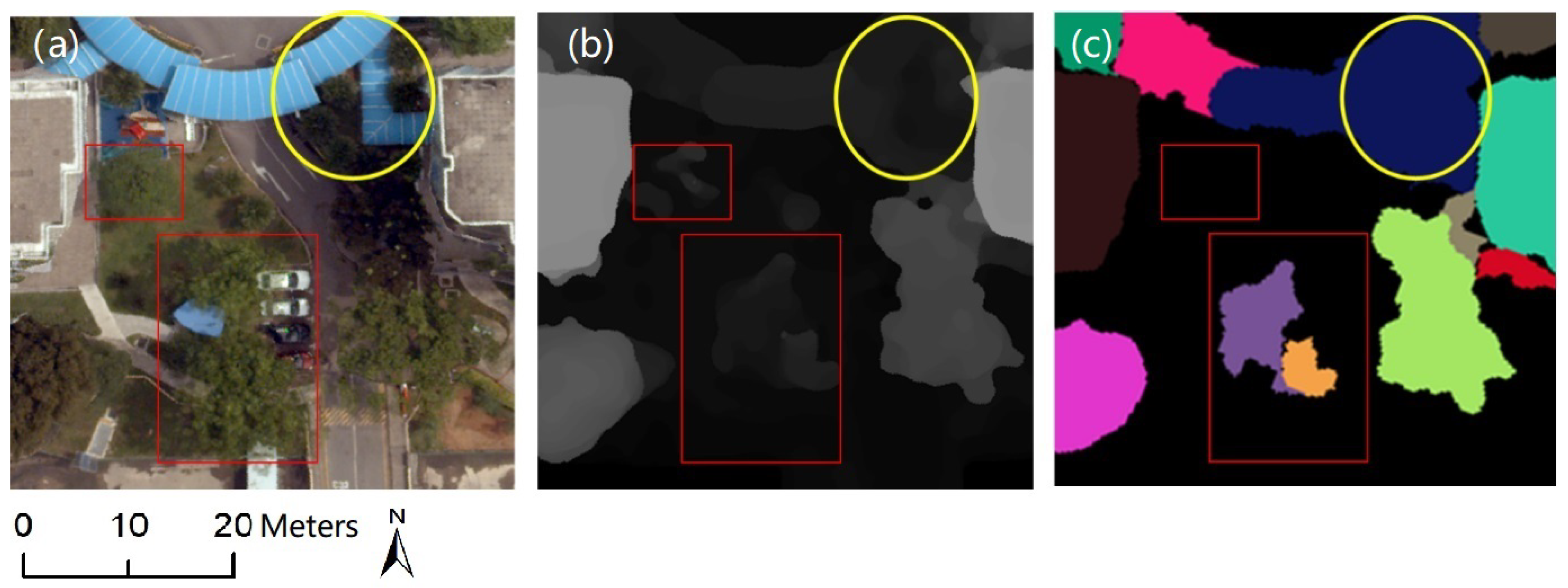
As observed from Table 3, most of the above-ground pixels were successfully segmented (92.7% overall accuracy), and only a few were misclassified (2.42% commission error). For class accuracy, most of the buildings were identified correctly, but with some fuzzy edges. This was mainly caused by the smoothing operation in the generation of DSM, and this operation also reduced the accuracy of the rain-shed, which is low and close to buildings. On the other hand, some pixels of trees were not identified mainly due to the complex structures, such as tree branches, generally not being reconstructed well in current 3D reconstruction approaches, as illustrated by rectangles in Figure 8. In addition, different objects may be segmented as one single object if they are close and have similar heights. This kind of error may make objects have wrong side-views; for instance, the rain-shed would have the side-views of trees, as marked by the circles in Figure 8. However, this error will not significantly impact the final classification, because the side-view is just a piece of complementary information; the top-view features still play an important role in the final classification.
3.2. Classification with Different Samples
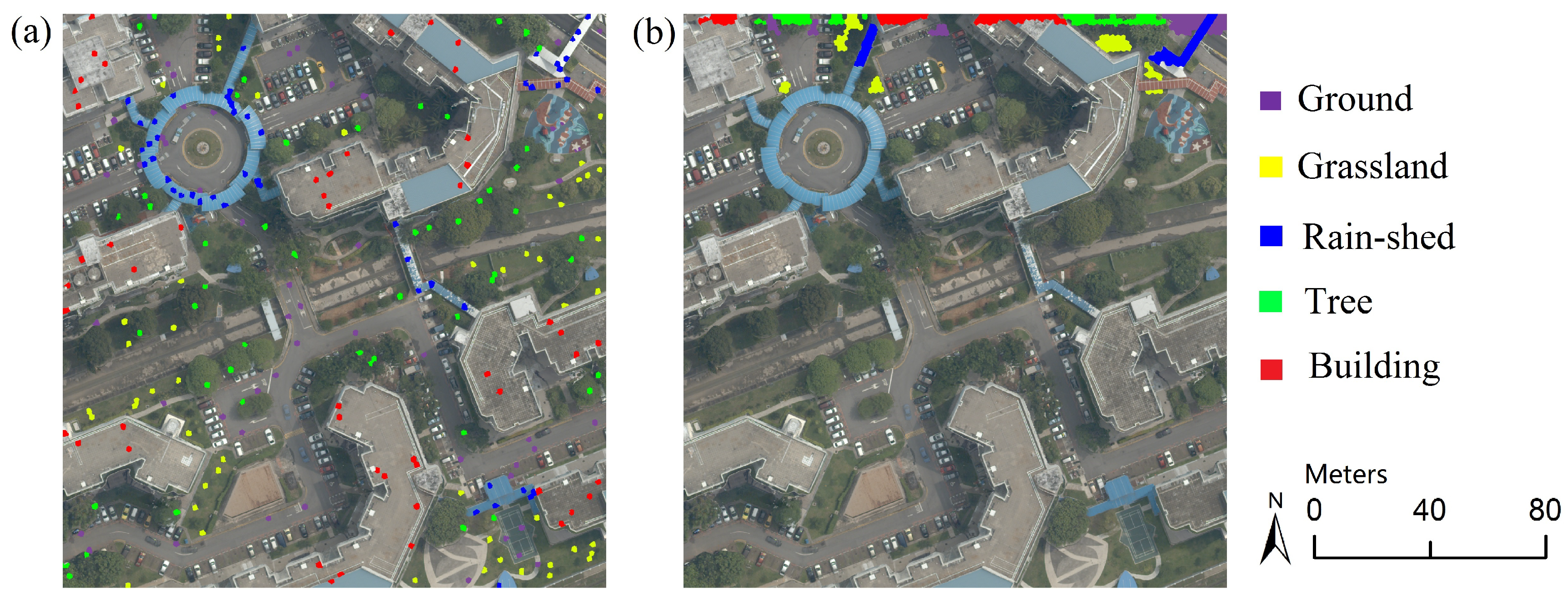
For supervised land-cover classification, the training samples are critical. In practice, depending on the distribution, there are two kinds of samples: (1) evenly collected samples over the entire test site, which we refer to as evenly distributed samples; (2) selectively collected samples covering part of the test site, which we refer to as non-evenly distributed samples. As illustrated in Figure 9a, the evenly distributed samples can offer abundant intra/inter-class information, but they need a considerable amount of labor with scrutiny over the entire image. On the other hand, using non-evenly distributed samples can reduce the manual work and is more efficient at larger scales, but they may not sufficiently represent the data distribution. Considering that these two sample concepts are both very common in practice, we experimented with both of them in our tests.
Classification with Evenly Distributed Samples
The evenly distributed training samples of each class were evenly picked up from reference data with certain intervals. Following the training and prediction process, as described in Section 2.4.2, we performed the classification with/without side-view features, and the results are shown in Table 4 with user accuracy (calculated by taking the total number of correct classifications for a particular class and dividing it by the row total).
As we can observe from Table 4, the results with side-view have higher overall accuracy and Kappa values (on average our method improved 1.1% and 1.5%, separately) which means the side-view information offers useful clues for the land-cover classification. The improvement seems to be limited, as the training samples supply the full capacity of the classifier that is difficult to be further improved. As proven by the experiment, the side-view can still improve the classification if we do not consider the ground objects (ground, grassland) which are not benefited by this extra information. The average per-class accuracy improvement is 1.7%.
As shown from Figure 10, the classification without side-view incorrectly classified some trees into buildings (marked by circles). This misclassification is mainly caused by the fact that many vegetation-covered roofs would make their top-view features have high similarity to the trees. On the other hand, some tropical trees with dense and flat crowns, could have very similar top-view features compared to vegetation-covered roofs. Besides, low vegetation on the roof, as marked by the rectangles in Figure 10, could be misclassified as trees, since it has enough height. However, with the differences in side-views, for example, trees are usually more green and darker, the classifier could identify fewer trees as buildings, and vice versa.
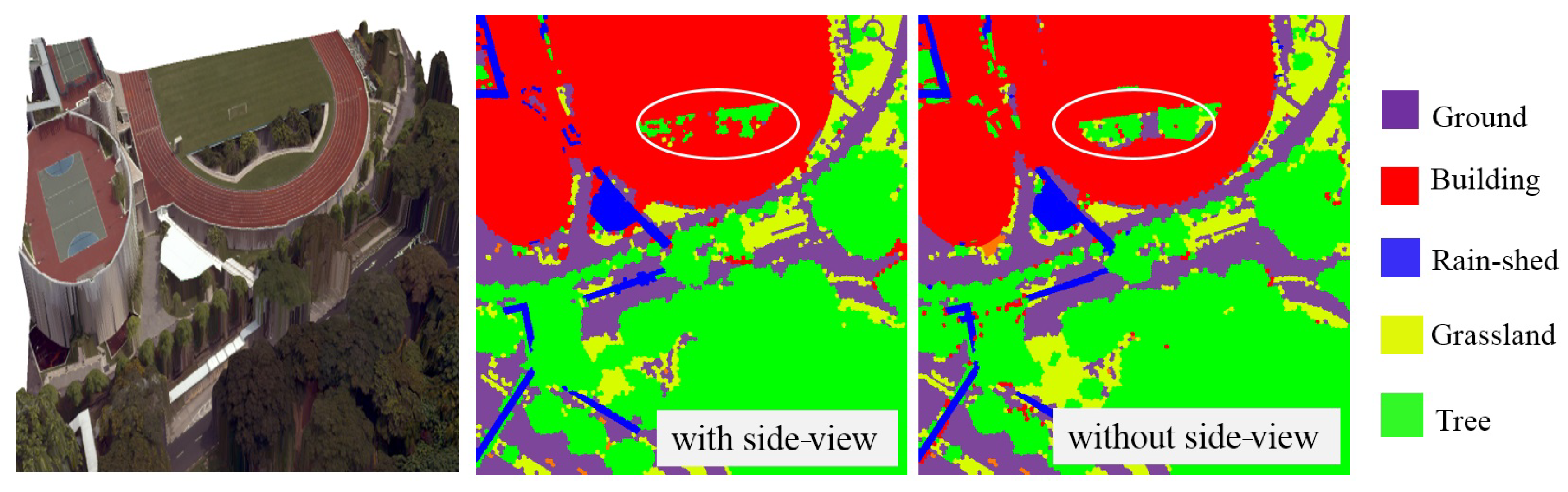
It is possible that the side-view information can be incorrect and damage the classification, as is shown in the circle in Figure 11, where the trees are better identified without side-view information. From the 3D visualization of this area, we observe that the trees are growing through a roof, making the trees have building side-views. This kind of error is mainly caused by the incorrect above-ground segmentation, as we discussed in Section 3.1. Different objects are segmented together, leading to a mismatching of side-views. However, even though the superpixels of trees are assigned with building side-views, their top-views still insure some of them are correctly classified.
3.3. Classification with Non-Evenly Distributed Samples
Usually, the non-evenly distributed samples are more common and practical in real applications. As illustrated in Figure 9b, in the experiment, the non-evenly distributed training samples were generated by selecting training samples of a sub-region of an image. With the same training and prediction process, the user accuracies of classification with/without side-view features are given in Table 5.
As compared to the results of evenly distributed training samples, the non-evenly distributed samples have a degraded performance (around 10% and 16% lower overall accuracy for classification with/without side-view, separately). It is well-understood such a training sample selection process may not sufficiently represent the data distribution. However, in such a situation, the side-view still improved the average overall accuracy by 5.6%, the building was even improved by 9.3%. However, in sites B, D and E, the side-view information reduced the accuracy of the tree class. Trees close to buildings and the rain-shed could have unstable side-view features due to the occlusion and the 3D structure of some trees not being reconstructed, which may introduce errors in tree recognition. Thus, if with only limited training samples, this instability may damage the training leading to unreliable predictions. Nevertheless, with high quality training samples, or even limited-quality ones, the involvement of side-views can still greatly improve the land-cover classification, as demonstrated by the classification of the buildings.
Generalization Ability of Side-View Information
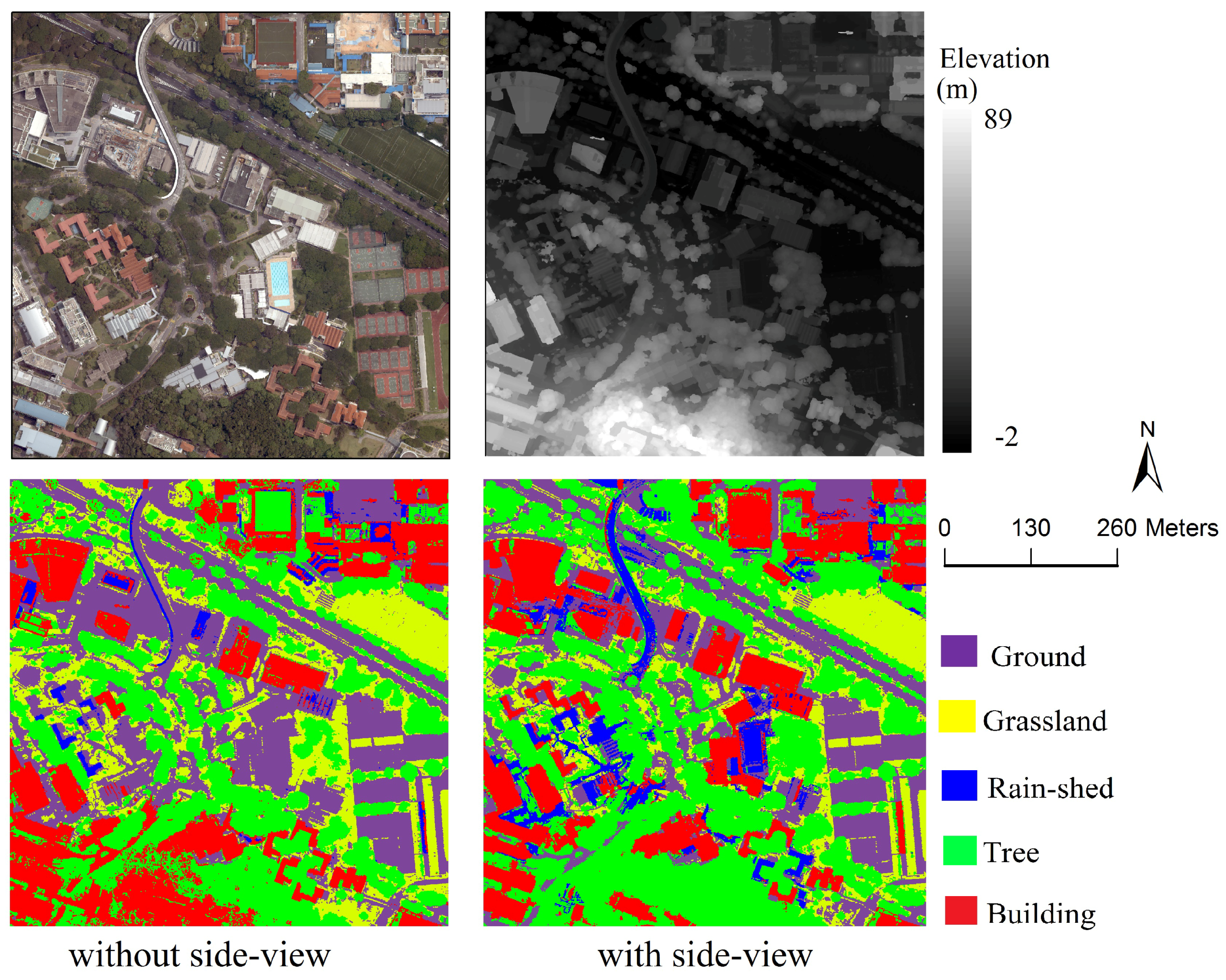
To further analyze the generalization ability of the side-view information, we experimented with the trained classifier at a much larger area (site F which is 16 times larger than other sites) at the center of NUS campus. Due to the very high resolution of this data (GSD is 7.8 cm, contains pixels), we down sampled it to one-third of the original size. In this area, a total of 180,152 superpixel segments were generated, containing short and high buildings, tropical trees with smooth canopies, interchanging roads and constructions along the ridge of a hill. In the experiment, the classifier was trained by the reference data of previously mentioned five test sites, and the classification results (with/without side-view) are shown in Figure 12 and Table 6.
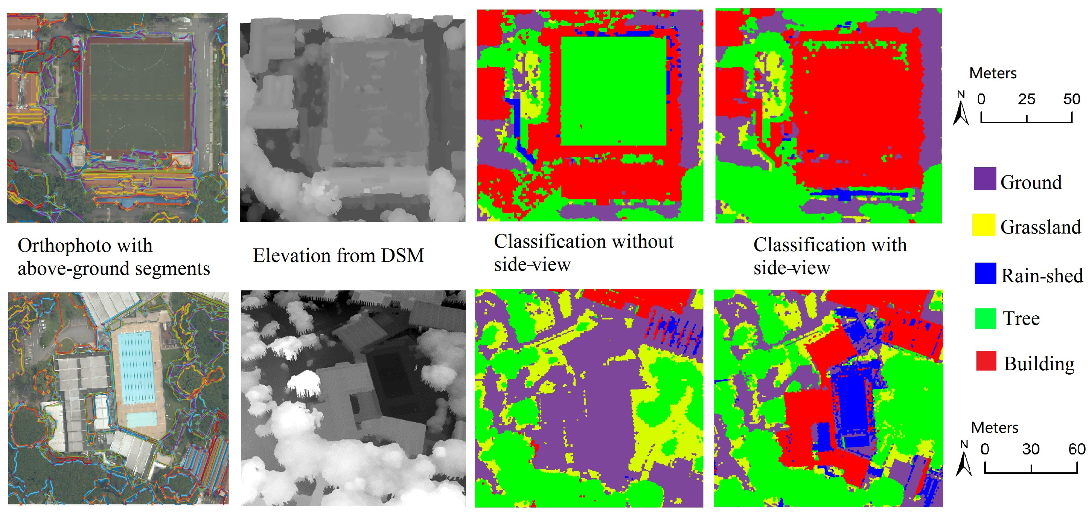
In Figure 12, we can observe that the side-view has greatly improved the classification accuracy: (1) With the side-view, the overall accuracy and Kappa have been improved by 14.5% and 18.9%. (2) For the above-ground objects, the overall accuracy of the building and rain-shed have been improved by 28.37% and 34.53%, leading to a large category average improvement of 26.2% (including the tree). If the classification is performed without side-view information, many buildings are identified as ground, while some trees are identified as buildings. This site (F) contains a complicated area with various man-made objects and dense trees crossing a hill with large topographic relief (more than 90 meters). In Singapore, many buildings with green/playground roofs can be challenging and often mislead the algorithm to produce incorrect results, for example, by classifying green roofs to the tree class. Especially, if the buildings are surrounded by trees or at the hillside, they could be classified as ground due to the relief of the DSM, as shown in Figure 13. Unlike the top-view or the elevation features that can be sensitive to the DSM relief changes, the side-view features are much more consistent and robust to varying scenarios. For the two examples illustrated in Figure 13, with the side-view information, the buildings at the hillside can be correctly classified, as can the one with a playground roof.
As mentioned above, the classification could be sensitive to the training samples. To analyze that, we changed the training samples by alternatively removing samples site by site. In other words, we alternatively selected samples from the four of five test sites (A–E) and tested the performance robustness with varying training samples. The results with accuracy and Kappa values, and their average (Avg.) and standard deviation (Sd.) values can be found in Table 7.
From Table 7, we observe the classification with side-view is more robust to the change of training data, and has smaller standard deviations for both overall accuracy and Kappa. We can find the training samples from site A and D are crucial for the top-view features, as the classifications have obviously decreased without their training data, indicating the top-view features are sensitive to training samples. On the contrary, with the side-view information, the performance is stable, indicating the side-view features are more steady and robust to the randomness of training samples.
4. Discussion
As demonstrated in the experiments, the side-view information can steadily improve the classification performance. However, there are still some issues we need to further discuss. Firstly, as mentioned, the above-ground objects segmentation which decides the boundaries of each object and the corresponding textures is critical for the side-view information extraction. In this study, we tried several methods to segment the above-ground objects [30,31]. However, it is a quite complicated problem and we did not find an obviously better solution than the adopted height-grouping algorithm. There are two issues in the segmentation, incorrect boundaries and under-segmentation of multi-objects. We observed the first issue will not damage the side-view information due to the fact that incorrect boundary can still offer appropriate locations for the side-view texture. On the other hand, the under-segmentation of multi-objects cannot be ignored. It will confuse the side-views between different objects and classes. To solve this, the color difference could be considered, with the height-grouping in the above-ground object segmentation. However, this introduction usually causes over-segmentation, fragmenting objects into pieces and hindering the side-view extraction. The deep learning neural networks [44,45,46] could be promising solutions which we would explore in the future.
The selection of training samples is another important fact that decides the classification performance. As mentioned in the results, the evenly-distributed samples have much better performance than non-evenly distributed ones, because this kind of training sample can supply category-level features, instead of object-level ones. The classifier can be well trained with complete data, leading to ideal performance which is hard to be further improved. On the contrary, the dataset underrepresented by the non-evenly distributed samples and the classifier training will be partial, leading to poor classification. This is mainly caused by the high intra-class variability of top-view features that makes the classifier vulnerable to untrained data. As shown in the results, the side-view information is more robust and consistent. This also inspires us to consider multiple dimension features for object classification and recognition in future works.
In our experiment, we also observed a few misclassified areas, for example, many rain-sheds were not classified correctly. There are two main challenges for rain-shed identification: the rain-sheds are short in height and are close to the buildings and trees, the side-view of which might be misleading. On the other hand, we found the ground objects have slightly worse classification results with the side-view. This is mainly caused by the errors in the above-ground segmentation. Many ground areas are wrongly segmented as above-ground objects due to the limited accuracy of the DSM. Particularly, objects in slope may be mixed with ground area in the slope. Hence, how to extract and use side-view information still needs further development.
5. Conclusions
In this study, we aimed to fully utilize the possible information acquired by the oblique aerial image and analyze the potential of using side-view information for land-cover classification. To contribute the side-view information to the top-view segments, we proposed a side-view information extraction method, described in Section 2. More specially, to get the side-view information, we first segment out the above-ground segments with a height grouping algorithm. Then, based on the boundaries which have been converted to polygons, their 3D vertical side-view planes are defined. With the perspective transformation, the side-view textures of above-ground objects can be cropped and selected from oblique images. Finally, from these oblique textures, the side-view information, including color, HoG and Haar-like features, are extracted as extra information for the classification. Our experiment in different test sites shows that the side-view can steady improve the classification accuracy either with evenly distributed or non-evenly distributed training samples (by 1.1% and 5.6%, respectively). Also, the generalization ability of the side-view is evaluated and demonstrated as a 14.5% accuracy improvement as tested at a larger and untrained area.
Even though the side-view features show strong consistency and high robust to different sites, the training samples are still critical to the classification. In our experiments we observed some commission errors, which were primarily from incorrect segmentation results, which should be further improved.
Author Contributions
R.Q. and C.X. initiated this research. C.X. performed the experiment, and X.L. contributed to part of the data processing. C.X. wrote this manuscript; R.Q. and X.L. helped with the edit. All authors have read and agreed to the published version of the manuscript.
Funding
This material is based on research/work supported by the National Research Foundation under Virtual Singapore, award number NRF2015VSG-AA3DCM001-024.
Acknowledgments
We are grateful to Singapore Land Authority (SLA) for their great support on multi-sensor data.
Conflicts of Interest
The authors declare no conflict of interest.
References
- Audebert, N.; Le Saux, B.; Lefèvre, S. Beyond RGB: Very high resolution urban remote sensing with multimodal deep networks. ISPRS J. Photogramm. Remote Sens. 2018, 140, 20–32. [Google Scholar] [CrossRef] [Green Version]
- Inglada, J. Automatic recognition of man-made objects in high resolution optical remote sensing images by SVM classification of geometric image features. ISPRS J. Photogramm. Remote Sens. 2007, 62, 236–248. [Google Scholar] [CrossRef]
- Matikainen, L.; Karila, K.; Hyyppä, J.; Litkey, P.; Puttonen, E.; Ahokas, E. Object-based analysis of multispectral airborne laser scanner data for land cover classification and map updating. ISPRS J. Photogramm. Remote Sens. 2017, 128, 298–313. [Google Scholar] [CrossRef]
- Ma, L.; Li, M.; Ma, X.; Cheng, L.; Du, P.; Liu, Y. A review of supervised object-based land-cover image classification. ISPRS J. Photogramm. Remote Sens. 2017, 130, 277–293. [Google Scholar] [CrossRef]
- Zhang, C.; Pan, X.; Li, H.; Gardiner, A.; Sargent, I.; Hare, J.; Atkinson, P.M. A hybrid MLP-CNN classifier for very fine resolution remotely sensed image classification. ISPRS J. Photogramm. Remote Sens. 2018, 140, 133–144. [Google Scholar] [CrossRef] [Green Version]
- Zhang, C.; Sargent, I.; Pan, X.; Li, H.; Gardiner, A.; Hare, J.; Atkinson, P.M. Joint Deep Learning for land cover and land use classification. Remote Sens. Environ. 2019, 221, 173–187. [Google Scholar] [CrossRef] [Green Version]
- Rouse, J., Jr.; Haas, R.; Schell, J.; Deering, D. Monitoring Vegetation Systems in the Great Plains with ERTS; NASA Special Publication: Washington, DC, USA, 1974.
- McFeeters, S.K. The use of the Normalized Difference Water Index (NDWI) in the delineation of open water features. Int. J. Remote Sens. 1996, 17, 1425–1432. [Google Scholar] [CrossRef]
- Salomonson, V.V.; Appel, I. Estimating fractional snow cover from MODIS using the normalized difference snow index. Remote Sens. Environ. 2004, 89, 351–360. [Google Scholar] [CrossRef]
- Lampkin, D.J.; Yool, S.R. Monitoring mountain snowpack evolution using near-surface optical and thermal properties. Hydrol. Process. 2004, 18, 3527–3542. [Google Scholar] [CrossRef]
- Rogers, A.; Kearney, M. Reducing signature variability in unmixing coastal marsh Thematic Mapper scenes using spectral indices. Int. J. Remote Sens. 2004, 25, 2317–2335. [Google Scholar] [CrossRef]
- Huang, P.S.; Tu, T.M. A target fusion-based approach for classifying high spatial resolution imagery. In Proceedings of the IEEE Workshop on Advances in Techniques for Analysis of Remotely Sensed Data, Greenbelt, UK, 27–28 October 2003; pp. 175–181. [Google Scholar]
- Zhang, L.; Huang, X.; Huang, B.; Li, P. A pixel shape index coupled with spectral information for classification of high spatial resolution remotely sensed imagery. IEEE Trans. Geosci. Remote Sens. 2006, 44, 2950–2961. [Google Scholar] [CrossRef]
- Benediktsson, J.A.; Palmason, J.A.; Sveinsson, J.R. Classification of hyperspectral data from urban areas based on extended morphological profiles. IEEE Trans. Geosci. Remote Sens. 2005, 43, 480–491. [Google Scholar] [CrossRef]
- Huang, X.; Lu, Q.; Zhang, L. A multi-index learning approach for classification of high-resolution remotely sensed images over urban areas. ISPRS J. Photogramm. Remote Sens. 2014, 90, 36–48. [Google Scholar] [CrossRef]
- Ouma, Y.O.; Tetuko, J.; Tateishi, R. Analysis of co-occurrence and discrete wavelet transform textures for differentiation of forest and non-forest vegetation in very-high-resolution optical-sensor imagery. Int. J. Remote Sens. 2008, 29, 3417–3456. [Google Scholar] [CrossRef]
- Huang, X.; Zhang, L.; Li, P. Classification and extraction of spatial features in urban areas using high-resolution multispectral imagery. IEEE Geosci. Remote Sens. Lett. 2007, 4, 260–264. [Google Scholar] [CrossRef]
- Fauvel, M.; Chanussot, J.; Benediktsson, J.A. A spatial–spectral kernel-based approach for the classification of remote-sensing images. Pattern Recognit. 2012, 45, 381–392. [Google Scholar] [CrossRef]
- Pingel, T.J.; Clarke, K.C.; McBride, W.A. An improved simple morphological filter for the terrain classification of airborne LIDAR data. ISPRS J. Photogramm. Remote Sens. 2013, 77, 21–30. [Google Scholar] [CrossRef]
- Huang, X.; Zhang, L. An adaptive mean-shift analysis approach for object extraction and classification from urban hyperspectral imagery. IEEE Trans. Geosci. Remote Sens. 2008, 46, 4173–4185. [Google Scholar] [CrossRef]
- Huang, X.; Zhang, L.; Gong, W. Information fusion of aerial images and LIDAR data in urban areas: Vector-stacking, re-classification and post-processing approaches. Int. J. Remote Sens. 2011, 32, 69–84. [Google Scholar] [CrossRef]
- Qin, R.; Huang, X.; Gruen, A.; Schmitt, G. Object-based 3-D building change detection on multitemporal stereo images. IEEE J. Sel. Top. Appl. Earth Obs. Remote Sens. 2015, 8, 2125–2137. [Google Scholar] [CrossRef]
- Xiao, C.; Qin, R.; Xie, X.; Huang, X. Individual Tree Detection and Crown Delineation with 3D Information from Multi-view Satellite Images. Photogramm. Eng. Remote Sens. 2019, 85, 55–63. [Google Scholar] [CrossRef] [Green Version]
- Zhang, Q.; Qin, R.; Huang, X.; Fang, Y.; Liu, L. Classification of ultra-high resolution orthophotos combined with DSM using a dual morphological top hat profile. Remote Sens. 2015, 7, 16422–16440. [Google Scholar] [CrossRef] [Green Version]
- Teo, T.A.; Wu, H.M. Analysis of land cover classification using multi-wavelength LiDAR system. Appl. Sci. 2017, 7, 663. [Google Scholar] [CrossRef] [Green Version]
- Fradkin, M.; Maıtre, H.; Roux, M. Building detection from multiple aerial images in dense urban areas. Comput. Vis. Image Underst. 2001, 82, 181–207. [Google Scholar] [CrossRef]
- Morgan, M.; Habib, A. Interpolation of lidar data and automatic building extraction. In ACSM-ASPRS Annual Conference Proceedings; Citeseer: Princeton, NJ, USA, 2002; pp. 432–441. [Google Scholar]
- Lin, Y.; Jiang, M.; Yao, Y.; Zhang, L.; Lin, J. Use of UAV oblique imaging for the detection of individual trees in residential environments. Urban For. Urban Green. 2015, 14, 404–412. [Google Scholar] [CrossRef]
- Rau, J.Y.; Jhan, J.P.; Hsu, Y.C. Analysis of oblique aerial images for land cover and point cloud classification in an urban environment. IEEE Trans. Geosci. Remote Sens. 2014, 53, 1304–1319. [Google Scholar] [CrossRef]
- Luethje, F.; Tiede, D.; Eisank, C. Terrain extraction in built-up areas from satellite stereo-imagery-derived surface models: A stratified object-based approach. ISPRS Int. J. Geo-Inf. 2017, 6, 9. [Google Scholar] [CrossRef] [Green Version]
- Piltz, B.; Bayer, S.; Poznanska, A.M. Volume based DTM generation from very high resolution photogrammetric DSMs. Int. Arch. Photogramm. Remote Sens. Spat. Inf. Sci. 2016, 41, 83–90. [Google Scholar] [CrossRef]
- Frueh, C.; Sammon, R.; Zakhor, A. Automated texture mapping of 3D city models with oblique aerial imagery. In Proceedings of the 2nd International Symposium on 3D Data Processing, Visualization and Transmission, Thessaloniki, Greece, 9 September 2004; pp. 396–403. [Google Scholar]
- Douglas, D.H.; Peucker, T.K. Algorithms for the reduction of the number of points required to represent a digitized line or its caricature. Cartogr. Int. J. Geogr. Inf. Geovis. 1973, 10, 112–122. [Google Scholar] [CrossRef] [Green Version]
- Hartley, R.; Zisserman, A. Multiple View Geometry in Computer Vision; Cambridge University Press: Cambridge, UK, 2003. [Google Scholar]
- Dalal, N.; Triggs, B. Histograms of oriented gradients for human detection. In Proceedings of the 2005 IEEE Computer Society Conference on Computer Vision and Pattern Recognition (CVPR’05), San Diego, CA, USA, 20–25 June 2005. [Google Scholar]
- Crow, F.C. Summed-area tables for texture mapping. In Proceedings of the 11th Annual Conference on Computer Graphics and iNteractive Techniques, Minneapolis, MN, USA, 23–27 July 1984; Volume 18, pp. 207–212. [Google Scholar]
- Viola, P.; Jones, M. Rapid object detection using a boosted cascade of simple features. CVPR (1) 2001, 1, 3. [Google Scholar]
- Audebert, N.; Le Saux, B.; Lefevre, S. How useful is region-based classification of remote sensing images in a deep learning framework? In Proceedings of the 2016 IEEE International Geoscience and Remote Sensing Symposium (IGARSS), Beijing, China, 10–15 July 2016; pp. 5091–5094. [Google Scholar]
- Wu, Z.; Hu, Z.; Fan, Q. Superpixel-based unsupervised change detection using multi-dimensional change vector analysis and SVM-based classification. ISPRS Ann. Photogramm. Remote Sens. Spat. Inf. Sci. 2012, 7, 257–262. [Google Scholar] [CrossRef] [Green Version]
- Achanta, R.; Shaji, A.; Smith, K.; Lucchi, A.; Fua, P.; Süsstrunk, S. SLIC superpixels compared to state-of-the-art superpixel methods. IEEE Trans. Pattern Anal. Mach. Intell. 2012, 34, 2274–2282. [Google Scholar] [CrossRef] [PubMed] [Green Version]
- Wold, S.; Esbensen, K.; Geladi, P. Principal component analysis. Chemom. Intell. Lab. Syst. 1987, 2, 37–52. [Google Scholar] [CrossRef]
- Sun, X.; Lin, X.; Shen, S.; Hu, Z. High-resolution remote sensing data classification over urban areas using random forest ensemble and fully connected conditional random field. ISPRS Int. J. Geo-Inf. 2017, 6, 245. [Google Scholar] [CrossRef] [Green Version]
- Pal, M. Random forest classifier for remote sensing classification. Int. J. Remote Sens. 2005, 26, 217–222. [Google Scholar] [CrossRef]
- Kampffmeyer, M.; Salberg, A.B.; Jenssen, R. Semantic segmentation of small objects and modeling of uncertainty in urban remote sensing images using deep convolutional neural networks. In Proceedings of the IEEE Conference on Computer Vision and Pattern Recognition Workshops, Las Vegas, NV, USA, 26 June–1 July 2016; pp. 1–9. [Google Scholar]
- Marmanis, D.; Wegner, J.D.; Galliani, S.; Schindler, K.; Datcu, M.; Stilla, U. Semantic segmentation of aerial images with an ensemble of CNNs. ISPRS Ann. Photogramm. Remote Sens. Spat. Inf. Sci. 2016, 3, 473. [Google Scholar] [CrossRef] [Green Version]
- Wang, H.; Wang, Y.; Zhang, Q.; Xiang, S.; Pan, C. Gated convolutional neural network for semantic segmentation in high-resolution images. Remote Sens. 2017, 9, 446. [Google Scholar] [CrossRef] [Green Version]
Figure 1.
The top-view and side-view of two above-ground objects. When the objects have confusing top-views (left), they may be more recognizable from the side-view (right).
Figure 1.
The top-view and side-view of two above-ground objects. When the objects have confusing top-views (left), they may be more recognizable from the side-view (right).

Figure 2.
Segmentation of above-ground objects with height clustering. (a,b) Orthophotos and the digital surface model (DSM) of a study area; (c,d) the gradient map and the final segments (colors are used to show different segments).
Figure 2.
Segmentation of above-ground objects with height clustering. (a,b) Orthophotos and the digital surface model (DSM) of a study area; (c,d) the gradient map and the final segments (colors are used to show different segments).

Figure 3.
The side-view texture extraction from multi-view oblique images. (a) An example of above-ground object polygon boundaries and its DSM, while the next image (b) shows one of its 3D vertical faces. Next are possible projections of multi-view oblique images (c). Finally, (d,e) the original and rectified side-view textures are shown, while the yellow rectangle in image (e) marks the best texture.

Figure 4.
An illustration of the occlusion detection through Z-buffer with the DSM. A texture point (e.g., ), must be close to the side-view plane (yellow rectangle) in the object space; otherwise (e.g., which is pointing at a tree) it should be an occlusion point.
Figure 4.
An illustration of the occlusion detection through Z-buffer with the DSM. A texture point (e.g., ), must be close to the side-view plane (yellow rectangle) in the object space; otherwise (e.g., which is pointing at a tree) it should be an occlusion point.

Figure 5.
The assignment of side-view features for each superpixel segment. (a) The orthophoto with superpixels. (b) Above-ground segments (color blocks) and (c) their overlap.
Figure 5.
The assignment of side-view features for each superpixel segment. (a) The orthophoto with superpixels. (b) Above-ground segments (color blocks) and (c) their overlap.

Figure 6.
The proposed workflow for the land-cover classification.

Figure 7.
The study area around National University of Singapore (NUS) campus with six experiment sites marked by rectangles.
Figure 7.
The study area around National University of Singapore (NUS) campus with six experiment sites marked by rectangles.

Figure 8.
The illustration of the errors in above-ground object segmentation. The orthophoto (a), DSM (b), and above-ground segments with different colors (c). Rectangles mark the missed trees while the circles mark a segment which contains multiple objects.
Figure 8.
The illustration of the errors in above-ground object segmentation. The orthophoto (a), DSM (b), and above-ground segments with different colors (c). Rectangles mark the missed trees while the circles mark a segment which contains multiple objects.

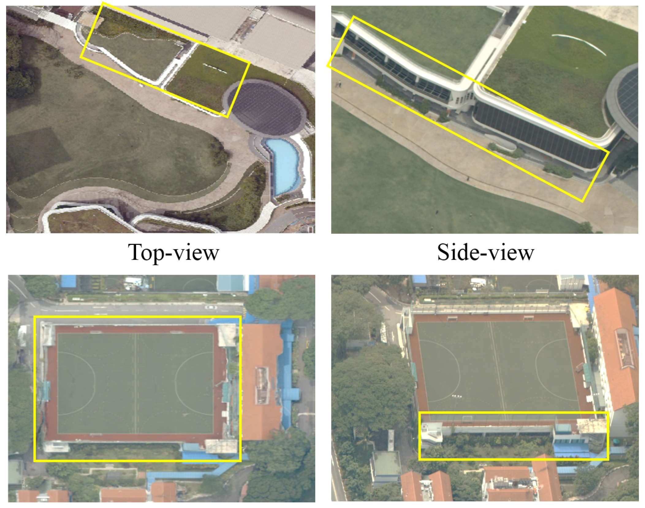
Figure 9.
Training samples with different collection methods. (a) Evenly distributed samples; (b) Non-evenly distributed samples.
Figure 9.
Training samples with different collection methods. (a) Evenly distributed samples; (b) Non-evenly distributed samples.

Figure 10.
Classification results in site A.

Figure 11.
Classification results in site C.

Figure 12.
Land-cover classification at the center of NUS campus.

Figure 13.
The classifications of two complicated areas. The lower row shows examples of hillside buildings, while upper row shows a building with a playground roof.
Figure 13.
The classifications of two complicated areas. The lower row shows examples of hillside buildings, while upper row shows a building with a playground roof.


Table 1.
The statistics of the images data.
| Leica RCD30 Airborne Camera (Altitude: 800 to 900 m) | Top-View | Side-View (Oblique Images) |
|---|---|---|
| Image size | 10,336 pixels × 7788 pixels | 10,336 pixels × 7788 pixels |
| Angle | 0 | 35 degree |
| Average ground sample distance | 0.078 m | 0.078 m |
Table 2.
The statistics of training and test samples.
| Site | A | B | C | D | E | |
|---|---|---|---|---|---|---|
| Training samples for each class | Ground | 50 | 51 | 50 | 51 | 50 |
| Grassland | 50 | 51 | 49 | 51 | 44 | |
| Rain-shed | 49 | 52 | 49 | 27 | 51 | |
| Tree | 50 | 51 | 50 | 50 | 51 | |
| building | 51 | 50 | 51 | 50 | 50 | |
| Total training samples | 250 | 249 | 249 | 229 | 246 | |
| Total test samples | 14,791 | 7883 | 7883 | 8099 | 6006 | |
| Total segments | 17,285 | 11,237 | 11,237 | 11,232 | 11,236 | |
| Percentage | 1.45 % | 2.27 % | 2.22 % | 2.04 % | 2.19 % |
Table 3.
The accuracy of the above-ground segmentation.
| Site | Class Accuracy (%) | Overall Accuracy (%) | Commission Error (%) | ||
|---|---|---|---|---|---|
| Rain-shed | Tree | Building | |||
| A | 97.82 | 83.25 | 96.16 | 93.44 | 1.32 |
| B | 94.64 | 85.02 | 99.14 | 94.55 | 2.92 |
| C | 89.05 | 94.66 | 99.64 | 96.79 | 0.39 |
| D | 99.92 | 63.17 | 98.81 | 85.33 | 4.91 |
| E | 79.42 | 84.80 | 98.40 | 93.71 | 2.54 |
| Avg. | 92.17 | 82.18 | 98.43 | 92.76 | 2.42 |
Table 4.
The land-cover classification user accuracy (%) with evenly distributed samples.
| Site | Side-View | Ground | Grassland | Rain-Shed | Tree | Building | Overall Accuracy | Kappa |
|---|---|---|---|---|---|---|---|---|
| A | Yes | 93.52 | 95.70 | 93.67 | 94.11 | 90.63 | 92.65 | 89.46 |
| No | 92.40 | 95.93 | 92.64 | 87.30 | 89.12 | 90.83 | 86.85 | |
| B | Yes | 88.01 | 85.54 | 93.15 | 93.12 | 96.42 | 92.06 | 89.52 |
| No | 85.34 | 86.95 | 91.58 | 92.09 | 96.42 | 91.22 | 88.44 | |
| C | Yes | 92.74 | 94.61 | 96.33 | 96.96 | 99.45 | 97.26 | 95.86 |
| No | 92.66 | 94.62 | 95.70 | 97.48 | 99.12 | 97.30 | 95.93 | |
| D | Yes | 93.04 | 95.07 | 90.24 | 89.95 | 97.27 | 92.73 | 90.64 |
| No | 92.14 | 94.43 | 88.65 | 86.20 | 90.87 | 90.45 | 87.67 | |
| E | Yes | 95.08 | 95.78 | 88.17 | 92.71 | 96.30 | 95.15 | 92.37 |
| No | 94.83 | 95.14 | 88.17 | 91.87 | 95.87 | 94.71 | 91.68 | |
| Avg. | Yes | 92.48 | 93.34 | 92.31 | 93.37 | 96.01 | 93.97 | 91.57 |
| No | 91.47 | 93.41 | 91.35 | 90.99 | 94.28 | 92.90 | 90.11 |
Table 5.
The user accuracies (%) of land-cover classification with non-evenly distributed training samples.
Table 5.
The user accuracies (%) of land-cover classification with non-evenly distributed training samples.
| Site | Side-View | Ground | Grassland | Rain-Shed | Tree | Building | Overall Accuracy | Kappa |
|---|---|---|---|---|---|---|---|---|
| A | Yes | 41.59 | 97.85 | 68.12 | 77.66 | 91.09 | 83.03 | 75.16 |
| No | 42.73 | 97.95 | 59.51 | 74.91 | 64.46 | 69.67 | 58.17 | |
| B | Yes | 83.27 | 94.32 | 79.80 | 86.15 | 96.34 | 89.73 | 86.12 |
| No | 84.94 | 92.92 | 81.07 | 88.76 | 88.37 | 87.49 | 83.16 | |
| C | Yes | 95.79 | 87.47 | 84.11 | 99.31 | 91.92 | 95.03 | 92.46 |
| No | 91.66 | 87.93 | 94.99 | 94.52 | 85.20 | 90.23 | 85.19 | |
| D | Yes | 63.85 | 97.17 | 98.96 | 64.97 | 65.19 | 73.11 | 65.29 |
| No | 58.69 | 89.19 | 99.97 | 67.92 | 65.11 | 70.28 | 62.19 | |
| E | Yes | 91.24 | 69.38 | 95.72 | 76.19 | 90.22 | 87.08 | 81.29 |
| No | 81.71 | 76.40 | 98.62 | 77.12 | 85.21 | 82.43 | 75.13 | |
| Avg. | Yes | 75.15 | 89.24 | 85.34 | 80.86 | 86.95 | 85.60 | 80.06 |
| No | 71.95 | 88.88 | 86.83 | 80.65 | 77.67 | 80.02 | 72.77 |
Table 6.
The user accuracy (%) of the classification in site F.
| Side-View | Ground | Grassland | Rain-Shed | Tree | Building | Overall Accuracy | Kappa |
|---|---|---|---|---|---|---|---|
| Yes | 86.45 | 76.86 | 40.06 | 95.31 | 85.61 | 87.04 | 81.96 |
| No | 87.96 | 85.71 | 5.53 | 79.74 | 57.24 | 72.54 | 63.04 |
Table 7.
The performance robustness with varying training samples.
| Without Samples From | A | B | C | D | E | Avg. | Sd. | |
|---|---|---|---|---|---|---|---|---|
| With side-view | Overall accuracy | 85.28 | 86.4 | 86.13 | 87.13 | 85.65 | 86.12 | 0.71 |
| Kappa | 79.68 | 81.06 | 80.65 | 82.13 | 80.02 | 80.71 | 0.96 | |
| Without side-view | Overall accuracy | 70.51 | 77.0 | 72.4 | 70.93 | 71.54 | 72.48 | 2.63 |
| Kappa | 60.78 | 68.77 | 62.97 | 61.0 | 61.77 | 63.06 | 3.31 | |
© 2020 by the authors. Licensee MDPI, Basel, Switzerland. This article is an open access article distributed under the terms and conditions of the Creative Commons Attribution (CC BY) license (http://creativecommons.org/licenses/by/4.0/).
Share and Cite
MDPI and ACS Style
Xiao, C.; Qin, R.; Ling, X. Urban Land-Cover Classification Using Side-View Information from Oblique Images. Remote Sens. 2020, 12, 390. https://doi.org/10.3390/rs12030390
AMA Style
Xiao C, Qin R, Ling X. Urban Land-Cover Classification Using Side-View Information from Oblique Images. Remote Sensing. 2020; 12(3):390. https://doi.org/10.3390/rs12030390
Chicago/Turabian StyleXiao, Changlin, Rongjun Qin, and Xiao Ling. 2020. "Urban Land-Cover Classification Using Side-View Information from Oblique Images" Remote Sensing 12, no. 3: 390. https://doi.org/10.3390/rs12030390
Note that from the first issue of 2016, this journal uses article numbers instead of page numbers. See further details here.