Unique Pre-Earthquake Deformation Patterns in the Spatial Domains from GPS in Taiwan
by
 , , ,
, , ,
Chieh-Hung Chen
1, 
Ta-Kang Yeh
2,*,
Strong Wen
3,
Guojie Meng
4,
Peng Han
5,
Chi-Chia Tang
6,
Jann-Yenq Liu
7 and
Chung-Ho Wang
8 1
State Key Laboratory of Geological Processes and Mineral Resources, Institute of Geophysics and Geomatics, China University of Geosciences, Wuhan 430074, China
2
Department of Real Estate and Built Environment, National Taipei University, New Taipei 23741, Taiwan
3
Institute of Seismology, National Chung Cheng University, Chiayi 62102, Taiwan
4
Key Laboratory of Earthquake Forecasting, Institute of Earthquake Forecasting, China Earthquake Administration, Beijing 100036, China
5
Department of Earth and Space Sciences, Southern University of Science and Technology, Shenzhen 518055, China
6
Institute of Geophysics and Geomatics, China University of Geosciences, Wuhan 430074, China
7
Institute of Space Science, National Central University, Taoyuan 32001, Taiwan
8
Institute of Earth Sciences, Academia Sinica, Taipei 11574, Taiwan
*
Author to whom correspondence should be addressed.
Remote Sens. 2020, 12(3), 366; https://doi.org/10.3390/rs12030366
Submission received: 14 December 2019
/
Revised: 12 January 2020
/
Accepted: 18 January 2020
/
Published: 22 January 2020
(This article belongs to the Special Issue GNSS Seismology)
Abstract
:Most earthquakes are considered to be caused by stress accumulating in and subsequently releasing from the crust. To extract non-linear and non-stationary earthquake-induced signals associated with stress accumulation, the Hilbert–Huang transform was utilized to filter long-term movements, short-term noise, and frequency-dependent (annual and semi-annual) variations from surface displacements measured by the global positioning system (GPS) in Taiwan. Earthquake-related surface displacements were expressed as horizontal directions (i.e., GPS azimuths) using the north–south and east–west components of residual GPS data to bypass influences resulted from the inhomogeneous nature of the crust. Analytical results showed that the relationships between earthquake occurrence and the aligned GPS azimuth passed the statistical test of the Molchan’s error diagram. Aligned GPS azimuths were in agreement with direction of earthquake-related P axes for 81% (26/32) studied events. Areas with the highest paralleling orientations of GPS azimuths appeared around epicenters several days to weeks before earthquake occurrence. Durations from aligned GPS azimuths to earthquake occurrence are roughly proportional to earthquake magnitude. Similar variations of the GPS azimuths were observed in GPS data containing or excluding co-seismic dislocation (i.e., one day before) in the temporal and spatial domain. These suggest that the aligned GPS azimuth could be a promising anomalous phenomenon for studying crustal deformation before earthquakes.

1. Introduction
Reid [1] proposed the elastic rebound theory based on the observations of surface deformation during the 1906 San Francisco earthquake. The theory held that stress accumulation would be stored in the crust via deformation due to the elasticity of rocks. When stress accumulation exceeds thresholds of fault rupture, subsequent release of partial stored energy results in earthquakes, stratum dislocation and intense vibrations. To further understand surface displacements before and after earthquakes, the global positioning system (GPS) [2,3,4,5,6,7,8] was utilized in this study. The GPS comprises GPS satellites flying in orbit and GPS receivers fixed on the ground. These GPS satellites routinely emit electromagnetic waves from space toward the Earth’s surface, covering most of the world. The electromagnetic waves can be received by the ground-based GPS stations that are utilized to determine the precise location on Earth. Continuous GPS measurements can be used to understand crustal movements around ground-based stations, and are generally utilized to study velocity of plate movements, change rates of crustal deformation, and responses of Earth’s tides on the crust.
Several previous studies have described that slopes of linear regression GPS data can be considered as velocities of long-term plate movements [9,10,11,12]. Meanwhile, long-term GPS movements also occur in response to interseismic deformation caused by viscoelastic and/or elastic relaxation of the lower crust [3]. Regarding short-term variations, offsets in GPS coordinate time-series data before and after earthquakes are frequently presented to illustrate co-seismic dislocations [2,13,14,15]. In addition, GPS signals also carry obvious annual and semiannual cycles along with tropospheric delay, ionospheric refraction, and ocean tidal loading [16,17,18,19]. These aforementioned effects need to first be removed from and/or mitigated in GPS data in order to effectively retrieve surface displacements in earthquake preparation periods.
The fast Fourier transform [20] is the traditional method used to filter linear and stationary signals from time-series data. To meet the non-stationary signals, wavelet transforms [21] have been developed and widely applied. The annual and semi-annual effects are frequency-dependent signals in GPS measurements and can be roughly filtered out by using either the fast Fourier or wavelet transform; however, both methods insufficiently decompose GPS data, which are mixed with linear trends and some non-linear components. Chen et al. [22] removed the long-term movements, short-term noise, and frequency-dependent signals (i.e., annual and semi-annual variations) from GPS records using the Hilbert–Huang transform (HHT) [23,24,25] for adapting non-linear and non-stationary nature. Disordered orientations of horizontal movements can often be found from those residual displacements for all GPS stations [22]. Orientations of horizontal azimuths exhibit an aligned–disordered–aligned sequence that was observed several days during selected earthquakes in Taiwan in 2006 [22]. The disordered orientations of horizontal azimuths presumably result from earthquake-related loading stress that gradually reaches the threshold of rock rupture in this transient stage [26]. Note that the aligned horizontal azimuths during pre-earthquake and post-earthquake processes exhibit opposite directions. The aligned horizontal azimuths and the most compressive axes (i.e., the P axes) of earthquake-related loading stress yield parallel relationships that suggest the residual displacements driven by the physical nature of seismic activity. Meanwhile, the evolution of horizontal azimuths before and after earthquakes agrees with the elastic rebound theory [1,22]. The aforementioned observation has been observed only with limited events. More cases need to be examined extensively to confirm the robust relationship between GPS azimuths and earthquakes.
In this study, time-series data with a daily resolution from 100 GPS stations operated by the Central Weather Bureau (CWB; http://www.cwb.gov.tw) and the Department of Land Administration, Ministry of the Interior in Taiwan (http://www.gps.moi.gov.tw/SSCenter/Introduce/InfoPage.aspx) were utilized and examined along with 32 seismic events from earthquake catalog (ML (local magnitude) ≥ 5.0) between 2006 and 2009. The 32 earthquakes were selected using the criterion that at least five GPS stations were included within the epicentral distance ≤ 50 km (Figure 1; Table 1). The component of the persistent plate movement was removed from the time-varying GPS data recorded at 100 stations in Taiwan via the method proposed in Chen et al. [22]. The aligned horizontal azimuths of the residual displacements were compared with the P axes of the 32 earthquakes, which were derived from the fault plane solutions reported from Central Weather Bureau, Taiwan and the Global Centroid Moment Tensor Catalog (http://www.globalcmt.org/CMTsearch.html) through the method proposed in Robinson and McGinty [27] in order to examine their relationships. Notably, most earthquakes occurring in Taiwan are dominated by stress along the most compressive axis (i.e., the P axis) due to the thrust fault. We make no distinction between earthquakes dominated by different fault types due to insufficient numbers for classification. Once agreements between the aligned horizontal azimuths and directions of the P axes were obtained, surface displacements were considered in relation to particular earthquakes. Locations and timings of the aligned horizontal azimuths were correlated with epicenters and earthquake magnitudes, respectively, to further advance our seismic knowledge during earthquake preparation periods.
2. Theory and Methodology
Earthquake-related strains are generally considered to be non-stationary changes based on long-term variations of GPS data. Clarifying the earthquake-related strains in the GPS data is very difficult due to the varying velocities of plate movements and unknown timing of the earthquake-related stress that begins to obviously dominate faults before dislocation. Scientists have tried to retrieve the earthquake-related strains by investigating unusual variations of strain change rates. These investigations are generally based on an assumption of fixed velocities of plate movements and homogeneous materials in the Earth’s crust (as illustrated in the upper plot of Figure 2).
The simplification of homogeneous materials in the crust can affect scientific understanding of earthquake-related stress accumulation. Different quantities of displacements can be generated by the same stress accumulating in rock layers due to discrepancies in the Young’s modulus of materials underground (as illustrated in the bottom plot of Figure 2). In reality, surface displacements occur in response to inhomogeneous structures underground, such as lateral variations of elastic properties in rock layers [28,29]. Orientations of deformation and/or displacements most likely adapt the major axis of loading stress despite the quantities of displacements related to the Young’s moduli of materials underground. When orientations of the major axes associated with earthquakes and large-scale tectonic stress loading in the crust owing to plate movements are simultaneously taken into consideration, a significant discrepancy between their orientations can often be observed. Thus, if orientations of displacements are utilized to study earthquake-related stress accumulation, both physical issues (i.e., underlying inhomogeneous structures and the source of strain contributions) can be simultaneously at play, obscuring the desired clarification. In short, orientations should be normally random as long as no significant earthquake-related stress accumulates in the crust, owing to the removal of the effects of the long-term plate movements. Once orientations were aligned in a similar direction, the major axes of loading stress associated with earthquakes were taken into comparison to clarify factors of the alignments.
Relative positions of 100 stations were calculated with respect to the Kinmen site (KMNM, located at 118.39°E, 24.46°N) by assuming a static relative distance for the daily epoch using Bernese software to process the double-differenced GPS phase observations. We corrected the tropospheric delay using the Saastamoinen model [30] with an elevation-dependent weighting of cos2(z), where z is the zenith distance. To estimate the wet delay of GPS signals in the zenith direction, an hourly wet tropospheric parameter was applied [31]. The ionospheric delay was removed using a combination of GPS data at L1 and L2 frequencies, and satellite clock errors are removed using the International GNSS Service (IGS) precise ephemerides [32]. The coordinates of the KMNM station were determined precisely using the international terrestrial reference frame for geocentric coordinates.
Because displacements associated with earthquakes are generally expressed as non-linear and non-stationary signals, the HHT [23,24,25] was used to remove long-term movements, short-term noise, and frequency-dependent variations from GPS data of the 100 stations. The HHT process consisted of two steps: the empirical mode decomposition (EMD) and the Hilbert transform [23]. Initial data were processed with EMD to generate several intrinsic mode functions (IMFs) depending on energy characteristics; these IMFs then underwent the Hilbert transform. The EMD process involved subtracting the average envelopes of the data computed based on the cubic spline constructed from the local maxima and minima of analyzed data (for more details, see Reference [23]). Here, IMF was determined as long as the mean of the difference between the analyzed data and the envelopes was less than 10−6 m. If the mean of the difference was greater than 10−6 m, the data were replaced by the difference, and the process was repeated accordingly. IMFs obtained from the EMD process were subsequently removed from the initial data one by one, and the residuals were used in repeating the EMD process. Once there were no longer sufficient local maxima and minima to generate the envelopes, the EMD process is terminated. Following the EMD process, the instantaneous frequency and amplitude of all points in the derived IMFs were calculated via the Hilbert transform. For each IMF, the quantitative time-domain displacements, instantaneous frequencies and frequency-domain amplitudes can be obtained. Characteristics of derived IMFs were examined and a frequency band is further chosen to filter out unwanted influences (i.e., noise, long-term movements, co-seismic dislocations, etc.). Orientations of GPS-azimuths were computed from the north-south and east-west components of the residual displacements (i.e., filtered displacements) at each station.
To examine whether GPS-azimuths were related to earthquakes or not, θw values, which were determined by inverses of daily average difference from GPS-azimuths distributed within a moving spatial window in a particular day (t), were computed via
where k is a total number of stations located within a moving spatial window, and A(i, t) and A(j, t) are GPS azimuths (A) at the i and j stations on day t, respectively. The spatially varying θw values were utilized to construct θw maps in Taiwan in a particular day. Notably, the small θw values of about 0.011 (~= 1/90°) implied that GPS azimuths at each station were generally independent of each other (i.e., no preference in orientation among stations) in the moving spatial window. The small values indicated that either no significant stress accumulated in the crust, or the accumulation stress approached the threshold of the fault rupture (see also References [22,33]). In contrast, the relatively large θw values suggested that the disordered GPS azimuths were aligned in a similar direction primarily due to adaptation of loading stress.
On the other hand, we determined θ(r, t) by using the inverses of average differences from GPS azimuths of l stations located within epicentral distances, r, from 20 to 200 km, and the temporal period, t, from 70 to 1 days prior to the earthquake, to examine relationships between GPS azimuths and epicentral distances, if any.
The duration of the 70 day period was determined to roughly avoid interplay between two contiguous events, because M5 earthquakes often occur with an average interval of about 50 days (estimated from 68 events in 9 years, 2004 to 2012) in high-seismicity Taiwan. To examine the relationships between the relatively large θ(r, t) and fault parameters of these studied earthquakes, the azimuths from θ(r, t) and directions of the P axes were taken into consideration simultaneously.
3. Examples and Results
We took the east–west component of the GPS data at the HUAL station (121.61°E, 23.98°N) in 2006–2009 (Figure 3a) as an example with which to illustrate the analytical processes of the band-pass filter via HHT (Figure 4). The 4 year data were decomposed into 11 IMFs (Figure 3b–l) and a residual (Figure 3m) using EMD. To better understand these IMFs, their median instantaneous frequencies were computed and are listed in Table 2. The median instantaneous frequencies of IMF1–5 were between 1.1127 × 10⁻⁶ Hz (period = 10.4 days) and 6.8018 × 10⁻⁷ Hz (period = 17.1 days) (Figure 3b–f). For IMF6–11, the median instantaneous frequencies were inversely proportional to the IMFs (Figure 3g–l). IMF11 had the smallest median instantaneous frequency at 8.6075 × 10⁻⁸ Hz (period = 134.5 days; Figure 3l). Figure 3m shows the residual that represents the long-term movements. The slope of the residual (about −25 mm/year) indicated the relatively moving speed of east–west motion between Kinmen and HUAL during the study period and was consistent with previous studies [34].
We took 5.787 × 10⁻⁷ Hz (period = 20 days) as an upper bound of the filter because high-frequency IMFs intrinsically represented the noise in this work. Figure 4a shows variations of the displacements derived from IMFs with instantaneous frequencies higher than 5.787 × 10⁻⁷ Hz (period < 20 days). Large fluctuations appeared in every summer period due to disturbances in the atmosphere and ionosphere [35]. We subtracted the high-frequency noise from displacements to generate noise-free data (Figure 4b). The long-term effects (including long-term movements, interseismic deformation, and semi-annual and annual variations in Figure 4c), estimated from the sum of the residual and points in IMFs with instantaneous frequencies lower than 7.716 × 10⁻⁸ Hz (period > 150 days), were further subtracted from the noise-free data again (shown as Figure 4d). The entire process therefore involved a critical step of using a band-pass filter with frequencies between 7.716 × 10⁻⁸ Hz and 5.787 × 10⁻⁷ Hz to retrieve the targeted GPS displacements (i.e., the residual displacements).
Here, a land earthquake, EQ28 (5 November 2009 ML = 6.2; 23.789° N, 120.719° E, depth of 6.9 km, Figure 5 and listed in Table 1), was taken as an example to examine the pre-earthquake changes of θw in the spatial domain, due to its large magnitude and good coverage of GPS measurements. In this study, the θw maps were constructed using a moving spatial window of 80 × 80 km2, which was able to cover a sufficient number of GPS stations with a moving step distance of 5 km. The daily θw maps for the period from 30 (EQD-30) to 1 (EQD-1) days prior to the earthquake day (EQD) of EQ28 are shown in Figure 5. It was clearly that the entirety of Taiwan was characterized by: (1) small θw (~0.011; pink color in Figure 5) between EQD-30 and EQD-22, (2) large θw (>0.02; yellow color in Figure 5) between EQD-21 and EQD-11, and (3) small θw between EQD-10 and EQD-1, a short transient stage with low-signals right before the occurrence of EQ28.
Before EQD-22, the small θw values suggest that surface crust did not experience perceptible stress associated with EQ28. After that period, southeastward movements (~145°) were obviously observed in the subsurface crust and large θw (~= 0.031; also see Figure 5) values appeared between EQD-21 and EQD-12. The direction of the southeastward movements was approximately orthogonal to the strike of the fault (228° in Table 1). The persistent stress accumulation gradually approached the threshold of rock rupture, leading affected areas to drop to small θw, which was initially observed on the southeastern side of Taiwan. The small θw values gradually expanded to all directions between EQD-10 and EQD-1, eventually encompassing the entirety Taiwan. We also found that an area (120.8°N, 23.5°E) in central Taiwan displayed relatively large θw between EQD-8 and EQD-1. Orientations of GPS azimuths in the area with relatively large θw of about 110° were consistent with the azimuth of the P axis (100°) retrieved using the method proposed in Robinson and McGinty [27]. The existence of this spot was caused by slight displacements and/or cracks [36,37,38,39] that would have developed before the main rupture of EQ28.
In short, stress accumulation in the crust led to parallel alignments of those GPS azimuths to a large and detectable extent. When loading stress continuously approached to the threshold of crustal rupture, parallel features yielded by aligned GPS azimuths tentatively resumed disordered and disarranged patterns in the stressed area over a relatively short period prior to the earthquake. Areas characterized by disordered GPS azimuths (low θw values) gradually extended due to the approach of the threshold of earthquake-related loading stress. Similar characteristics of the parallel GPS azimuths could also be observed before the Chi-Chi earthquake (M = 7.6 on 20 September 1999; Chen et al., 2013a) and the Tohoku-Oki earthquake (M = 9.0 on 11 March 2011 [33]). For the aforementioned thrust-type events, the alignments were orthogonal to the strikes of earthquake faults and/or were similar to the direction of the P axis, which prompted to further examination of the relationships between GPS azimuths from the residual surface displacement data and fault parameters of earthquakes.
On the other hand, the P axis of EQ32 was 111°, which agreed with the 110° result obtained from the aligned GPS azimuths of θ(50, 58) (i.e., in an area with the epicentral distance ≤ 50 km and appeared about 58 days before EQ32; also see Figure 6). In contrast, the P axis of EQ1 was either 141° or 321°. The azimuths of about 310°, which was retrieved from functions via the relatively large θ(50, 34), was consistent with the P axis of EQ1. Azimuths determined from relatively large θ(r, t) agrees with the P axis of earthquakes could be observed in the 26 events of the 32 studied earthquakes. Disagreements included five M < 5.5 offshore earthquakes (i.e., EQ4, EQ8, EQ21, EQ25, and EQ30) which would have been caused by GPS stations located on land far away from the epicenters. In contrast, the other M = 5.2 land event (i.e., EQ 13) showed different characteristic changes in the GPS azimuths before the earthquake for unknown reasons (see also Reference [40]). This suggests that the analytical methods used in this study are most suitable for large and land earthquakes. The aligned azimuths from the residual displacements could be linked with the P axis, which was neither noise nor artifact, but was dominated by earthquake-related stress.
To further examine the aforementioned relationships, the 12 large earthquakes with magnitudes between 5.4 and 6.9 were qualified in this regard (shown as ID with * in Table 1). Figure 7 shows that changes in θ(r, t) along with varying r from 20 km to 200 km were associated with the 12 events on the t day, with the azimuths of residual surface displacements being most representative of the P axis of earthquakes. The θ(r, t) values were inversely proportional to r only within a relatively short range, but became relatively constant and smooth farther away. This observation suggested that surface crust near epicenters undergoes substantial displacements due to the high loading stress associated with earthquakes. Epicentral distances constrained by θ(r, t) values could be considered as the affected range of accumulating stress before earthquakes. In general, the affected epicentral distances before earthquakes with magnitudes between 6.9 and 5.4 were about 100 and 50 km, respectively (i.e., relatively high θ(r, t) values in Figure 7a,l). The affected distances roughly agreed with the radius of the earthquake preparation zones estimated in Dobrovolsky et al. [41]. Meanwhile, the likely locations of epicenters were determined by using the top 0.5% of daily θw values from the θw maps associated with EQ28 during stress accumulation periods to compare with the real (as published by CWB) one of EQ28 via the inversely proportional relationships between θ(r, t) and r. The likely locations of epicenters associated with EQ28 determined from high θw values were continuously found on days between EQD-21 and EQD-12 except on EQD-13 (Figure 5). On days of EQD-20, EQD-19, EQD-17 and EQD-12, the likely locations of epicenters were shown at two possible locations, but on other days, only a single spot (120.35°N, 23.75°E) appeared. The distance difference between the CWB-published and the likely locations of epicenters of EQ28 on the EQD-12 was about 38 km.
4. Discussion
The aforementioned observations showed definitive relationships between the residual displacements and seismic parameters (i.e., strikes of faults, directions of the P axes, and areas of earthquake preparation zones) in physical nature. The values of θ(r, t) and leading times, which were the duration from the initial appearance of the aligned GPS azimuths that agreed with the P axis of the subsequent earthquake occurrence, were further related to earthquake magnitudes using those 26 direction-matched events. Clearly, no apparent relationship could be found between the values of θ(r, t) and earthquake magnitudes (Figure 8a) because some studied earthquakes occurred in the ocean, while the GPS measurements were primarily taken on land. On the other hand, a proportional relationship between the leading time and earthquake magnitude could be roughly obtained (Figure 8b). Note that the Chi-Chi (M = 7.6) and Tohoku-Oki earthquakes (M = 9.0) on 20 September 1999 and 11 March 2011, with the leading times of 54 and 65 days, respectively [33,42], were included to extend the studied scale.
The constructed θw maps for Taiwan showed that loading stress has led to developments of aligned GPS azimuths prior to many earthquakes, and the leading time was related to earthquake magnitude. Likely locations of epicenters could be roughly determined in these maps based on the aligned residual displacements that occurred several days before the earthquakes. However, the aforementioned results, which were obtained from the time-series data covering earthquake occurrence, were dominated by co-seismic changes. To clarify the effects of co-seismic changes on our analytical results, EQ 28 was taken as an example again. The daily θw maps for the period from 30 to 1 days prior to EQ28 were constructed using the GPS data from 1 January 2006 to the day before EQ28 to avoid the co-seismic effects (Figure 9), and were also compared with Figure 5. It was obvious that θw patterns of GPS azimuths between Figure 5 and Figure 9 were very similar. Slight discrepancies existed due to co-seismic (or step) changes, but did not affect the earthquake-related patterns of GPS azimuths. This comparison suggested that HHT analyses can effectively mitigate the effect of co-seismic (or step) changes from other minor to medium earthquakes with insignificant surface ruptures. However, this observation will not be valid if co-seismic (or step) changes are very large, as was the case in the Chi-Chi and the Tohoku-Oki earthquakes.
Although aligned residual displacements in agreement with the P axis direction of earthquakes were obtained in this study, we also computed the θw maps in Taiwan every day in the entire studied period. We found no major earthquake occurrence following significant aligned GPS azimuths during the periods of May–June 2007 and December 2007–January 2008. To examine whether the aligned azimuths could be useful precursory information in Taiwan, we performed a statistical test by using Molchan’s error diagram. Molchan’s error diagram is a conventional method by which to evaluate the prediction performance of given observations for earthquake forecasting [43,44]. The diagram plots the rate of earthquakes detected against the rate of alarmed cells. In practice, for given series of precursory signals and related earthquake events, each prediction strategy was characterized by the lead time of alarms and the length of the alarm window. The lead time was the time length between a detected anomaly and its alarm, and the alarm window was the duration that an alarm lasted. A modified area skill score measuring the area between actual prediction curve and random prediction line in the Molchan’s error diagram [43] was used to assess the efficiency of different prediction strategies, characterized by the lead time of alarms and the length of alarm windows [44]. A score of 0.5 indicated perfect skill and a score of −0.5 indicated complete non-skill. The expected score for a random prediction was 0. Scores above 0 indicated that the prediction was better than random and the observation contained precursory information [44].
Figure 10 shows the area skill score of prediction in color gradation from blue (low score) to yellow (high score), based on the observations using different lead times and alarm windows. There were two main high score regions (higher than 0.03): one with a lead time around few days and a long alarm window, and the other with lead time of 14–16 days and an alarm window of less than one week. The maximum S, which suggests the optimal prediction strategy, has a value of 0.068, and was located at lead time 1 day and alarm window 3 days. Figure 11 demonstrates the Molchan’s error diagram of the optimal prediction strategy based on the observations (lead time = 1 day and alarm window =3 days). The prediction curve shown by the bold red line was clearly above the random prediction line given by the black diagonal line. Most predictive curves here clearly exceeded the 90% confidence interval, and quite a few even exceeded the 95% confidence interval. These results highly suggested that the observations contained precursory information for sizeable earthquakes and could be potentially used in short-term earthquake forecasting.
5. Conclusions
Time-series GPS data contain an abundance of factors. Once the effects of unrelated signals and artificial noise have been mitigated in long-term continuous GPS data using HHT, earthquakes occur following short-term crustal displacements with the aligned orientations in agreement with the P axes of earthquakes, as seen in in Taiwan. The aligned orientations before earthquakes could be consistently obtained from GPS data before earthquake occurrence and passed the statistical test of Molchan’s error diagram. The alignments of the short-term crustal displacements could provide potential insight for discriminating and/or determining the timing of earthquake-related stress which significantly accumulates in the crust before the dislocation of faults. The highest paralleling alignments revealed the epicenter locations of forthcoming earthquakes. The durations of the disordered orientations after the alignments were proportional to the magnitudes of the forthcoming earthquakes. This suggested that short-term crustal displacements could be utilized as a promising indicator of seismo-crustal displacement anomalies.
Meanwhile, the alignments of seismo-crustal displacements anomaly can be utilized as references to examine other promising seismo-anomalies [40,45]. Negative (positive) strain changes can relate to uplift (depression) of seismo-ground water levels. Earthquake-related stress accumulates in the crust and can increase or decrease electrical conductivity underground, driving changes of seismo-electromagnetic anomaly. Once GPS data recorded by a dense array over a wide area can be utilized, regions of earthquake preparation could be determined by stations with aligned orientations. The large-scale stress accumulation would expose the causal mechanism of the GPS TEC (total electron content) and thermal anomaly that generally distributes in an area of more than ten thousand square kilometers (100 × 100 km) before earthquakes. In short, these examinations shed light on the integration of multiple physical parameters to construct a potential model that can encompass most pre-earthquake anomalous phenomena.
Author Contributions
C.-H.C., T.-K.Y., S.W. and C.-C.T. performed the computation, analyzed the data, and drafted the manuscript; G.M. and P.H. provided the idea and data for identifying the results; J.-Y.L. and C.-H.W. conceived and designed the study and modified the paper. All authors have read and agreed to the published version of the manuscript.
Funding
The authors also would like to thank the Ministry of Science and Technology of the Republic of China, Taiwan, for financially supporting this research under Contract No. MOST 107-2119-M-008-018 and No. MOST 108-2119-M-008-001. Meanwhile, the research was also funded by the Sichuan earthquake Agency-Research Team of GNSS based on geodetic tectonophysics and mantle-crust dynamics in the Chuan-Dian region (Grant No. 201804).
Acknowledgments
The authors would like to thank the Central Weather Bureau of Taiwan for the whole dataset behind the analyses of this study.
Conflicts of Interest
The authors declare no conflict of interest.
References
- Reid, H.F. The mechanics of the earthquake. In The California Earthquake of April 18, 1906: Report of the State Earthquake Investigation Commission; Carnegie Institution of Washington Publication: Washington, DC, USA, 1910. [Google Scholar]
- Reilinger, R.; Ergintav, S.; Bürgmann, R.; McCluskey, S.; Lenk, O.; Barka, A.; Gurkan, O.; Hearn, E.; Feigl, K.L.; Cakmak, R.; et al. Coseismic and postseismic fault slip for the 17 August 1999, M = 7.5, Izmit, Turkey Earthquake. Science 2000, 289, 1519–1524. [Google Scholar] [CrossRef]
- Reilinger, R.; McClusky, S.; Vernant, P.; Lawrence, S.; Ergintav, S.; Cakmak, R.; Ozener, H.; Kadirov, F.; Guliev, I.; Nadariya, M.; et al. GPS constraints on continental deformation in the Africa-Arabia-Eurasia continental collision zone and implications for the dynamics of plate interactions. J. Geophys. Res 2006, 111, B05411. [Google Scholar] [CrossRef]
- Bouchon, M.; Toksöz, M.N.; Karabulut, H.; Bouin, M.P.; Dietrich, M.; Aktar, M.; Edie, M. Space and time evolution of rupture and faulting during the 1999 Izmit (Turkey) earthquake. Bull. Seismol. Soc. Am. 2002, 92, 256–266. [Google Scholar] [CrossRef]
- Vernant, P.; Nilforoushan, F.; Hatzfeld, D.; Abbassi, M.R.; Vigny, C.; Masson, F.; Nankali, H.; Martinod, J.; Ashtiani, A.; Bayer, R.; et al. Present-day crustal deformation and plate kinematics in the Middle East constrained by GPS measurements in Iran and northern Oman. Geophys. J. Int. 2004, 157, 381–398. [Google Scholar] [CrossRef] [Green Version]
- Mahmoud, S.; Reilinger, R.; McClusky, S.; Vernant, P.; Tealeb, A. GPS evidence for northward motion of the Sinai Block Implications for E. Mediterranean tectonics. Earth Planet. Sci. Lett. 2005, 238, 217–224. [Google Scholar] [CrossRef]
- Langbein, J.; Murray, J.R.; Snyder, H.A. Coseismic and initial postseismic deformation from the 2004 Parkfield, California earthquake, observed by GPS, EDM, creepmenters, and borehole strainmeters. Bull. Seismol. Soc. Am. 2006, 96, S304–S320. [Google Scholar] [CrossRef]
- Rolandone, F.; Dreger, D.; Murray, M.; Bürgmann, R. Coseismic slip distribution of the 2003 M 6.6 San Simeon earthquake, California, determined from GPS measurements and seismic waveform data. Geophys. Res. Lett. 2006, 33, L16315. [Google Scholar] [CrossRef]
- McClusky, S.; Reilinger, R.; Mahmoud, S.; Ben Sari, D.; Tealeb, A. GPS constraints on Africa (Nubia) and Arabia plate motions. Geophys. J. Int. 2003, 155, 126–138. [Google Scholar] [CrossRef] [Green Version]
- Prawirodirdjo, L.; Bock, Y. Instantaneous global plate motion model from 12 years of continuous GPS observations. J. Geophys. Res. 2004, 109, B08405. [Google Scholar] [CrossRef]
- Wernicke, B.; Davis, J.L.; Bennett, R.A.; Normandeau, J.E.; Friedrich, A.M. Tectonic implications of a dense continuous GPS velocity field at Yucca Mountain, Nevada. J. Geophys. Res. 2004, 109, B12404. [Google Scholar] [CrossRef] [Green Version]
- Geirsson, H.; Arnadottir, T.; Volksen, C.; Jiang, W.; Sturkell, E.; Villemin, T.; Einarsson, P.; Sigmundsson, F.; Stefaánsson, R. Current plate movements across the Mid-Atlantic Ridge determined from 5 years of continuous GPS measurements in Iceland. J. Geophys. Res. 2006, 111, B09407. [Google Scholar] [CrossRef] [Green Version]
- Norabuena, E.; Dixon, T.H.; Schwartz, S.; DeShon, H.; Newman, A.; Protti, M.; Gonzalez, V.; Dorman, L.; Flueh, E.R.; Lundgren, P.; et al. Geodetic and seismic constraints on some seismogenic zone processes in Costa Rica. J. Geophys. Res. 2004, 109, B11403. [Google Scholar] [CrossRef]
- Gahalaut, V.K.; Nagarajan, B.; Catherine, J.K.; Skumar, S. Constraints on 2004 Sumatra Andaman earthquake rupture from GPS measurements in Andaman-Nicobar Islands. Earth Planet. Sci. Lett. 2006, 242, 365–374. [Google Scholar] [CrossRef]
- Wang, K. Elastic and Viscoelastic Models of Crustal Deformation in Subduction Earthquake Cycles. In The Seismogenic Zone of Subduction Thrust Faults, MARGINS Theoretical and Experimental Earth Science Series; Dixon, T.H., Moore, J.C., Eds.; Columbia University Press: New York, NY, USA, 2007; pp. 545–575. [Google Scholar]
- van Dam, T.; Wahr, J.; Milly, P.C.D.; Shmakin, A.B.; Blewitt, G.; Lavallee, D.; Larson, K.M. Crustal displacements due to continental water loading. Geophys. Res. Lett. 2001, 28, 651–654. [Google Scholar] [CrossRef] [Green Version]
- Blewitt, G.; Lavallee, D. Effect of annual signals on geodetic velocity. J. Geophys. Res. 2002, 107, 2145. [Google Scholar] [CrossRef] [Green Version]
- Ray, J.; Altamimi, Z.; Collilieux, X.; van Dam, T. Anomalous Harmonics in the spectra of GPS position estimates. GPS Solut. 2008, 12, 55–64. [Google Scholar] [CrossRef]
- Yeh, T.K.; Hwang, C.; Xu, G. GPS height and gravity variations due to ocean tidal loading around Taiwan. Surv. Geophys. 2008, 29, 37–50. [Google Scholar] [CrossRef]
- Bracewell, R.N. The Fourier Transform and Its Applications, 3rd ed.; McGraw-Hill: Boston, MA, USA, 2000; p. 624. [Google Scholar]
- Farge, M. Wavelet transforms and their applications to turbulence. Annu. Rev. Fluid Mech. 1992, 24, 395–457. [Google Scholar] [CrossRef]
- Chen, C.H.; Yeh, T.K.; Liu, J.Y.; Wang, C.H.; Wen, S.; Yen, H.Y.; Chang, S.H. Surface Deformation and Seismic Rebound: Implications and applications. Surv. Geophys. 2011, 32, 291–313. [Google Scholar] [CrossRef]
- Huang, N.E.; Shen, Z.; Long, S.R.; Wu, M.C.; Shih, H.H.; Zheng, Q.; Yen, N.-C.; Tung, C.C.; Liu, H.H. The empirical mode decomposition and the Hilbert spectrum for nonlinear and non-stationary time series analysis. Proc. R. Soc. Lond. Ser. A 1998, 454, 903–995. [Google Scholar] [CrossRef]
- Huang, N.E.; Shen, Z.; Long, S.R.; Shen, S.S.P.; Hsu, N.H.; Xiong, D.; Qu, W.; Gloersen, P. On the establishment of a confidence limit for the empirical mode decomposition and Hilbert spectral analysis. Proc. R. Soc. Lond. Ser. A 2003, 459, 2317–2345. [Google Scholar] [CrossRef]
- Huang, N.E.; Wu, Z. A review on Hilbert-Huang transform: Method and its applications to geophysical studies. Rev. Geophys. 2008, 46, RG2006. [Google Scholar] [CrossRef] [Green Version]
- Bolt, B.A. Earthquake; W.H. Freeman and Company: New York, NY, USA, 1993; p. 331. [Google Scholar]
- Robinson, R.; McGinty, P.J. The enigma of the Arthur’s Pass, New Zealand, earthquake 2. The aftershock distribution and its relation to regional and induced stress field. J. Geophys. Res. 2000, 105, 16139–16150. [Google Scholar] [CrossRef]
- Chéry, J. Geodetic strain across the San Andreas Fault reflects elastic plate thickness variations (rather than fault slip rate). Earth Planet. Sci. Lett. 2008, 269, 352–365. [Google Scholar] [CrossRef]
- Pérouse, E.; Vernant, P.; Chéry, J.; Reilinger, R.; McClusky, S. Active surface deformation and sub-lithospheric processes in the western Mediterranean constrained by numerical models. Geology 2010, 38, 823–826. [Google Scholar] [CrossRef]
- Saastamoinen, J. Contributions to the theory of atmospheric refraction. Bull. Geod. 1973, 107, 13–34. [Google Scholar] [CrossRef]
- Yeh, T.K.; Shih, H.C.; Wang, C.S.; Choy, S.; Chen, C.H.; Hong, J.S. Determining the precipitable water vapor thresholds under different rainfall strengths in Taiwan. Adv. Space Res. 2018, 61, 941–950. [Google Scholar] [CrossRef]
- Yeh, T.K.; Hwang, C.; Xu, G.; Wang, C.S.; Lee, C.C. Determination of global positioning system (GPS) receiver clock errors: Impact on positioning accuracy. Meas. Sci. Technol. 2009, 20, 075105. [Google Scholar] [CrossRef]
- Chen, C.H.; Wen, S.; Liu, J.Y.; Hattori, K.; Han, P.; Hobara, Y.; Wang, C.H.; Yeh, T.K.; Yen, H.Y. Surface displacements in Japan before the 11 March 2011 M9.0 Tohoku-Oki earthquake. J. Asian Earth Sci. 2014, 80, 165–171. [Google Scholar] [CrossRef]
- Shin, T.C.; Kuo, K.W.; Leu, P.L.; Tsai, C.H.; Jiang, J.S. Continuous CWB GPS array in Taiwan and applications to monitoring seismic activity. Terr. Atmos. Ocean. Sci. 2011, 22, 521–533. [Google Scholar] [CrossRef]
- Yeh, T.K.; Chan, S.L.; Shih, H.C.; Su, K.C. Ground-based GPS remote sensing for precipitable water vapor: A case study of the heat-island effect in Taipei. Terr. Atmos. Ocean. Sci. 2019, 30, 151–160. [Google Scholar] [CrossRef] [Green Version]
- Booth, D.C.; Crampin, S.; Lovell, J.H.; Chiu, J.M. Temporal changes in shear wave splitting during an earthquake swarm in Arkansas. J. Geophys. Res. 1990, 95, 11151–11164. [Google Scholar] [CrossRef]
- Winterstein, D.F.; Meadows, M.A. Shear-wave polarizations and subsurface stress directions at Lost Hills field. Geophysics 1991, 56, 1331–1348. [Google Scholar] [CrossRef]
- Crampin, S. The fracture criticality of crustal rocks. Geophys. J. Int. 1994, 118, 428–438. [Google Scholar] [CrossRef]
- Crampin, S.; Volti, T.; Stefansson, R. A successfully stress-forecast earthquake. Geophys. J. Int. 1999, 138, F1–F5. [Google Scholar] [CrossRef] [Green Version]
- Chen, C.H.; Wang, C.H.; Wen, S.; Yeh, T.K.; Lin, C.H.; Liu, J.Y.; Yen, H.Y.; Lin, C.; Rau, R.J.; Lin, T.W. Anomalous frequency characteristics of groundwater level before major earthquake in Taiwan. Hydrol. Earth Syst. Sci. 2013, 17, 1693–1703. [Google Scholar] [CrossRef] [Green Version]
- Dobrovolsky, I.P.; Zubkov, S.I.; Miachkin, V.I. Estimation of the size of earthquake preparation zones. Pure Appl. Geophys. 1979, 117, 1025–1044. [Google Scholar] [CrossRef]
- Chen, C.H.; Wen, S.; Yeh, T.K.; Wang, C.H.; Yen, H.Y.; Liu, J.Y.; Hobara, Y.; Han, P. Observation of surface displacements from GPS analyses before and after the Jiashian earthquake (M = 6.4) in Taiwan. J. Asian Earth Sci. 2013, 80, 662–671. [Google Scholar] [CrossRef]
- Molchan, G.M. Structure of optimal strategies in earthquake prediction. Tectonophysics 1991, 193, 267–276. [Google Scholar] [CrossRef]
- Han, P.; Hattori, K.; Zhuang, J.; Chen, C.H.; Liu, J.Y.; Yoshida, S. Evaluation of ULF seismo-magnetic phenomena in Kakioka, Japan by using Molchan’s error diagram. Geophys. J. Int. 2017, 404, 482–490. [Google Scholar] [CrossRef]
- Chen, C.H.; Tang, C.C.; Cheng, K.C.; Wang, C.H.; Wen, S.; Lin, C.H.; Wen, Y.Y.; Meng, G.; Yeh, T.K.; Jan, J.C.; et al. Groundwater-strain coupling before the 1999 Mw 7.6 Taiwan Chi-Chi earthquake. J. Hydrol. 2015, 524, 378–384. [Google Scholar] [CrossRef]
Figure 1.
Location map of 100 global positioning system (GPS) stations (blue squares) and Central Weather Bureau (CWB)-published epicenters of the 32 earthquakes (red stars). The solid (open) stars denote earthquakes for which aligned GPS azimuths agreed (disagreed) with the P axes. Also labeled is the HUAL (Hualien) station, which was illustrated as an example for the Hilbert–Huang transform (HHT) analysis.
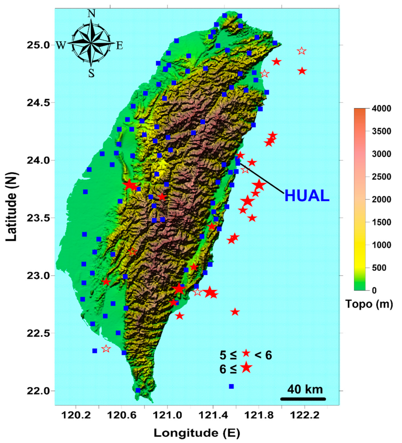
Figure 2.
Diagrams of displacements resulting from stress accumulation in homogeneous and inhomogeneous materials. When the same stress accumulates in homogeneous materials in (a), the quantity of displacements is associated with the Young’s modulus. In reality, because the surface crust is comprised of materials with different values of Young’s modulus, characteristics of stress (as shown by blue arrows) are misunderstood when only the quantity of displacements is taken into account. On the other hand, displacements resulting from stress accumulation exhibit a similar direction regardless of the Young’s modulus of materials (as shown by blue arrows) in inhomogeneous materials in (b). The direction of stress-inducing displacements is a good substitute for the quantity of the displacements and further approaches the intrinsic qualities of stress-inducing phenomena involving inhomogeneous structures.

Figure 3.
Eleven IMFs and the residual derived by HHT from decomposition of the east–west component of the GPS position of the HUAL station. (a) shows crustal displacements on the east-west component at the HUAL station. (b–l) are the IMF1-11. (m) is the residual obtained after the EMD process. MF denotes the median instantaneous frequency of each IMF.
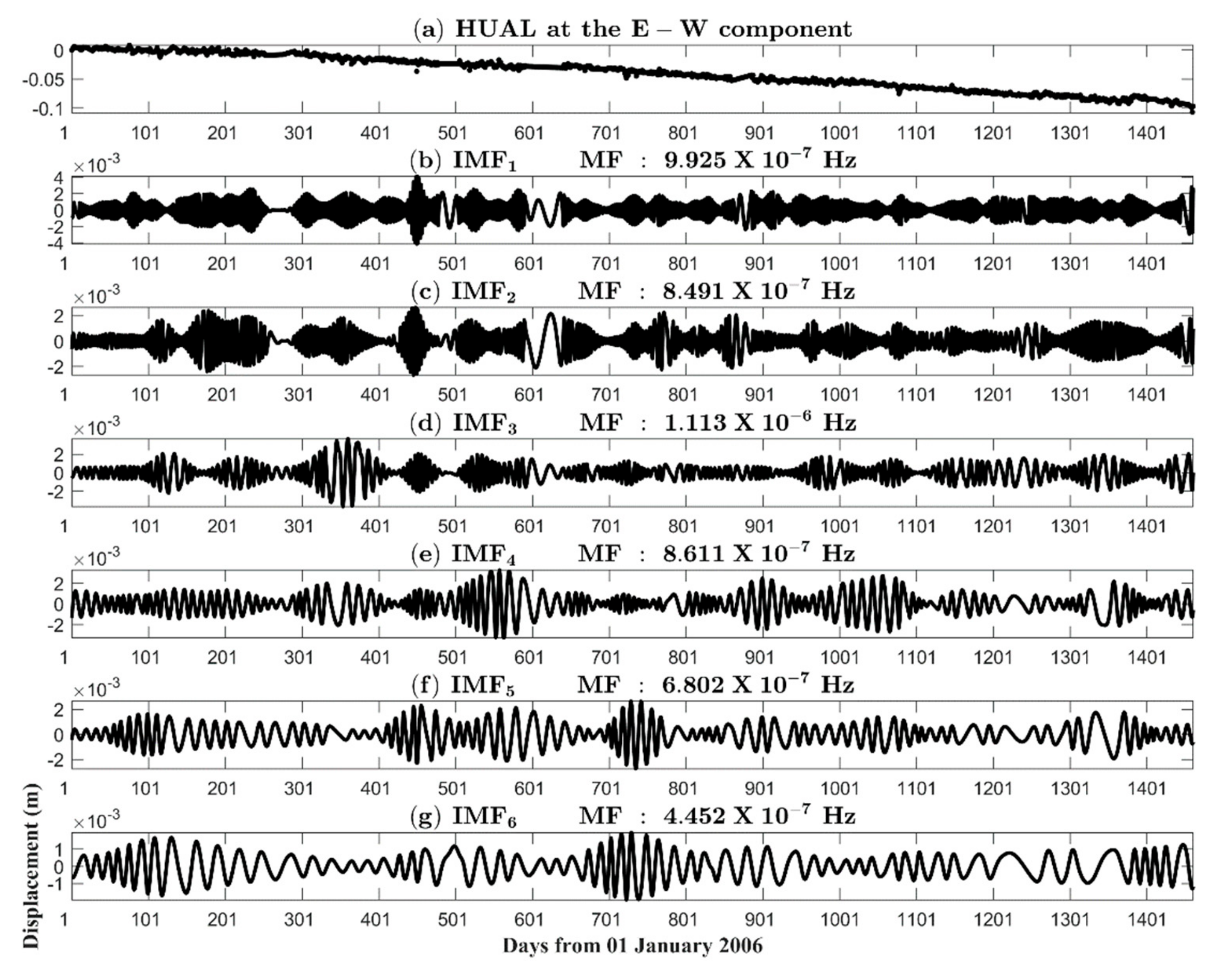
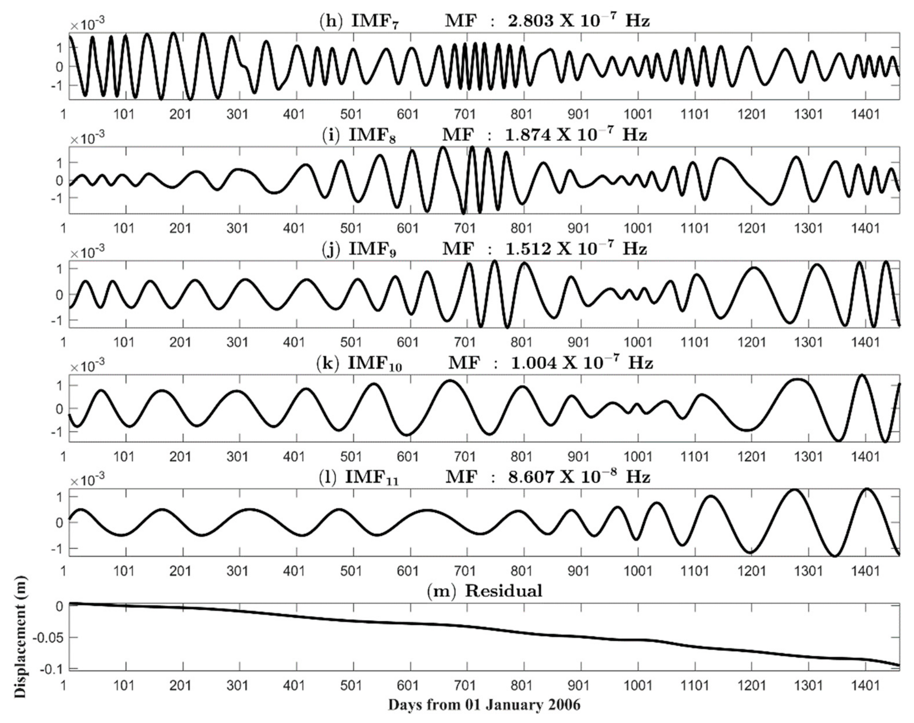
Figure 4.
The filtered deformation derived by the band pass filter for HUAL station. (a) exhibits the noise computed by using a high-pass filter of a frequency > 5.787 × 10⁻⁷ Hz. (b) shows the noise-free data. (c) reveals the variations of the long-term effects. (d) is the filtered displacements using a band-pass filter of a frequency band between 7.716 × 10⁻⁸ Hz and 5.787 × 10⁻⁷ Hz. The grey lines in (b) and (d) show the raw data.

Figure 5.
Maps of θw’ from 30 to 1 days before the earthquake day (EQD) in EQ28. The largest black star is the CWB-published epicenter of the EQ28. The blue crosses depict locations of the upper 0.5% θw’, indicating possible epicenters before EQ28 occurred. The pink and yellow colors denote areas of small (~0.011) and large (~0.02) θw’, respectively. Black arrows show the direction of surface deformation.

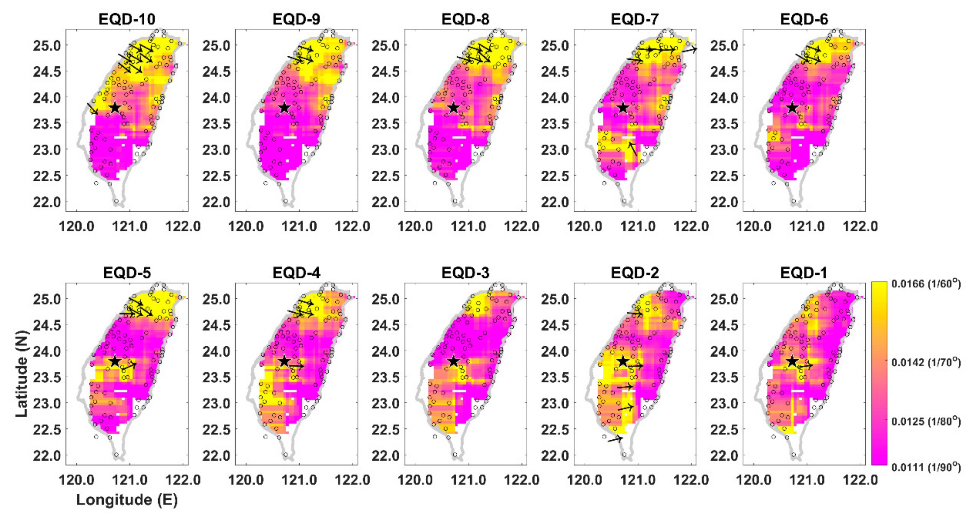
Figure 6.
The relationship between the P axis and θ(r, t) for the 32 studied earthquakes. Colors ranging from pink to yellow denote quantities of θ(r, t). If θ(r, t) > 0.0211, the black arrows are shown on the diagrams and their directions denote orientations of the GPS azimuths derived from the residual displacements. Notably, the value of 0.0211 is the so-call anomalous band (i.e., mean+2σ) computed from the inverse of the difference of the GPS azimuths between every pair of stations during the entire study period. The fault plane solution of each earthquake is shown in the upper right diagram. The P axis agreement (disagreement) with the aligned GPS azimuths is shown by using blue (black) color and marked above on associated days (below the fault plane solutions).

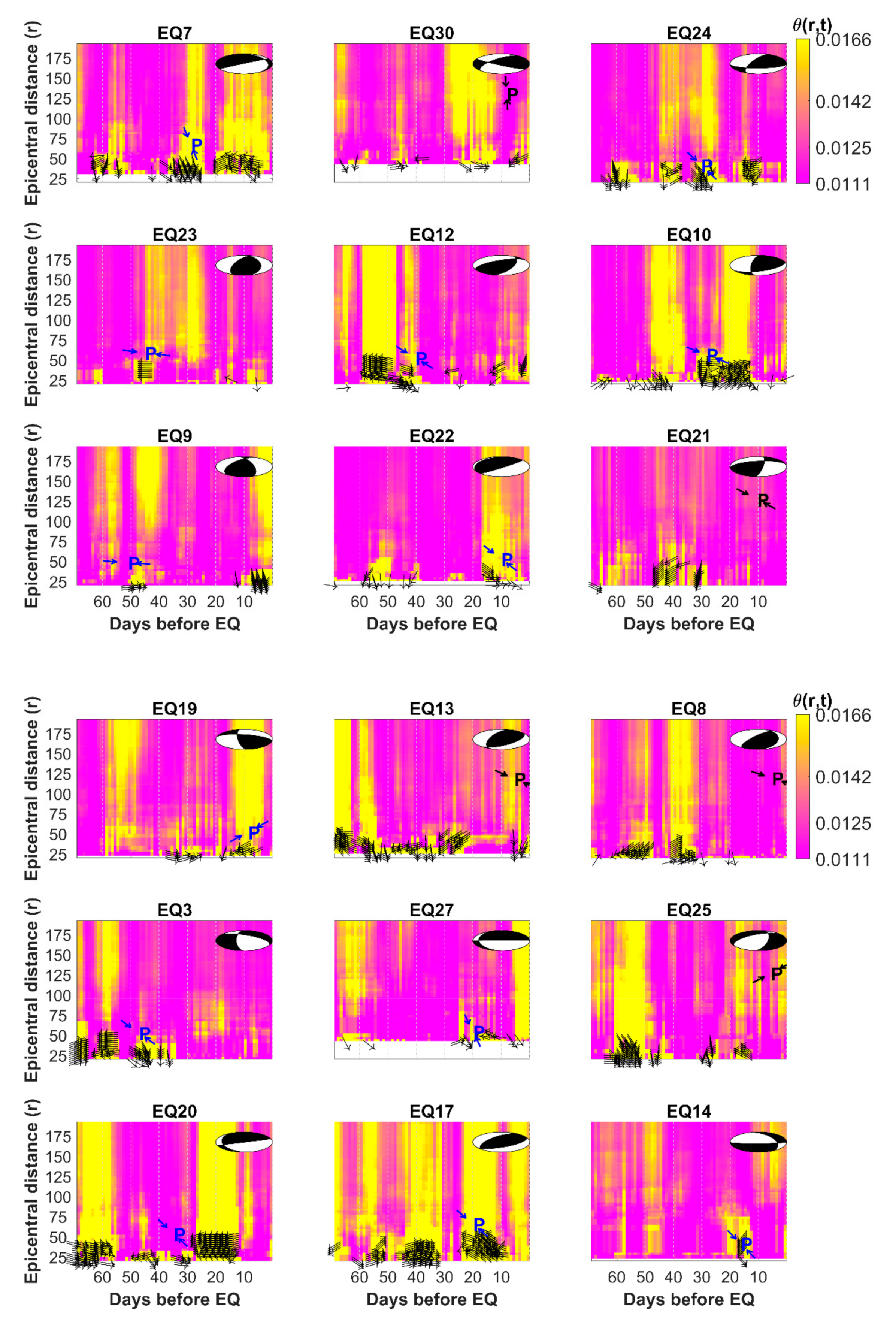
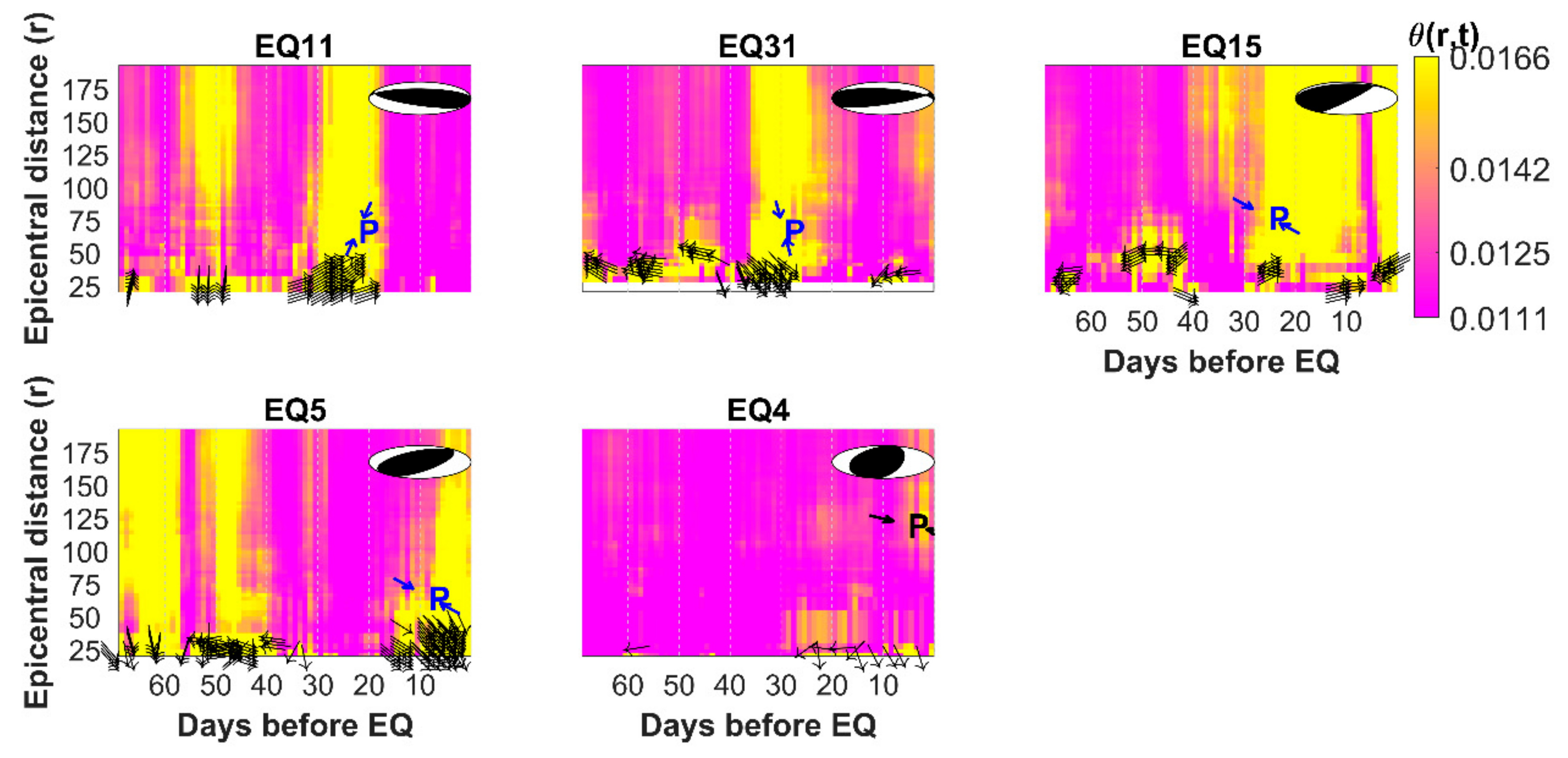
Figure 7.
Variations of θ(r, t) for 12 events sorted by earthquake magnitude. The red lines show θ(r, t), and the blue lines show the percentage of GPS stations with epicentral distance < r. The horizontal black lines indicate the anomalous band of 0.0211.
Figure 7.
Variations of θ(r, t) for 12 events sorted by earthquake magnitude. The red lines show θ(r, t), and the blue lines show the percentage of GPS stations with epicentral distance < r. The horizontal black lines indicate the anomalous band of 0.0211.
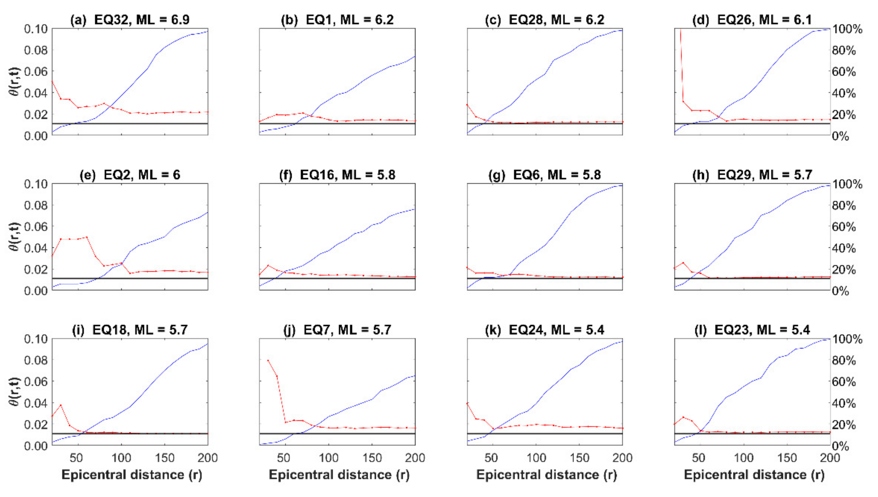
Figure 8.
Relationships between the maximum of θ(r, t), leading time, and earthquake magnitude. Relationships between the maximum of θ(r, t) and earthquake magnitude are shown in (a). In contrast, relationships between the leading time and earthquake magnitude are shown in (b). The black circles denote the 26 earthquakes detected during the study period. Note that the maximum of θ(r, t) and the leading time associated with the Tohoku-Oki and Chi-Chi earthquakes were computed using different r values (i.e., r ≠ 50 km) because the Tohoku-Oki earthquake occurred far away from the land and due to the relatively-low density GPS array surrounding the Chi-Chi earthquake in 1999.
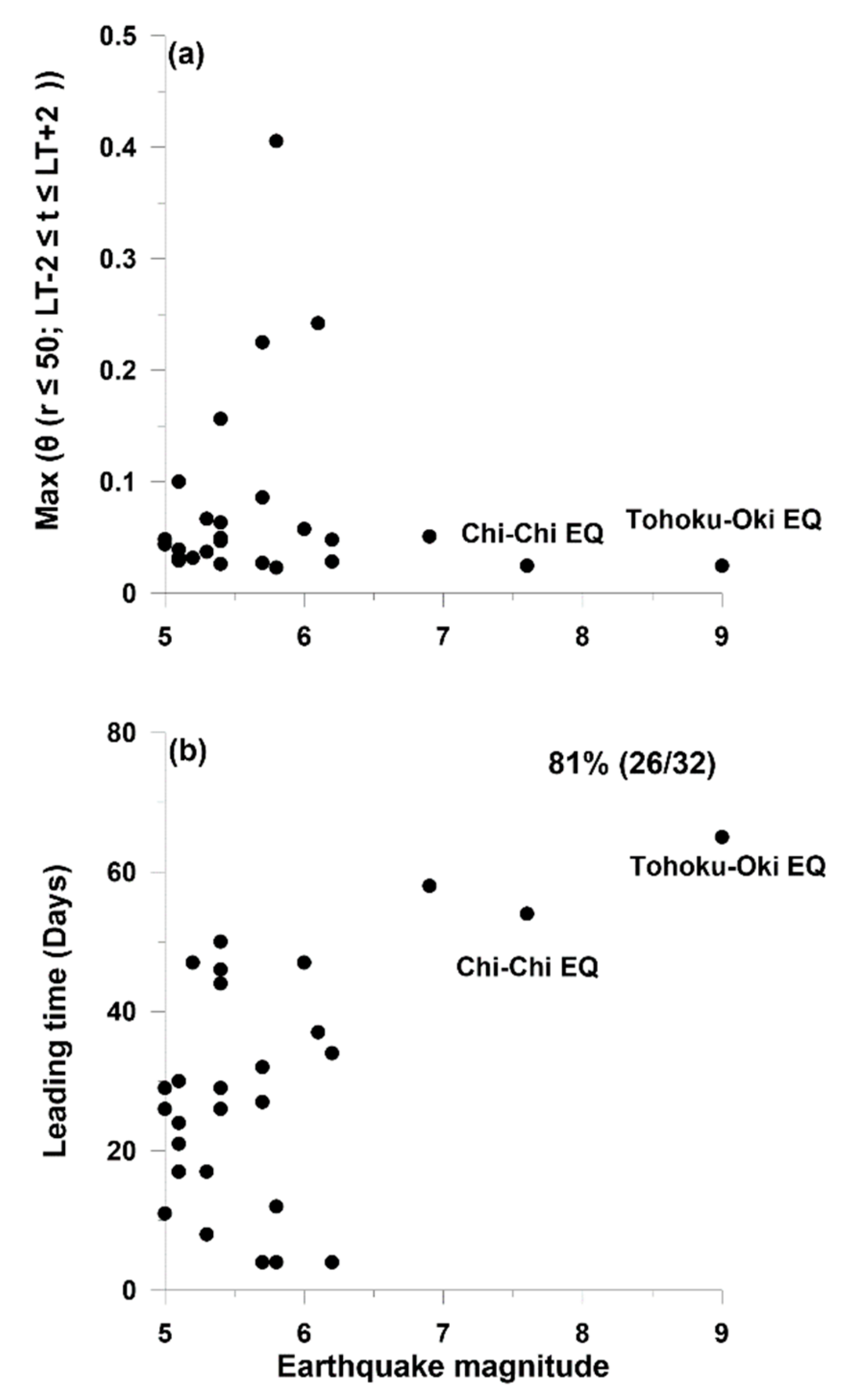
Figure 9.
Maps of θw from 30 to 1 days before the earthquake day (EQD) of EQ28. The largest black star is the CWB-published epicenter of the EQ28. The pink and yellow colors denote areas of small (~0.011) and large (~0.02) θw’, respectively. Black arrows show the direction of surface deformation.
Figure 9.
Maps of θw from 30 to 1 days before the earthquake day (EQD) of EQ28. The largest black star is the CWB-published epicenter of the EQ28. The pink and yellow colors denote areas of small (~0.011) and large (~0.02) θw’, respectively. Black arrows show the direction of surface deformation.
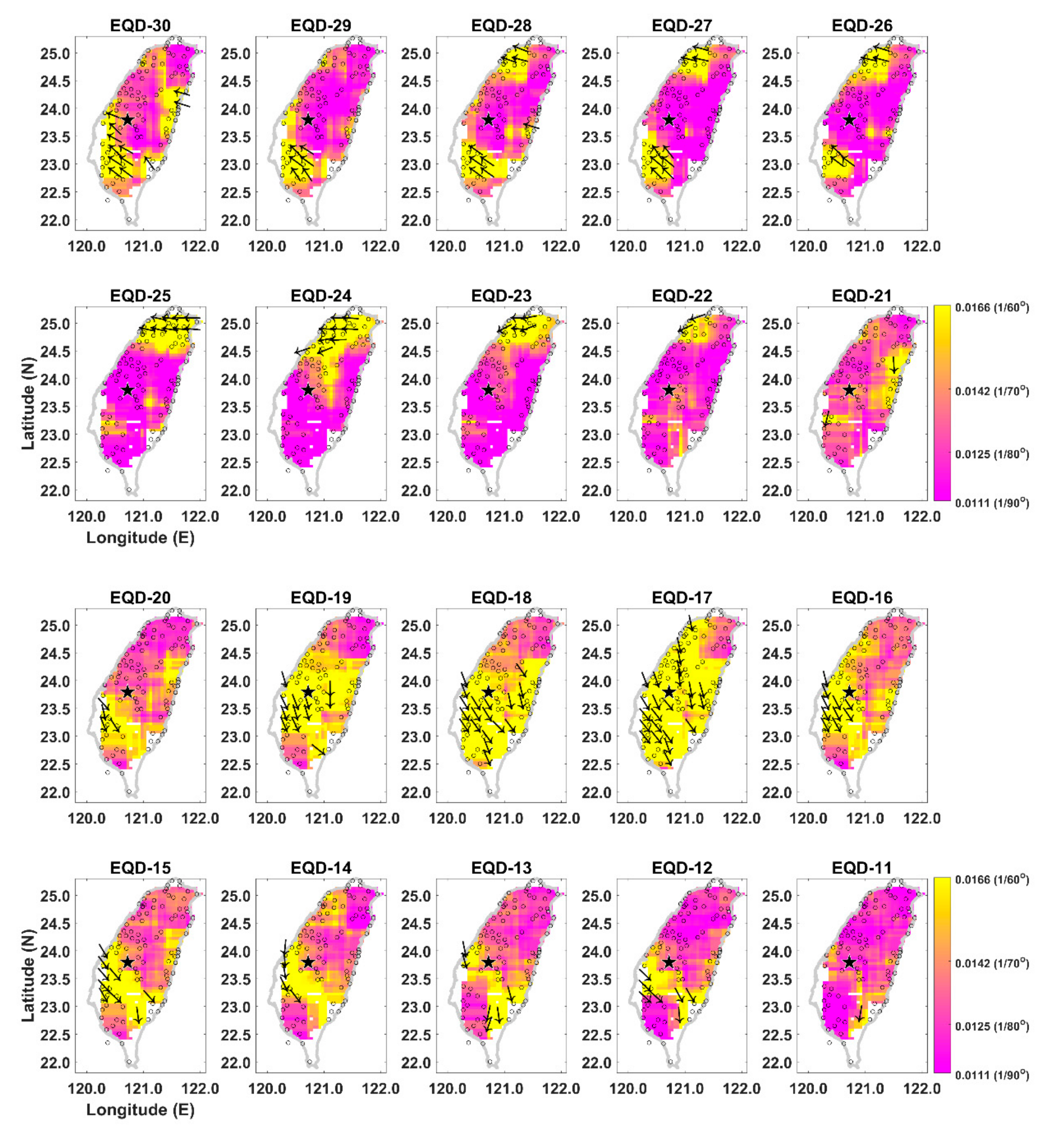
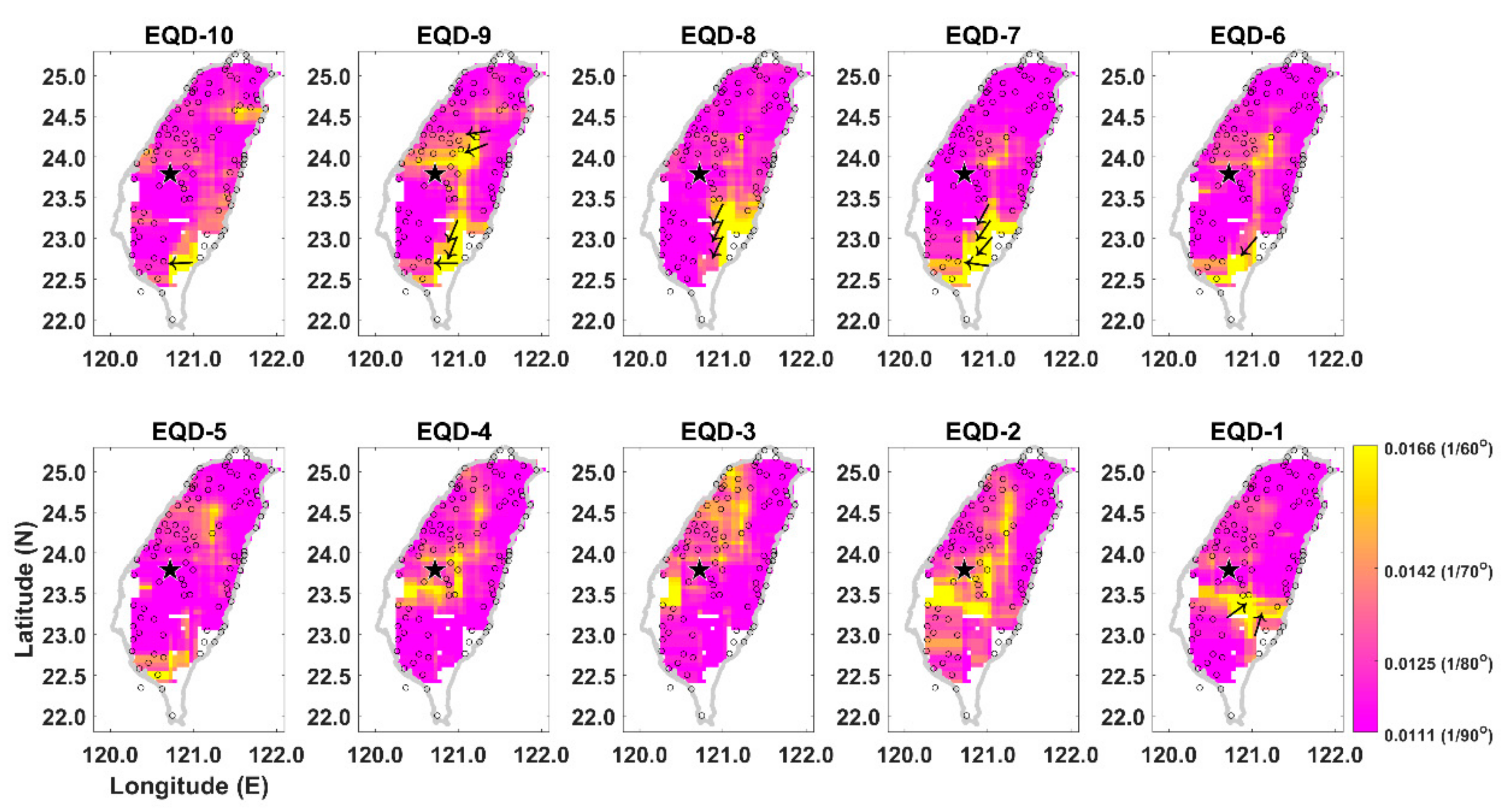
Figure 10.
Area skill scores for predictions with different lead times and alarm windows based on observations. We performed a forecasting experiment and predicted earthquakes with depths of less than 100 km and magnitude ≥ 5.0 during the studied period in and around Taiwan.
Figure 10.
Area skill scores for predictions with different lead times and alarm windows based on observations. We performed a forecasting experiment and predicted earthquakes with depths of less than 100 km and magnitude ≥ 5.0 during the studied period in and around Taiwan.
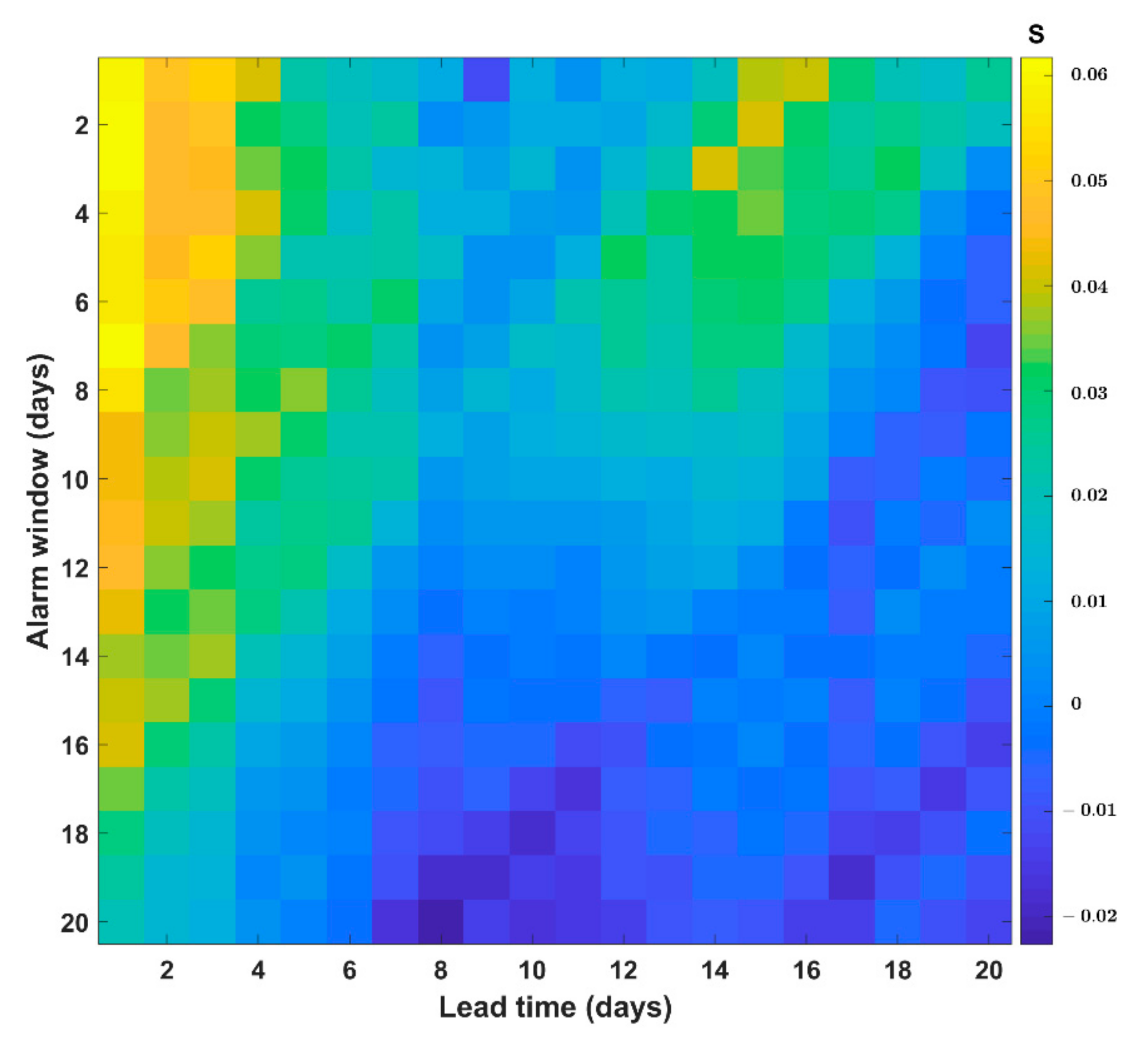
Figure 11.
The Molchan’s error diagram of the optimal prediction strategy based on the observations (lead time = 1 day and alarm window = 3 days).
Figure 11.
The Molchan’s error diagram of the optimal prediction strategy based on the observations (lead time = 1 day and alarm window = 3 days).


Table 1.
The 32 earthquakes (ML ≥ 5.0) that occurred in 2006–2009 and were used in this study. NaN denotes that a phase of stress loading was not detected. ID with * reveals earthquakes utilized in Figure 8. The LT is the leading time that reveals the time of aligned horizontal azimuths before the earthquakes. The strikes, dips, and slips are dislocation parameters of the faults.
| ID | Time | ML | Longitude (°) | Latitude (°) | θ | LT (Day) | Strike (°) | Dip (°) | Slip (°) | Direction of P axis (°) |
|---|---|---|---|---|---|---|---|---|---|---|
| 1 * | 2006-4-1 10:2:19.54 | 6.2 | 121.081 | 22.884 | 0.0478 | 34 | 193.6 | 58.9 | 30.2 | 141 |
| 2* | 2006-4-15 22:40:55.37 | 6 | 121.304 | 22.856 | 0.0575 | 47 | 214.6 | 46.7 | 116.4 | 106 |
| 3 | 2006-4-28 9:5:26.96 | 5.2 | 121.611 | 23.985 | 0.0316 | 47 | 300.0 | 42.0 | −141.5 | 135 |
| 4 | 2006-6-4 9:6:1.05 | 5 | 121.263 | 22.854 | NaN | NaN | 196.9 | 34.4 | 95.1 | 291 |
| 5 | 2007-7-16 23:42:52.18 | 5 | 121.545 | 23.57 | 0.0485 | 11 | 226.1 | 37.6 | 98.8 | 130 |
| 6 * | 2007-7-23 13:40:2.44 | 5.8 | 121.636 | 23.716 | 0.4056 | 12 | 26.1 | 38.0 | 89.9 | 301 |
| 7 * | 2007-8-9 0:55:47.36 | 5.7 | 121.085 | 22.65 | 0.0860 | 27 | 340.3 | 14.7 | −168.6 | 164 |
| 8 | 2007-10-11 3:5:1.7 | 5.2 | 121.85 | 24.749 | NaN | NaN | 7.4 | 27.1 | 66.5 | 295 |
| 9 | 2007-10-17 14:40:0.03 | 5.4 | 121.612 | 23.501 | 0.0470 | 50 | 210.2 | 41.2 | 125.8 | 95 |
| 10 | 2007-11-28 21:5:13.72 | 5.4 | 121.976 | 24.781 | 0.0637 | 26 | 63.7 | 39.1 | 141.6 | 299 |
| 11 | 2007-12-5 1:41:42.53 | 5.1 | 121.187 | 23.075 | 0.0298 | 24 | 272.3 | 38.5 | 69.7 | 197 |
| 12 | 2008-2-17 20:33:2.32 | 5.4 | 121.461 | 23.307 | 0.1566 | 44 | 240.4 | 47.3 | 119.0 | 130 |
| 13 | 2008-3-4 17:31:47.48 | 5.2 | 120.696 | 23.207 | NaN | NaN | 46.3 | 41.9 | 110.8 | 302 |
| 14 | 2008-4-14 15:39:44.45 | 5.1 | 121.333 | 22.834 | 0.0292 | 17 | 337.9 | 33.9 | −24.8 | 325 |
| 15 | 2008-5-13 18:27:55.34 | 5 | 121.041 | 22.766 | 0.0441 | 26 | 252.8 | 12.6 | 129.6 | 129 |
| 16 * | 2008-6-1 16:59:23.74 | 5.8 | 121.79 | 24.861 | 0.0232 | 4 | 55.2 | 24.2 | 73.4 | 338 |
| 17 | 2008-8-1 18:55:49.32 | 5.1 | 121.526 | 24.048 | 0.1000 | 17 | 219.4 | 44.7 | 75.0 | 140 |
| 18 * | 2008-12-2 3:16:54.23 | 5.7 | 121.486 | 23.338 | 0.2251 | 32 | 232.8 | 42.7 | 126.7 | 118 |
| 19 | 2008-12-23 0:4:43.82 | 5.3 | 120.551 | 22.946 | 0.0371 | 8 | 282.4 | 47.9 | 27.0 | 233 |
| 20 | 2009-1-3 22:4:34.97 | 5.1 | 121.733 | 24.154 | 0.0393 | 30 | 165.5 | 20.3 | 4.4 | 143 |
| 21 | 2009-4-17 12:37:48.89 | 5.3 | 121.682 | 23.917 | NaN | NaN | 260.0 | 40.7 | 156.5 | 126 |
| 22 | 2009-6-28 9:34:56.19 | 5.3 | 121.753 | 24.182 | 0.0667 | 17 | 217.6 | 9.1 | 79.3 | 137 |
| 23 * | 2009-7-26 1:0:12.37 | 5.4 | 120.957 | 23.685 | 0.0262 | 46 | 356.6 | 36.8 | 72.1 | 279 |
| 24 * | 2009-7-26 6:10:59.79 | 5.4 | 121.318 | 23.429 | 0.0497 | 29 | 88.9 | 51.4 | 145.6 | 323 |
| 25 | 2009-8-21 20:57:44.74 | 5.1 | 120.464 | 22.364 | NaN | NaN | 232.5 | 38.5 | −54.0 | 234 |
| 26 * | 2009-10-3 17:36:6.28 | 6.1 | 121.579 | 23.648 | 0.2423 | 37 | 269.6 | 44.4 | 174.9 | 127 |
| 27 | 2009-10-22 23:5:5.13 | 5.1 | 121.488 | 22.685 | 0.0324 | 21 | 172.4 | 19.2 | −7.5 | 161 |
| 28 * | 2009-11-5 9:32:57.66 | 6.2 | 120.719 | 23.789 | 0.0286 | 4 | 228.1 | 59.0 | 150.9 | 100 |
| 29* | 2009-11-5 11:34:21.26 | 5.7 | 120.755 | 23.769 | 0.0273 | 4 | 213.0 | 48.6 | 134.4 | 93 |
| 30 | 2009-11-15 14:47:49.14 | 5.5 | 122.174 | 24.946 | NaN | NaN | 221.8 | 49.6 | 15.9 | 177 |
| 31 | 2009-11-21 17:27:51.26 | 5 | 121.762 | 24.222 | 0.0439 | 29 | 282.8 | 38.5 | 122.4 | 170 |
| 32 * | 2009-12-19 13:2:16.34 | 6.9 | 121.663 | 23.788 | 0.0510 | 58 | 260.0 | 32.1 | 175.1 | 111 |
Table 2.
Median frequency and period for the 11 IMFs shown in Figure 2.
Table 2.
Median frequency and period for the 11 IMFs shown in Figure 2.
| IMFs | Median Frequency (Hz) | Median Period (days) |
|---|---|---|
| 1 | 9.9249 × 10⁻⁷ | 11.7 |
| 2 | 8.4907 × 10⁻⁷ | 13.6 |
| 3 | 1.1127 × 10⁻⁶ | 10.4 |
| 4 | 8.6112 × 10⁻⁷ | 13.4 |
| 5 | 6.8018 × 10⁻⁷ | 17.1 |
| 6 | 4.4520 × 10⁻⁷ | 26.0 |
| 7 | 2.8028 × 10⁻⁷ | 41.3 |
| 8 | 1.8737 × 10⁻⁷ | 61.8 |
| 9 | 1.5120 × 10⁻⁷ | 76.5 |
| 10 | 1.0041 × 10⁻⁷ | 115.3 |
| 11 | 8.6075 × 10⁻⁸ | 134.5 |
© 2020 by the authors. Licensee MDPI, Basel, Switzerland. This article is an open access article distributed under the terms and conditions of the Creative Commons Attribution (CC BY) license (http://creativecommons.org/licenses/by/4.0/).
Share and Cite
MDPI and ACS Style
Chen, C.-H.; Yeh, T.-K.; Wen, S.; Meng, G.; Han, P.; Tang, C.-C.; Liu, J.-Y.; Wang, C.-H. Unique Pre-Earthquake Deformation Patterns in the Spatial Domains from GPS in Taiwan. Remote Sens. 2020, 12, 366. https://doi.org/10.3390/rs12030366
AMA Style
Chen C-H, Yeh T-K, Wen S, Meng G, Han P, Tang C-C, Liu J-Y, Wang C-H. Unique Pre-Earthquake Deformation Patterns in the Spatial Domains from GPS in Taiwan. Remote Sensing. 2020; 12(3):366. https://doi.org/10.3390/rs12030366
Chicago/Turabian StyleChen, Chieh-Hung, Ta-Kang Yeh, Strong Wen, Guojie Meng, Peng Han, Chi-Chia Tang, Jann-Yenq Liu, and Chung-Ho Wang. 2020. "Unique Pre-Earthquake Deformation Patterns in the Spatial Domains from GPS in Taiwan" Remote Sensing 12, no. 3: 366. https://doi.org/10.3390/rs12030366
Note that from the first issue of 2016, this journal uses article numbers instead of page numbers. See further details here.