Estimation of Ice Thickness and the Features of Subglacial Media Detected by Ground Penetrating Radar at the Baishui River Glacier No. 1 in Mt. Yulong, China

Abstract

Using ground-penetrating radar (GPR), we measured and estimated the ice thickness of the Baishui River Glacier No. 1 of Yulong Snow Mountain. According to the position of the reflected media from the GPR image, combined with the radar waveform amplitude and polarity change information, the ice thickness and the changing medium position at the bottom of this temperate glacier were identified. Water paths were found in the measured ice, including ice caves and crevasses. A debris-rich ice layer was found at the bottom of the glacier, which produces strong abrasion and ploughing action at the bedrock surface. This results in the formation of different detrital layers stagnated at the ice-bedrock interface and numerous crevasses on the bedrock surface. Based on the obtained ice thickness and differential GPS data, combined with Landsat images, the kriging interpolation method was used to obtain grid data. The average ice thickness was 52.48 m and between 4740 and 4890 m above sea level, with a maximum depth of 92.83 m. The bedrock topography map of this area was drawn using digital elevation model from the Shuttle Radar Topography Mission. The central part of the glacier was characterized by small ice basins with distributed ice steps and ice ridges at the upper and lower parts.

1. Introduction

Ground penetrating radar (GPR) is a type of equipment that uses a continuous electromagnetic pulse to visualize shallow geological structures. As there are different dielectric constants from different substances, the distribution or depth of the specific substance can be identified and analyzed according to the image from GPR, for instance, ice cavities, subglacial debris, and bedrock [1]. Due to the low attenuation rate and strong penetrability of GPR electromagnetic wave propagation in glacier medium, the GPR detection technology is widely used in the research area of ice thickness and subglacial terrains.

In particular, data of ice thickness has been obtained from polar glaciers in western China and has played an important role in the research of global changes [2,3,4,5,6,7,8,9,10,11,12,13,14,15]. However, due to the higher ice temperature and water content as well as the high attenuation rate of the GPR electromagnetic signal in temperate glaciers, the penetrability in temperate ice can rapidly decrease. The higher the water content is, the stronger wave attenuation and scattering are. These problems increase the difficulty of GPR employed in temperate glaciers [16]. In addition, the reflection of electromagnetic waves from bedrock also experiences interference and significantly influences the interpretation of GPR images [17].

The ice thickness can be measured in some temperate and multi-thermal glaciers through electromagnetic wave filtering technology using a reasonable interpretation with low-frequency-monopulse GPR. Measurements and studies showed that the scattering rate of electromagnetic waves in temperate glaciers is significantly reduced as the radar frequencies vary between 10 and 25 Mhz [18,19,20]. The phase polarity of electromagnetic waves changes between interfaces of different subglacial media [21]. As the water content varies in different depths of temperate glaciers, the propagation speeds of electromagnetic waves in ice are also different [18]. The discontinuous electromagnetic waves may result from radio wave diffraction generated at the interface between ice and bedrock with lower energy, or may be caused by the presence of subglacial channels [20].

At present, there are few measurements and ice thickness studies for temperate glaciers in China. The B-1 ground-penetrating ice radar was applied by the Qinghai-Tibet Plateau (QTP) Scientific Investigation Team organized by the Chinese Academy of Sciences in 1983 when the ice tongue sections of four temperate glaciers in Gongga Mountain were measured. The average thickness of the transverse section within 2–3 km from the ice tongue terminal on each glacier was 100–120 m [22,23]. In 1990, the thickness of Hailuogou glacier was measured by GPR, and the average ice thickness at 3096–3150 m above sea level (a.s.l.) was from 49.2 to 52.9 m, with the maximum ice thickness between 58.5 and 75.6 m [24]. In 2007, a new ground-penetrating radar with an antenna frequency of 100 MHz was used to measure the ice thickness on the right branch of the Paron No. 12 glacier in the Gangrigabu region, southeast of the QTP, with an area of 0.95 km² and a length of 1.8 km. The thickest part at the ice tongue of 5100 m a.s.l. was about 40 m thick [25].

Under the influence of climate warming, a typical monsoon temperate glacier in Yulong Snow Mountain (Mt. Yulong) located in the southernmost part of China, has been continuously shrinking at a faster rate, and this has resulted in a dense distribution of crevasses on its surface [26,27,28,29]. These drastic changes of glaciers have exerted a great impact on the local social economy, especially on the tourism industry and the living conditions of the local residents in Lijiang [30]. The intensification of glacier melting also led to a resource reduction of regional water and glacier tourism, and the occurrence of some geological disasters [31,32].

The calculation of the reserve of each glacier in Mt. Yulong from two-time inventories of Chinese glaciers [33,34] was based on the empirical formula of the glacier’s volume and area. The accuracy of glacier reserve estimation can be greatly improved through the ice thickness measurements. Unfortunately, due to the high water content of the ice, the ice thickness in this area has been rarely measured. Apart from in 1982, the measurements of glacier thickness with different types of the GPR (personal communication) were conducted only in 2011 and 2014; however, a clear ice-bedrock interface was not detected. Although ice thickness estimation on this glacier is still a difficult task, the aims of our work are a detailed interpretation and estimation of the ice thickness and its spatial distribution, the identification of subglacial media, and analysis of the bedrock topography of the glacier, based on the measured data by GPR and GPS.

2. Materials and Methods

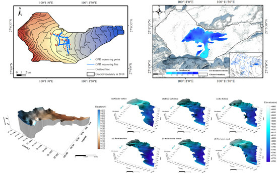
2.1. Study Area

Mt. Yulong (27°10′–27°40′ N, 100°9′–100°20′ E) is located in the subtropical zone of low latitude, the southeast edge of the QTP, and the southern end of the Hengduan Mountains (Figure 1), 25 km north of Lijiang City, Yunnan Province, which is the closest glacier to the Equator [35]. Mt. Yulong is 35 km long from north to south, and 13 km wide from east to west, with the highest peak (Shanzidou) at 5596 m a.s.l. The unique geographical location and glacial tourism resource makes it a famous tourist destination in China [36]. The existing glaciers extend over 4350 m a.s.l. in Mt. Yulong, the vestiges formed during the Last Ice Age and previous glaciation extend between 3000 and 4000 m a.s.l. There is a large area of glacial sediments on the eastern slope of Mt. Yulong between 2800 and 3500 m a.s.l. [37].

According to the Glacier Inventory of the Yangtze River Basin in 1982 [33], there were 19 existing glaciers with a total area of 11.61 km², including 15 in the east and 4 in the west. The Baishui River No. 1 Glacier (BRG1) located in the eastern slope and terminated at 4100 m, is the largest glacier, with a length of 2.7 km and an area of 1.52 km². In recent decades, the glaciers on Mt. Yulong have retreated rapidly, and there only were 13 modern glaciers in 2009: 11 on the eastern slope and 2 on the western slope, with a total area of 4.97 km², among which the BRG1 had an area of 1.44 km² and terminated at 4415.4 m a.s.l. [34]. From 1957 to 2009, the annual change rate of glacier area was −1.19%, which is much higher than the other regions in China [27]. By 2017, the Mt. Yulong had 13 glaciers with an area of 4.48 km², among which the BRG1 had reduced its length to 1.9 km and area to 1.32 km², and the glacier ended at 4395 m a.s.l. [29].

Mt. Yulong is jointly influenced by the climate of the southwest, southeast, and Tibetan plateau monsoons in different seasons. According to the snow pit profile and measured meteorological data at different elevations in the glacier area, the precipitation near the original snow line (4800 m a.s.l.) is 2400–3100 mm and average annual temperature of −1.5 to −2.3 °C from 4800 to 5000 m a.s.l. in 2011, in comparison with that of −3.3 to −4.7 °C in 1982, indicating an obviously warming in this area [38].

2.2. Data

2.2.1. Field Observation Data

The ice thickness of the BRG1 was measured with GPR (pulse EKKOPRO100A) in 2018, and a shielded antenna with a central frequency of 100 MHz and omni-directional antenna emission were selected. The position data were detected using GPS (TrimbleGeoXT6000) along the GPR measuring paths (Figure 2a), with a vertical error and horizontal error of 1 cm ± 2 ppm. The GPR transmitting and receiving antenna were moved synchronously along the measuring line at a 4 m distance, and the measuring point was located in the middle between two antennas [4,5].

There were intensive crevasses on the glacier tongue between 4400 and 4500 m a.s.l. (Figure 2b). As underlying bedrock topography has an influence on glacier movement, the glacier was divided into a north and south part by a surface moraine in the middle, where the glacier was narrower. There are some deep ice crevasses through the glacier between 4600 and 4700 m a.s.l. (Figure 2c,d). In the upper part of the glacier (firn basin) above 4700 m a.s.l., the ice surface was relatively flat [39]. Therefore, the relatively flat area at 4780–4830 m a.s.l. was selected for the measurement of the ice thickness (Figure 2e).

Last, three transverse profiles perpendicular to the glacier’s horizontal midstream and three longitudinal profiles parallel to the middle line were established as follows: (1) Profile L1 at 4780–4793 m a.s.l. from south to north. The measuring point A in profile L1 is a subglacial layer interpretation sample of a single waveform track. (2) Profile L3 at 4774–4800 m a.s.l. from south to north, located in the lower part of the original glacier accumulation area (OGAA). The points C, D and E in profile L3 are the abnormal points. (3) Profile L5 at 4806–4847 m a.s.l. from north to south, located in the upper part of the OGAA. (4) The shorter profile T2 at 4792–4800 m a.s.l. from east to west, close to the glacier flowline and located in the central of the OGAA. The measuring point B in profile T2 is a subglacial layer interpretation sample of a single waveform track. (5) Profile T4 at 4790–4831 m a.s.l. from east to west, located in the north of the OGAA. The points F, G, H, I, and J in profile T4 are the abnormal points. (6) Profile T6 at 4807–4782 m a.s.l. from west to east, located in the south of the OGAA.

The GPR measuring network included the boundary and central part of the OGAA; however, certain survey lines did not reach the glacier’s edge, due to the existence of large crevasses or deep snow cover there, making it difficult to carry out the survey work. During the survey period, the work field was free of snow.

2.2.2. Image Data

The main image sources were Landsat ETM+/OLI (band 5\4\3; band 6\5\4) from the United States Geological Survey (USGS, https://ers.cr.usgs.gov/), and were orthorectified automatically by USGS using a digital elevation model from the Shuttle Radar Topography Mission (SRTM DEM). The LocalSpaceViewer software was used to download Pléiade satellite images provided by Google Earth, with a spatial resolution of 1.2 m (corresponding to 17 levels of resolution). The selected scenes were acquired in 2018 without clouds or seasonal snow. The nominal vertical accuracy of the SRTM DEM (the fourth version) is 6 m, relatively, and 16 m, absolutely, and the nominal horizontal accuracy is 15 m, relatively, and 20 m, absolutely [13].

The geodetic reference for SRTM DEM is the World Geodetic System 1984 (WGS84). The topography map at scales of 1:50,000 were derived from aerial photographs in 1957 provided by the Northwest Institute of Eco-Environment and Resources, Chinese Academy of Sciences. The First Glacier Inventory Dataset of China (1956–1983) and the Second Glacier Inventory Dataset of China Version 1.0 (2006–2010) were provided by the Cold and Arid Region Scientific Data Center (http://data.casnw.net) [34].

2.3. Methods

2.3.1. Method of GPR Measurement Data Interpretation

Images of thickness measured by radar are typically recorded in the form of pulse waves. The positive and negative peaks of the waveform are represented, respectively, by black and white, or by gray scale and color. In this way, the ice-rock interface and its fluctuations can be vividly represented by the same phase axis or equal gray scale and equal color line [4,5]. However, due to the strong melting of the glacier in summer, the rapid movement causes the ice body to break and melted water to penetrate into the ice and even down to the bottom, forming drainage paths and permeable holes inside the glacier. Thus, when a high-frequency modulated pulse is used to detect the ice, this may cause complex echoes [23].

With the temperature of glacier ice at the melting point in summer, the liquid water in the ice pores can interfere with the electromagnetic waves and cause diffraction. Intense scattering occurs within the transition layer between the ice, subglacial sediments, and bedrock, due to the inclusion of small amounts of water [16]. Therefore, temperate ice with electromagnetic wave creates scatter by numerous stacks of small hyperbolas, which is different from the relatively transparent reflection of cold ice [40]. The energy of the electromagnetic wave is attenuated and greatly decreases when it penetrates ice with melting water that reaches the bottom of the glacier. The bedrock in Mt. Yulong is limestone, and a large amount of debris is produced under glacial erosion, and prone to dissolution by meltwater at the glacier bottom [23]. All these factors affect the electromagnetic wave reflection of the bedrock in the GPR images, and therefore the ice-bedrock interface in temperate glaciers is difficult to identify.

Observations found that there is often a layer of debris-rich ice up to several meters thick at the base of a temperate glacier. Between the glacier bottom and the bedrock, there exists a water-saturated sand and gravel layer, which is partially or completely ice-free, suggesting that the theoretical assumption of a clear interface between the ice and bedrock is incorrect [16]. Aditya et al. [17] used GPR to measure the ice thickness of the melting zone in Satopanth glacier in the central Himalayas, with GPR antenna frequencies of 16 MHz, 20 MHz, and 80 MHz. However, only two relatively clear bedrock interfaces in 25 profiles were obtained, suggesting a clear ice-bedrock interface, which is difficult to obtain in the temperate glacier by GPR detection even with a lower frequency radar antenna.

Florence et al. [41] proposed an automatic GPR detection method to measure the thickness of temperate glaciers. Based on the level of the received energy and on the slope of the attenuation function over time, the method calculates the smallest root mean square of these two parameters on each trace, and compares this to the determined threshold of noise statistics. The assumption is that the glacier bottom is detected when the level and slope values are below the threshold. The results of the data analysis were roughly consistent with those obtained using the seismic and borehole methods.

Using the GPR data processing method proposed by Florence et al. [41], the GPR measurement raw data were processed using EKKO View Deluxe and ReflexW 5.0. The main processing sequences included: (1) zero correction to reset the time to zero when the signal was first sent; (2) Dewow (user’s guide of the software) to suppress low-frequency energy emitted by the field near the transmitter, which acts on each trace independently; (3) a Butterworth bandpass filter set the frequency spectrum below and above a filter band to zero, which was set the optimal frequency range between 25 and 180 MHz; (4) automatic gain control (AGC) was applied to strengthen the signals with depth [18,19,20,21,40,41,42]. However, there was still no continuous clear ice-bedrock interface in the GPR data processing results.

The reflection coefficient R of electromagnetic wave was calculated using the equation:

$$R=\frac{\sqrt{{\mathsf{\epsilon }}_1}-\sqrt{{\mathsf{\epsilon }}_2}}{\sqrt{{\mathsf{\epsilon }}_1}+\sqrt{{\mathsf{\epsilon }}_2}}$$

(1)

where ɛ₁ and ε₂ are dielectric constants of two different media. It can be seen from the equation above that the greater the difference of the two dielectric constants is, the larger the absolute value of the reflection coefficient [43]. The relative dielectric constants of common media in temperate glaciers include ice (ɛ = 4), air (ɛ = 1), water (ɛ = 80), and limestone (ɛ = 7–9). An electromagnetic wave enters two different medias in different orders, which causes not only the amplitude of the reflection coefficient R to change, but also the polarity (positive and negative) to change in reference to the characteristics of the reflection source waveform. According to Equation (1), positive and negative phase polarity changes of the radar wave respond to a sudden change of the dielectric constant from high to low, when the radar wave propagates at the interface position of different media. Therefore, the subglacial different media interface position can be determined by analyzing the radar waveform image [1,21].

There are snow, ice, ice meltwater, subglacial sediments, and subglacial channels and crevasses inside the glacier [16,23]. As the meltwater content and the dielectric constant between different subglacial media layers vary with depth, the intensity of the generated radar reflected wave is different, and, thus, the amplitude and phase polarity also change [1]. The GPR profile shows a wide distribution of electromagnetic wave energy, and the reflected energy continuously decreases with time. Each trace signal disappears at a different given time. The inconsistency of the meltwater content in ice may result in inhomogeneous layering within the ice and different attenuation degrees of the electromagnetic wave, which will cause part reflections on different traces and show discontinuity of the electromagnetic properties after the energy incident. Due to this, the bedrock layer exhibits heterogeneity in GPR images. The energy change is proposed to correspond to the reflection inside the ice, while the small change in the reflection wave energy corresponds to the part below the bedrock [41].

In summary, although the meltwater in temperate ice can largely absorb electromagnetic waves, the strength change image of the radar reflection wave at different depths can display the reflection intensity of the medium layer at different vertical positions. According to the amplitude and polarity changes of the radar reflection wave at corresponding locations, even though there is moraine debris or pellicular water between the glacier bottom and bedrock interface [16], the subglacial medium and the bedrock interface can be identified and analyzed [1,3,23]. Based on the GPR measurement profiles of the BRG1, the amplitude and polarity changes of each measured trace were analyzed in this study, and the subglacial media changes were indicated by characteristic signals. Therefore, this method is a feasible solution to the difficulties of obtaining the thickness data in temperate glaciers.

2.3.2. Method of Glacier Thickness Calculation

In the GPR image, the ice thickness was calculated using the two-way travel time of radar waves in the vertical direction [4,5] as an equation:

$$H=\frac{\sqrt{V^2{T}^2-X^2}}{2}$$

(2)

where H is the ice thickness, T is the two-way travel time of the radar wave, X is the distance between the antenna transmitting and receiving unit, and V is the propagation velocity of the radar wave in ice.

The ε of pure ice is 3.2; however, free liquid water in ice can cause ε to be greater than 3.2. As shown in

Table 1. Descriptive statistics in the electromagnetic wave propagation velocity variation with the meltwater content of temperate glaciers.

Temperate Glacier	Location	Meltwater Content in Temperate Glacier	Electromagnetic Wave Propagation Velocity
Satopanth glacier [17]	Central Himalayas	-	0.156 ± 0.008 m/ns
Falljӧkull glacier [18]	Southeast of Iceland	0.23–0.34%	0.166 m/ns
		3–4.1%	0.149 m/ns
		2.4–3%	0.152 m/ns
		0.09–0.14%	0.167 m/ns
Johnsons Glacier [20]	Livingston Island, South Shetland Islands, Antarctica	0.4–2.3%	0.157–0.166 m/ns
Mont-de-Lans glacier [41]	Western of the Alps	0%	0.168 m/ns
		1%	0.150 m/ns
		5%	0.138 m/ns
Tasman and Mueller glaciers [45]	Alps in the southern New Zealand	-	0.159 m/ns

, the electromagnetic wave propagation velocity of temperate glaciers decreases with the increase of meltwater in ice, which varies at different depths [17,18,20,21,41,44]. As there are many crevasses on the glacier surface, the common midpoint method was not used to measure the electromagnetic wave speed. According to the above presented results, we took 0.156 m/ns as an average speed of the electromagnetic wave at BRG1, and the ice thickness was calculated using Equation (2).

To identify the correct reflection layer at the glacier bottom and the bedrock interface, some of the GPR data were not interpreted, due to strong diffraction of the reflected waves or measuring points without obvious amplitude and polarity changes. In addition to the systematic errors of the measurement data, the internal physical characteristics of the glacier also caused errors. The density and conductivity of ice vary with water content and depth. There are many ice caves inside the glacier, which caused a strong electromagnetic wave echo, as well as diffraction and scattering, so that the radar waves appeared as multiple reflections inside the ice, causing errors in the interpretation of the ice thickness at certain measuring points. Therefore, the relative error of GPR measurement should be calculated.

The propagation velocity of radar electromagnetic wave in cold glacier is between 0.167 and 0.171 m/ns. According to the calculation of Sun et al. [4], the maximum relative error of GPR measurement in cold glacier is 1.18%. However, the electromagnetic wave propagation velocity in temperate glaciers range from 0.138 to 0.168 m/ns (Table 1), which is lower than that in cold glaciers, with the difference of meltwater content from the glacier surface to bottom. In this study, the average velocity of 0.156 m/ns was adopted, which may overestimate the ice thickness. The relative error of ice thickness by the GPR measurement was based on the following equation [4,5]:

$$\frac{dh}{h}=\frac{dv}{2v}$$

(3)

where v is the propagation velocity of an electromagnetic wave in the subglacial medium (m/ns), and h is the thickness of the glacier (m). The maximum relative error of ice thickness in this work was 9.62%.

2.3.3. Method of Glacier Thickness Interpolation

To analyze the spatial distribution characteristics of the ice thickness, the boundary of the glacier must first be determined. The Landsat images were used to acquire the glacier boundary in 2018. All the images were projected in UTM zone 47N. The data processing steps are as follows: (1) the ENVI plugin tm_destripe was used to process each band of the same scene from Landsat ETM+ images with stripes in combination with the gap-mask file in the data; (2) the data of different bands were synthesized into a file after the destripe processing, and the band ratio (TM3/TM5) was calculated with the synthesized image; (3) the decision tree method was used to automatic classify the obtained ratio images, the threshold value was set as 2.0 to extract the binary image of the glacier and non-glacier, the glacier data was converted into a shape format and Albers projection in ArcGIS; (4) the manual post processing edits were conducted to adjust the glacier outlines and remove the misclassified areas affected by clouds, referring to the RGB false color composite display of the Landsat ETM+/OLI (band 5\4\3; band 6\5\4) images, which the glacier appeared white and clearly different from the surrounding objects; (5) the glacier inventories were also used as a reference to map glaciers and separate the individual glaciers into different drainage basins [28,45]; (6) the jagged vector outlines were smoothed to obtain the final glacier boundary.

As the GPR ice thickness data were signal points and sparse, the interpolation processing was used to obtain grid data of the ice thickness. Based on the GPS data and the interpreted GPR ice thickness, as well as the ice thickness at the glacier boundary was set to zero [4,5]. By comparing the test parameters for ice thickness data fitting using different interpolation methods (

Table 2. Descriptive statistics in cross-validation of the ice thickness interpolation.

Mead	Mean	Root Mean Square	Mean Standardized	Root Mean Square Standardized	Average Standard Error
IDW with power p = 2	0.005411	2.606792	□	□	□
Local polynomial	−0.039	2.482271
Ordinary Kriging	0.000285	3.249798	0.001485	43.99277	0.118632

) of the ArcGIS10 geostatistics module, the ordinary kriging interpolation method was selected for the ice thickness spatial distribution surface with the mean prediction error closest to zero and the smallest root mean square [10,11,12,13,14,46].

3. Resultsa

3.1. Identification of the Characteristics of Each Layer in Glacier and the Ice-Bedrock Interface

The interpretation process of ice thickness and bedrock interface in the GPR image is illustrated by measuring point A of the transverse profile L1 (Figure 2a) as an example. The GPR image of profile L1 is shown as Figure 3a. The left ordinate axis is the two-way travel time of the radar electromagnetic wave in the glacier, the right ordinate axis is the depth of the glacier, and the abscissa axis is the distance of the survey line during the field measurement. The upper part (higher water content) is shown by color, and no clear ice-bedrock interface was evidenced at the lower bottom. The interpretation results emerged with color marked lines, the ice without impurities marked with a blue dashed line, the glacier bottom with a blue solid line, the bedrock interface with a red solid line, and the bedrock bottom eroded by meltwater with a red dotted line.

The subglacial layer interpretation results of a single waveform track at measuring point A (Figure 3a) are shown in Figure 3b as a digital location marker. The ordinate is the same as Figure 3a, and the abscissa is the amplitude frequency of the reflected wave, which assumed the maximum peak was 2000 Hz. By introducing the glacier surface altitude obtained by synchronous GPS measurements into the thickness and correcting the terrain, the glacier surface and bedrock terrain radar profile map were obtained (Figure 3c).

According to the proportional to water content of the ice proposed by Murray et al. [18], which was deduced by the four-layered velocity model, the reflected wave amplitude and polarity of each GPR measuring trace changes were analyzed in this study, and the temperate glacier was divided into a five-layer structure: (1) the active layer of firn-ice (62–279 ns, position 10–2′′); (2) the artesian aquifer and the blue ice layer containing a water-filled ice cave (279–334–483.2–558 ns, position 2″–2′–2–3′); (3) the debris-rich ice layer (558–682 ns, position 3′–3); (4) the subglacial till layer containing debris and meltwater (682–818.4 ns, position 3–4‴); (5) the bedrock layer eroded by meltwater (818.4–967.2 ns, position 4‴–4).

The first is the active layer of firn-ice (62–279 ns, position 10–2″). In Figure 3b, the reflected wave amplitude varies between 1000 and 2000 Hz from the glacier surface to subglacial 62 ns (4.4 m, position 10), and the amplitude varies from 2000 to 500 Hz between 62 and 186 ns (4.4 and 14.4 m). The largest subglacial amplitude range is 2000–1300 Hz, which appears at 186–279 ns (14.4–21 m, position 2″). The amplitude begins to decrease below 279 ns (21 m), indicating a decreasing trend of the meltwater content. The monitoring of the ice temperature in the active layer of the BRG1 at 4770 m a.s.l. showed that the maximum subglacial temperature occurred in the depth from 18 to 20 m [30]. This is essentially consistent with the above result that the maximum meltwater content of the active layer, which was reflected by the maximum amplitude, appeared at the subglacial depth of 14.4–21 m (186–279 ns, position 2″).

The second is the artesian aquifer and the blue ice layer containing water-filled ice caves (279–334–483.2–558 ns, position 2″–2′–2–3′). As shown in Figure 3b, the reflected wave amplitude gradually decreased in a varied way at 279–334 ns (21.7–26 m, position 2″–2′) with the range of 1400–500 Hz. The upper part of the ice (about 32 ± 4 m) at a pressure melting point of the active layer is an artesian aquifer that is saturated by meltwater in summer, and the firn-ice layer refreezes into ice in winter [16]. The results of the borehole observation of the water level change in Hailuogou Glacier of the Gongga Mountain show that there is a large amount of pressure melting water at subglacial 40 m [24]. At the measuring point A of profile L1 in Figure 3a, the artesian aquifer went down to 26 m (334 ns, position 2′), which was reflected in the larger amplitude range.

The amplitude of the reflected wave varied from 1400 Hz to 250 Hz at 334 ns (26 m, position 2′)–558 ns (43.5 m, position 3′). The black in-phase axis decreased gradually as shown in the GPR profile texture graph after elevation correction (Figure 3c), indicating that the diffraction effect of electromagnetic wave weakened and the ice meltwater content decreased. The reflected wave amplitude decreased to 250 Hz at 533.2 ns (41.5 m), and the polarity changed to − + − with the duration of 24.8 ns (0.5 m). Then, the amplitude increased to 500 Hz, and the polarity altered to + − +, indicating that the radar wave first reached a media where the dielectric constant was lower than that of original, and arrived at the ice layer.

This position is located in the subglacial central part, and the original medium is temperate ice (ɛ = 4). The only subglacial medium with a dielectric constant smaller than that of ice is the air. The subglacial paths are filled again during the melting period, and meltwater will expand the path through melting and slowly flow from the silted crevasses into intergranular channels up to the bedrock [16,47,48,49]. This indicates that the water content in this layer between 334 and 558 ns (26–43.5 m, position 2–3′) was much lower than that of upper artesian aquifer. The varied wave amplitude indicates that the water content in ice was different from the subglacial locations and that more water-filled ice caves form a crisscross network of ice water paths. As shown in Figure 3a, the upper part of the glacier ice with a higher water content is indicated by a colored isochromatic line. With increasing depth, the water content in the ice decreased, and the isochromatic line in the GPR profile gradually becomes a single color.

The third is the debris-rich ice layer (558–682 ns, position 3′–3). In Figure 3b, the wave polarity changes between − + − and + − + at 558–682 ns (43.5–53.2 m, position 3’–3), with an amplitude peak of 150 Hz, indicating that water content in ice maintained a stable value in this layer. The temperate glacier bottom is several meters thick and usually interbedded with ice and debris, which is generated from the abrasion and ploughing of the glacialization process [16]. When the subglacial meltwater refreezes, the regelation can pull out bedrock debris into the ice to form the regelation layer, which becomes a powerful erosion tool on the bedrock [23]. Therefore, we inferred that this layer was the interbedding of ice (ɛ = 4) and detrital limestone (ɛ = 7–9). The thickness of the debris-rich ice layer in this measuring point was about 9.7 m, which accounted for 18% of the ice thickness.

The fourth is the subglacial till layer containing debris and meltwater (682–818.4 ns, position 3–4‴). In Figure 3b, the reflected wave polarity still changes alternately from + − + to − + − between 682 and 818.4 ns (53.2–63.8 m, position 3–4‴), and the amplitude varies between 100 and 180 Hz, which is significantly higher than the previous layer, indicating that the water content was higher than before. Combined with the analysis of the upper part of this layer, we inferred that the reflected wave is likely to be the subglacial moraine layer containing unconsolidated rock debris generated by the glacier ploughing process and rich in meltwater.

Due to the strong bottom sliding and meltwater effect in the Hengduan mountain temperate glaciers, subglacial moraine, subglacial meltout till, and subglacial channels were formed widely. Moraines are actually deposits with debris contained in the glacier base and are blocked by bedrock. On the one hand, such accumulation is the product of rough ice-bedrock resistance, and on the other hand, debris from the glacier bottom is temporarily released under pressure dissolution. The subglacial moraines are unstable and plastic motion will occur under the drive of the glacier when they are rich in water during the ablation period [23]. At this measuring point, the thickness of the moraine layer was about 10.6 m.

The fifth is the bedrock layer (Figure 3b), dissolved and eroded by meltwater (818.4–967.2 ns, position 4‴–4). Wave polarities in this layer changed to + − + with an amplitude increase to 200 Hz at 768.8 ns (59.9 m), lasted about 12.4 ns (0.25 m), and gradually reduced to 100 Hz at 818.4 ns (63.8 m, position 4‴). As the transmitting distance and meltwater content increase, the energy reduction of the radar wave causes the reflection wave amplitude to decrease. Rapid variation of the amplitude and polarity indicated that the radar wave reached a medium with a larger dielectric constant than the original. The subglacial medium with a dielectric constant higher than debris (ɛ = 7–9) at the glacier base, contained pellicular water (ɛ = 80), and then the reflected wave reached bedrock with a lower dielectric constant.

The glacier bottom has a thin pellicular water at the freezing point that separates ice and bedrock [16]. Subglacial mandatory or semi-mandatory flowing channels are widely found in the bottom of temperate glaciers in Hengduan Mountains [23]. Drilling observations on the Hailuogou glacier indicated that there may be meltwater channels, such as subglacial rivers and caves at the ice-bedrock interface, and a large number of meltwater paths in the ice [24]. The amplitude of reflected waves below this depth decreased to 80 Hz without great changes, which conforms to the case of a bedrock interface as theoretically analyzed. Thus, we determined that the bedrock interface was located at 818.4 ns (63.8 m, position 4‴). The ice thickness of this measuring point was 53.2 m (position 3, 682 ns), and the bedrock interface was about 63.8 m (position 4‴, 818.4 ns).

The reflected wave polarity changed to + − + with the amplitude increase of 150 Hz and merely lasted 12.4 ns (0.25 m) at 967.2 ns (75.4 m, position 4). After that, the reflected wave amplitude again decreased to 80 Hz. Combined with the analysis of the upper part of this layer, we inferred this as the aquifer pore in limestone. There are fissures generated on the bedrock interface by the fast-moving glacier, and meltwater penetrated into the lower part limestone, which caused a dissolution, shown as a large amplitude of reflected waves. There was no more change of the reflected wave amplitude below 967.2 ns, indicating that the reflected wave had reached the stable bedrock. The radar wave velocity at the bedrock was calculated using the velocity of 0.168 m/ns, and the rock erosion depth was about 11.6 m (between 818.4 and 967.2 ns) below the bedrock interface. This phenomenon occurred in all measured profiles, indicating the existence of an underlying karst landform in this area.

The GPR measurement image of longitudinal profile T2 is shown as Figure 4a. The interpretation results of a single waveform track at the measuring point B of profile T2 are numerically marked in Figure 4b. The wave polarity changed between − + − and + − + at 620–781.2 ns (48.3–60.9 m, position 3′–3), with an amplitude peak of 200 Hz, which is inferred as the debris-rich ice layer. The reflected wave amplitude changed from 100 Hz to 50 Hz at 781.2 ns (60.9 m, position 3), and the polarity changed to + − +, with an amplitude that, again, increased to 100 Hz at 868 ns (67.7 m, position 4‴). The amplitude characteristics of the position between 781.2 and 868 ns (60.9–67.7 m, position 3–4‴) can be considered a subglacial till layer (ɛ = 7–9), containing dry sandy gravel and rock debris.

The ice thickness of the measuring point B of profile T2 was 60.9 m (781.2 ns, position 3), and the bedrock interface was at about 67.7 m (868 ns, position 4‴). The wave polarity altered to + − + and the amplitude increased to 150 Hz at 942.4 ns (73.5 m), which can be considered as pellicular water (ɛ = 80), and the amplitude reduced to 20 Hz below 979.6 ns (76.4 m, position 4), with no apparent changes. We considered that the depth of meltwater eroded the limestone between 868 and 979.6 ns (67.7–76.4 m, position 4‴–4), which was generated from water seepage down the surface fissures of the bedrock, and the distance from the subglacial underlying bedrock interface was 8.7 m calculated by the 0.168 m/ns radar wave velocity.

3.2. Transverse and Longitudinal Profile Features of Glacier and Subglacial Terrain Variations

According to the above interpretation and analysis, the results of the ice thickness and topography relief amplitude of the bedrock and the other subglacial layers are shown in Figure 5a and Figure 5b. We found that there were significant differences between the wave amplitude and reflection time in each ice layer and bedrock interface, reflecting different ice thickness and water contents in each layer at different elevations along the longitude direction.

The shapes of the glacial valley at three transverse profiles were different (Figure 3b,c). The average ice thickness of transverse profile L1 was 55.9 m, and the bottom bedrock topography was uneven. The fluctuation trend was consistent with the glacier surface. The maximum ice thickness of transverse profile L3 was 90.9 m, and the bottom bedrock topography showed a U-shaped trough with a relatively gentle valley wall. The ice thickness of transverse profile L5 ranged from 59 to 90 m, and the bottom bedrock topography fluctuated with the glacier surface. The average ice thickness of the three transverse sections was about 66 m and varied from 42.5 to 90.9 m.

The average ice thickness of longitudinal profile T2 was 58 m (Figure 4c). At altitudes of 4799 m and 4796 m, two places of convex shape on the bedrock surface reflected the minimum thickness of 50.3 m and 46.4 m along profile T2. Between several convex parts were ice ridges, because the influence of the bedrock rolling topography was gradually attenuated up to the glacier surface, where the uneven shape was no longer obvious. The subglacial debris was generated from the glacier ploughing under the fast-moving glacier, which accumulated when it met protruding terrain, and resulted in the formation of ice ridges on the glacier surface [50]. The maximum thickness of longitudinal profile T4 was 92.8 m, and the subglacial terrain was stepped (Figure 5b).

The ice thickness range of longitudinal profile T6 was 59.9–83.2 m, and the maximum was 83.2 m located at 4806 m a.s.l. with sunken terrain. The subglacial topography of profile T6 was gentler than profile T4 with a smaller average ice thickness. The average ice thickness of the three longitudinal sections along the east-west direction was 68.2 m, and the minimum was 46.4 m at 4797 m a.s.l. All the longitudinal profiles also demonstrated rough subglacial terrain; however, the fluctuation trend was relatively gentle compared with the transverse sections, which is in line with the characteristics of intermittent sliding of temperate glacier, and the bedrock was mostly a ladder shape [23].

In view of the glacial bottom landforms, the features of bedrock interface below the bottom of the temperate glacier showed the characteristic of undulation, which were different from those of cold glaciers, display continuous and smooth curves, reflecting the strong abrasion and plucking action of fast-moving temperate glacier on the underlying bedrock.

In addition, points C, D, and E demonstrate survey distances of 108 m, 136 m, and 228 m, respectively, in the GPR image of transverse profile L3 (Figure 5a,b). As well, points F, G, H, I, and J show survey distances of 44 m, 108 m, 168 m, 210 m, and 224 m, respectively, in the GPR image of longitudinal profile T4. The deep black scattering wave was detected from the internal glacier and the bottom or below the bedrock surface, which may be subglacial melting water paths, such as ice caves and moulins in the englacial drainage system and the limestone karst channels.

From the perspective of glacier dynamics, the shear strain rate component reached its maximum value not far from the edge of the glacier [16]. The profile T4 on the north side and parallel to the glacier flowline, near the edge of the glacier, was steeper than the longitudinal profile T6, indicating that there are crevasses at these scattering locations.

3.3. Spatial Distribution of Ice Thickness and Bedrock Topography

Combined with Landsat images and a topography map of Mt. Yulong in 1957, the glacier boundary change was analyzed. The result suggests that the area of BRG1 decreased from 1.52 km² in 1957 to 1.22 km² in 2018, with an annual retreated percentage of 0.5%.

As the GPR measurement profiles are merely located in the central part of BRG1, and kriging interpolation is a spatial local method, to obtain more accurate data, the minimum ice thickness obtained from the GPR interpretation was taken as the threshold to extract the grid data range (Figure 6). The average ice thickness was calculated with 52.48 m, and the maximum was 92.83 m between 4740 and 4890 m a.s.l. of BRG1.

The ice thickness contour map (Figure 7) with a gradient of 5 m was extracted from the interpolation distribution graph of the central area at BRG1 [8,10,11,12,13]. The glacier can be divided into north and south parts by the exposed surface until the middle part. In the interpolation results, the measurement of the ice thickness in the north area was covered by more points while the measured points in the south area were less. According to their distribution features at different elevations, the ice thickness of the glacier in this region ascends in three steps (Figure 7).

The first step is divided below 4780 m a.s.l., the distribution of ice thickness is presented as obvious ice ridges, consistent with the appearance of larger crevasses on the lower edge of the concave terrain (Figure 2d), as the ridges on bedrock are often expressed as fracture zones [16,23]. The second step is divided between 4780 and 4830 m a.s.l., and the ice thickness is relatively uniform and presents a flat ice surface. The third step is divided between 4830 and 4890 m a.s.l., and the ice gradually thickens with the rising elevation, showing several closed small depressions on the glacier, all of which have ice thick in the middle and slightly thinner around. The edges of these depression areas are basically in line with the steepness position indicated by the curved position of the glacier altitude contour map. In general, the ice thickness on the north side is thicker near the glacier flowline.

Combined with SRTM DEM of BRG1, based on the bedrock topography surface data derived by kriging interpolation, we obtained grid data of the bedrock surface elevation. The bedrock terrain contour map of this region with a gradient of 5 m is drawn in Figure 8. In addition to the glacier surface terrain based on the GPS measured data, the same method was used to obtain the surface topography of the other three layers and the three-dimensional (3-D) image of the subglacial five-layer structure of the BRG1 (Figure 9). The thickness shows ice ridges below the glacier surface at 4780 m a.s.l., the bedrock there shows a slight sunken landform with a circular concave in the center, which is consistent with the shape of the glacier bottom from the GPR ice thickness profiles (Figure 5b).

In the area where the ice thickness was more uniform between 4800 and 4830 m a.s.l., the bedrock terrain was relatively flat, with a U-shaped bottom plane and rock walls around it on three sides with a higher threshold outlet, which accords with the variation law of the glacier trough valley [51,52]. The ice thickness presented a beaded distribution at the glacier surface between 4830 and 4890 m a.s.l., and the bedrock presented the same continuous depression topography. Overall, the topography in this region presented a ladder pattern, and the glacier cirque landform appeared in the glacier firn basin. The results are consistent with the knowledge of glaciology in that most landforms of temperate glacier bedrock display as stair step shapes, and compressional, extensional-rheological stress sections appear alternately [23].

As the glacier has a thicker central area and thinner edge frozen on the bedrock, tense-shaped annular fissures are often formed during glacier movement. There were three to four sets of annular fissures generally developed in the outlet direction in the glacier firn snow basin between 4800 and 5000 m a.s.l. [23]. Several U-shaped bedrock forms, as shown in Figure 8, displayed the features of subglacial terrain as described above.

According to the Mt. Yulong survey results from 1982 [23], the ice thickness measured by the radar at 4600 m a.s.l. (A1) in the BRG1 ranged between 60 and 70 m and between 120 and 130 m at 4750 m a.s.l. (B4), then decreased to 80–90 m from east to west along section A1-B4 at 4800 m a.s.l., where there was a small ice cirque with a reverse slope. These results are basically consistent with those of earlier studies. The average ice thickness of 42.51–92.83 m in the similar range of 1982 at 4774–4847 m a.s.l.; however, the ice thickness has reduced by 37.3 m from 1982 to 2018, with an annual reduction rate of 1.04 m/a.

4. Discussion

4.1. Analysis on the Medium and Morphogenesis at the Glacier Bottom

Field investigation showed that there are a thick glacier base layer and a thick subglacial moraine layer under the modern temperate glacier bottom of Mt. Yulong [23]. During the melting period (May to October), precipitation and meltwater percolate into the glacier through crevasses and moulins, which promotes glacier sliding on the bedrock [53]. The subglacial regelation layer is evidence of the glacier movement and temperature characteristics. It can pluck the bedrock or involve the debris into the ice to form the glacier base layer, which becomes a powerful erosion tool for the bedrock, generating more intense erosion with the moving glacier, resulting in the constant growth of the gravel debris at the bottom of the glacier.

In particular, the volume ratio of ground moraine reaches 80% within the range of 1 m at the glacier bottom. Above the regelation layer is the blue ice layer, and below the glacier bottom is the moraine layer attached to bedrock. The moraine is in an unstable state of stagnating or moving, and discontinuously distributed on the bedrock [23,54,55]. The measuring results from six profiles at BRG1 showed that, except for ice without impurities, there is a glacier base layer interbedding of ice and debris, which apply abrasion and plucking action on the bedrock surface, resulting in the formation of different detrital moraines as well as numerous fissures on the bedrock interface. The morphology of the underlying bedrock interface is curvilinear in different degrees, indicating that the glacier base layer exerts strong glacial erosion on the bedrock and leads to a complex internal structure of the temperate glacier.

According to the survey at the glacier of Mt. Yulong in 1982, the gradient of the bedrock slope between 4600 and 4800 m is about 5–10°, and is relatively flat over the ice surface [23]. Although there was a lower slope gradient of the bedrock, the erosion on the bedrock by the glacier base layer caused the bedrock surface undulation under the fast glacier movement [56], and the lodgment till was formed in different scales on the bedrock surface. The average movement velocity along the glacier’s flowline of the central part of the glacier between 4700 and 4800 m a.s.l. was 36 m a⁻¹, and the minimum velocity of the glacier firn basin between 4800 and 4900 m a.s.l. was about 25 m a⁻¹ [39].

The glacier varied slightly between 4700 and 4787 m a.s.l. The slope between 4700–4750 m a.s.l. was extremely gentle, and it suddenly increased between 4750 and 4787 m a.s.l. A relatively flat ice surface appeared above 4787 m a.s.l., and the slope of the ice surface increased again at 4830 m a.s.l. [39]. According to the spatial features of the ice thickness (Figure 7), this can be divided into three steps from the altitude of 4780 to 4830 m. From the subglacial topography map (Figure 8), the subglacial bedrock terrain in the smoother part of ice thickness is also gentle, with a lower slope gradient. On the contrary, the ice surface shows in ridges and riegels, as well as some hollows where the underlying bedrock terrains are changeable as well.

Due to a smoother surface parallel to the glacier’s flowline, the bottom abrasion of the glacier will result in a smooth bedrock surface and the formation of roche moutonnee and rock drumlin. There are a large number of flat back rocks and small drum mounds in the bottom of the lopolith. Some are isolated and some are beaded assemblage, which is important evidence of the strong sliding erosion on the bedrock by the glacier. The stress instability caused by thick subglacial pellicular water also produces ploughing lopoliths and moutonnee bedrocks [23]. The six GPR profiles obtained showed the undulation interface of the bedrock, which may manifest the phenomenon of bedrock fragmentation caused by such glarosion. As a result, a thick moraine layer is generated at the bedrock interface. The continuous distribution of small annular cirques between 4860 and 4890 m, as shown in Figure 8, may also be produced by the above-mentioned glacial erosion.

4.2. Uncertainty Analysis of the Ice-Bedrock Interface

The amplitude and polarity changes of the reflected radar wave varied little at the glacier bottom, where there are two types of ice layers with and without debris. There was also a subglacial moraine layer containing debris and meltwater in the ice-bedrock interface. However, the real erosion situation of ice, water, and debris at the glacier’s bottom still requires verification by sampling of ice core drilling, which has not been carried out. The measurement results of the ice thickness by the GPR at this typical temperate glacier can be used as a reference for future research in this region.

In addition, the BRG1 has been measured with a negative mass balance since 2008, and the glacier accumulation area has completely disappeared at the present time [27]. Even if the GPR measurement is carried out in the winter half year, when the ice with the lowest temperature, the glacier is still at the melting point below the active layer, with high water content in the ice. The bedrock of the BRG1 displays a ladder-shaped topography, corresponding to a fragmentation ice surface with dense crevasses. The survey in this study was performed only in part of the glacier, due to limiting conditions. Therefore, the acquired data are incomplete and uneven.

As the frequency of the GPR antenna was 100 Mhz with a relatively large spacing of 4 m during measurement, a rough delineation to subglacial terrain may result in a large variable curve on the ice-bedrock interface. When the electromagnetic wave frequency is below 10 MHz, it has a stronger penetrability to temperate ice; however, the reduced frequency may also lower its vertical resolution ratio [23]. Therefore, ice thickness measurements in the reachable areas of BRG1 should be conducted with a lower frequency GPR antenna in the future to attempt to obtain clearer images of the ice–bedrock interface.

Finally, it is difficult to measure thickness of the temperate ice and to obtain accurate results using the current state of GPR. To estimate the more precise reserves of the whole glacier and provide reliable basic information for the assessment of the regional water resource, it is necessary to adopt new technology for ice-thickness measurements of temperate glaciers.

5. Conclusions

The ice thickness and the bedrock interface were identified by analyzing the amplitude and phase polarity of reflected waves in the GPR image. Based on the GIS technology, the kriging method was used for interpolation to obtain the grid ice thickness and its contour map on the central part of the Baishui River Glacier No. 1 (BRG1) of Yulong Snow Mountain. Using SRTM DEM data and grid bedrock depth, the bedrock topography map was drawn. The main conclusions are as follows:

• In the central part of the BRG1, the average ice thickness along the longitudinal sections parallel to the glacier flowline was 70.28 m, with a minimum value of 46.38 m and a maximum value of 92.83 m. The average ice thickness of the transverse sections perpendicular to the glacier flowline was 66.02 m, with a varied range between 42.51 and 90.89 m.
• The bedrock topography curves from the longitudinal and transverse profiles at the temperate glacier showed a variable bedrock interface, which is different from that of a polar glacier. There was a thick glacier base layer consisting of ice-debris and a subglacial moraine layer above the bedrock interface, reflecting the glacier’s strong abrasion and plucking on the bedrock during its fast movement. There were many ice water paths, crevasses, and karst landforms in the ice-bedrock interface.
• Based on the grid data of the ice thickness from the kriging interpolation, the average ice thickness in the central part of the glacier between 4740 and 4890 m a.s.l. was 52.48 m, with a maximum value of 92.83 m. The bedrock topography map showed that there was a small basin in this area and that the central part of the ice surface was relatively flat. There were small ice steps and ice ridges in the upper and lower parts of this area.

At the present time, certain difficulties regarding the ice thickness measurements of the temperate glacier through GPR must be faced, and accurate results cannot be obtained. Therefore, it is necessary to adopt new technologies for solving these problems in the future.

References

1. Wu, Z.; Liu, S.; Zhang, S. Structural characteristics of the No.12 Glacier in Laohugou Valley, Qilian mountain based on the ground penetrating radar sounding. Adv. Earth Sci. 2009, 24, 1049–1158. [Google Scholar]
2. Zhang, X.; Zhu, G.; Qian, S.; Chen, J.; Shen, Y. Radar measuring ice thickness of Glacier No.1 at the source of Urumqi river, Tianshan. J. Glaciol. Geocryol. 1985, 7, 153–162. [Google Scholar]
3. Zhu, G.; Jing, X.; Han, J.; Gao, X. Radar sounding and study of the bedrock topography on Collins Ice Cap. Antarct. Res. 1994, 6, 40–45. [Google Scholar]
4. Sun, B.; He, M.; Zhang, P.; Jiao, K.; Wen, J.; Li, Y. Determination of ice thickness, subice topography and ice volume at Glacier No.1 in the Tianshan, China, by ground penetrating radar. Chin. J. Polar Search 2003, 15, 35–44. [Google Scholar]
5. He, M.; Sun, B.; Yang, Y.; Jiao, K. Ice thickness determination and Analysis of No.1 Glacier at the source of Urumchi River, Tianshan by ground penetrating radar. J. East. China Inst. Technol. 2004, 27, 236–239. [Google Scholar]
6. Ma, L.; Tian, L.; Yang, W.; Tang, W. Measuring the depth of Gurenhekou Glacier in the South of the Tibetan Plateau using GPR and estimating its volume based on the outcomes. J. Glaciol. Geocryol. 2008, 30, 783–788. [Google Scholar]
7. Wang, N.; Pu, J. Ice thickness sounded by ground penetrating radar on the Bayi Glacier in Qilian Mountains, China. J. Glaciol. Geocryol. 2009, 31, 431–435. [Google Scholar]
8. Wu, L.; Li, Z.; Wang, P.; Li, H.; Wang, F. Sounding the Sigong river Glacier No.4 Bogda Area, the Tianshan Mountains by using ground penetrating radar and estimating the ice volume. J. Glaciol. Geocryol. 2011, 33, 276–282. [Google Scholar]
9. Wu, Z.; Zhang, S.; Liu, S.; Du, W. Structural characteristics of the No.12 Glacier in Laohugou Valley, Qilian Mountain based on the ground penetrating radar combined with FDTD simulation. Adv. Earth Sci. 2011, 26, 632–641. [Google Scholar]
10. Wang, P.; Li, Z.; Li, H. Ice volume changes and their characteristics for representative Glacier against the background of climatic warming—A case study of Urumqi Glacier No.1, Tianshan, China. J. Nat. Resour. 2011, 26, 1190–1197. [Google Scholar]
11. Wang, P.; Li, Z.; Wu, L.; Li, H.; Wang, W.; Wang, F. Application of ground penetrating radar to the survey of glacier thickness and bedrock topography. J. Jilin Univ. (Earth Sci. Ed.) 2011, 41, 393–400. [Google Scholar]
12. Wang, P.; Li, Z.; Wu, L.; Li, H.; Wang, W.; Jin, S.; Zhou, P. Ice thickness and volume based on GPR, GPS and GIS: Example from the Heigou Glacier NO.8, Bogda-Peak Region, Tianshan China. Earth Sci. J. China Univ. Geosci. 2012, 37, 180–187. [Google Scholar]
13. Huai, B.; Li, Z.; Wang, F.; Wang, W.; Wang, P.; Li, K. Volume estimation from ice-thickness data, applied to the Muz Taw glacier, Sawir Mountains, China. Environ. Earth Sci. 2015, 74, 1861–1870. [Google Scholar]
14. Huai, B.; Li, Z.; Wang, F.; Wang, P.; Li, K. Ice thickness distribution and ice volume estimation of Muz Taw Glacier in Sawir mountains. Earth Sci. 2016, 41, 758–764. [Google Scholar]
15. Wang, Y.; Ren, J.; Qin, X.; Liu, Y.; Zhang, T.; Chen, J.; Li, Y.; Qin, D. Ice depth and glacier-bed characteristics of the Laohugou Glacier No.12, Qilian Mountains, revealed by ground-penetrating radar. J. Glaciol. Geocryol. 2016, 38, 28–35. [Google Scholar]
16. Paterson, W.S.B. The Physics of Glacier; Science Press: Beijing, China, 1987. [Google Scholar]
17. Aditya, M.; Negi, B.D.S.; Argha, B.; Nainwal, H.C.; Shankar, R. Estimation of ice thickness of the Satopanth Glacier, Central Himalaya using ground penetrating radar. Curr. Sci. 2018, 114, 785–791. [Google Scholar]
18. Tavi, M.; Graham, W.S.; Matt, F.; Nicola, H.G.; Mike, D.C. Englacial water distribution in a temperate glacier from surface and borehole radar velocity analysis. Glaciology 2000, 46, 389–398. [Google Scholar]
19. Raymond, D.W.; Anthony, W.E. Radio-echo sounding of temperate glaciers: Ice properties and sounder design criteria. J. Glaciol. 1976, 17, 39–48. [Google Scholar]
20. Francisco, J.N.; Yuri, Y.M.; Beatriz, B. Application of radar and seismic methods for the investigation of temperate glaciers. J. Appl. Geophys. 2005, 57, 193–211. [Google Scholar]
21. Ola, B.; Kirsty, L.; Jack, K.; Svein-Erik, H. Detection of buried ice and sediment layers in permafrost using multifrequency Ground Penetrating Radar: A case examination on Svalbard. Remote Sens. Environ. 2007, 11, 212–227. [Google Scholar]
22. Zhu, G.; Huang, Y.Z.; Gu, Z. Type B-1 experimental radar installation for measuring the thickness of glacier. J. Glaciol. Cryopedol. 1982, 4, 93–95. [Google Scholar]
23. Li, J. Glaciers in the Hengduan Mountains; Science Press: Beijing, China, 1996. [Google Scholar]
24. Wang, M.; Li, G.; Shen, Y.; Huang, M. Development of the hot water jet of Model Glacier-2 and its application on the Hailuogou Glacier. J. Glaciol. Geocryol. 1996, 18, 376–379. [Google Scholar]
25. Yang, W.; Yao, T.; Xu, B.; Wu, G.; Ma, L.; Xin, X. Serious loss and retreat of glaciers of Gangrigabu region in the southeast of the Tibet plateau. Chin. Sci. Bull. 2008, 53, 2091–2095. [Google Scholar]
26. Li, Z.; He, Y.; Wang, S.; Jia, W.; He, X.; Zhang, N.; Zhu, G.; Pu, T.; Du, J.; Xin, H. Changes of some monsoonal temperate glaciers in Hengduan Mountains Region during 1900–2007. Acta Geogr. Sin. 2009, 64, 1319–1330. [Google Scholar]
27. Du, J.; He, Y.; Li, S.; Wang, S.; Niu, H. Mass balance of a typical monsoonal temperate glacier in Hengduan Mountains Region. Acta Geogr. Sin. 2015, 70, 1416–1422. [Google Scholar]
28. Yue, L.; Shen, H.; Yu, W.; Zhang, L. Monitoring of Historical Glacier Recession in Yulong Mountain by the Integration of Multisource Remote Sensing Data. IEEE J. Sel. Top. Appl. Earth Obs. Remote Sens. 2018, 11, 388–399. [Google Scholar] [CrossRef]
29. Che, Y.; Wang, S.; Liu, J. Application of Unmanned Aerial Vehicle (UVA) in the glacier region with complex terrain: A case study in Baishui River Glacier No.1 located in the Yulong Snow Mountain. J. Glaciol. Geocryol. 2019, 41, 1. [Google Scholar]
30. Wang, S.; Du, J.; He, Y. Spatial-temporal characteristics of a Temperate-Glacier’s active-layer temperature and its responses to climate change: A case study of Baishui Glacier No. 1, Southeastern Tibetan Plateau. J. Earth Sci. 2014, 25, 727–734. [Google Scholar] [CrossRef]
31. Qin, D.; Yao, T.; Ding, Y.; Ren, J. Introduction to Cryospheric Science; Science Press: Beijing, China, 2018. [Google Scholar]
32. Ding, Y. The Cryosphere: Changes and Impacts; Science Press: Beijing, China, 2015. [Google Scholar]
33. Pu, J. An Introduction to the Glaciers in China; Gansu Culture Press: Lanzhou, China, 1994; pp. 30–32. [Google Scholar]
34. Guo, W.; Liu, S.; Xu, J.; Wu, L.; Shangguan, D.; Yao, X.; Wei, J.; Bao, W.; Yu, P.; Liu, Q.; et al. The second Chinese glacier inventory: Data, methods and results. J. Glaciol. 2015, 61, 357–372. [Google Scholar] [CrossRef] [Green Version]
35. Zhang, N.; He, Y.; He, X.; Pang, H.; Zhao, J. The analysis of icefall at Mt.Yulong. J. Mt. Sci. 2007, 25, 412–418. [Google Scholar]
36. Wang, S.; He, Y.; He, X.; Yuan, J.; Li, Z. Tourism resource protection and development in a typical Temperate Glacier Region in China. J. Yunnan Norm. Univ. (Philos. Soc. Sci. Ed.) 2008, 40, 38–43. [Google Scholar]
37. He, Z.; He, Y.; Zhang, Z.; He, L.; Qi, C.; Liu, J. OSL dating of the Quaternary glacial sedimentary sequences at Mt.Yulong, China. J. Glaciol. Geocryol. 2016, 3, 1544–1552. [Google Scholar]
38. Xin, H.; He, Y.; Zhang, T.; Niu, H.; Du, J. The features of climate variation and glacier response in Mt.Yulong, Southeastern Tibetan Plateau. Adv. Earth Sci. 2013, 28, 1257–1268. [Google Scholar]
39. Du, J.; Xin, H.; He, Y.; Niu, H.; Pu, T.; Cao, W.; Zhang, T. Response of modern monsoon Temperate Glacier to climate change in Yulong Mountain. Sci. Geogr. Sin. 2013, 33, 890–896. [Google Scholar]
40. Sevestre, H.; Benn, D.I.; Hulton, N.R.J.; Bælum, K. Thermal structure of Svalbard glaciers and implications for thermal switch models of glacier surging. J. Geophys. Res. Earth Surf. 2015, 120, 2220–2236. [Google Scholar] [CrossRef] [Green Version]
41. Florence, N.; Yves, B.; Wlodek, K.; Daniel, M.; Svein-Erik, H.; Pierre, B.; José, A.; Jacques, B. An HF bi-phase shift keying radar: Application to ice sounding in Western Alps and Spitsbergen glaciers. IEEE Trans. Geosci. Remote Sens. 1992, 30, 1027–1033. [Google Scholar]
42. Rodrigo, Z.; David, U.; Gonzalo, G.; Ronald, M.; José, U.; Jens, W.; Andrés, R.; Guisella, G.; Gino, C. Instruments and Methods Airborne radar sounder for temperate ice: Initial results from Patagonia. J. Glaciol. 2009, 55, 507–512. [Google Scholar]
43. Irvine-Fynn, T.D.L.; Moorman, B.J.; Williams, J.L.M.; Walter, F.S.A. Seasonal changes in ground-penetrating radar signature observed at a polythermal glacier, Bylot Island, Canada. Earth Surf. Process. Landf. 2006, 31, 892–909. [Google Scholar] [CrossRef]
44. Macheret, Y.Y.; Moskalevsky, M.Y.; Vasilenko, E.V. Velocity of radio waves in glaciers as an indicator of their hydrothermal state, structure and regime. J. Glaciol. 1993, 39, 373–384. [Google Scholar] [CrossRef] [Green Version]
45. David, C.N.; Leary, S.F.; Hochstein, M.P.; Henry, S.A. Ground penetrating radar profiles of rubble-covered temperate glaciers: Results from the Tasman and Mueller glaciers of the Southern Alps of New Zealand. In Proceedings of the Annual Conference of the Society of Exploration Geophysicists, Los Angeles, CA, USA, 23–28 October 1994. [Google Scholar]
46. Wang, K.; Yang, T.; Shao, W.; He, Y. Remote sensing monitoring on glacier change in the middle of the Alps in Switzerland from 1984 to 2013. Res. Soil Water Conserv. 2015, 22, 301–305. [Google Scholar]
47. Zhu, D.; Tian, L.; Wang, J.; Cui, J. The Qiangtang Glacier No.1 in the middle of the Tibetan Plateau: Depth sounded by using GPR and volume estimated. J. Glaciol. Geocryol. 2014, 36, 278–285. [Google Scholar]
48. Hausmann, H.; Krainer, K.; Brϋckl, E.; Mostler, W. Internal structure and ice content of Reichenkar rock Glacier (Stubai Alps, Austria) assessed by geophysical investigations. Permafr. Periglac. 2007, 18, 351–367. [Google Scholar] [CrossRef] [Green Version]
49. Andrew, G.F.; Joseph, S.W. Water flow through temperate glaciers. Rev. Geophys. 1998, 36, 299–328. [Google Scholar]
50. Zhu, M.; Yao, T.; Yang, W.; Tian, L. Ice volume and characteristics of sub-glacial topography of the Zhadang Glacier, Nyainqêntanglha Range. J. Glaciol. 2014, 36, 268–277. [Google Scholar]
51. Zhang, T.; Xiao, C.; Qin, X.; Hou, D.; Ding, M. Ice thickness oberservation and landform study of East Rongbu glacier, Mt. Qomolangma. J. Glaciol. Geocryol. 2012, 34, 1059–1066. [Google Scholar]
52. Li, Y.; Liu, G.; Cui, Z. The morphological character and paleo-climate indication of the cross section of glacial valleys. J. Basic Sci. Eng. 1999, 7, 163–170. [Google Scholar]
53. Su, Z.; Song, G.; Cao, Z. Maritime characteristies of Hailuogou glacier in the Gongga Mountains. J. Glaciol. Geocryol. 1996, 18, 51–59. [Google Scholar]
54. Liu, G.; Zhang, Y.; Fu, H.; Chen, Y.; Shi, L. Sedimentary characteristics and subglacial processes of the glacial deposits in Hailuogou glacier, Gongga Mountain. J. Glaciol. Geocryol. 2009, 31, 376–379. [Google Scholar]
55. Liu, G.; Chen, Y.; Zhang, Y.; Fu, H. Mineral deformation and subglacial processes on ice–bedrock interface of Hailuogou Glacier. Chin. Sci. Bull. 2009, 54, 3318–3325. [Google Scholar] [CrossRef]
56. He, Y.; Zhang, Z.; Yao, T.; Chen, T.; Pang, H.; Zhang, D. Modern changes of the climate and glaciers in China’s monsoonal temperate-glacier region. Acta Geogr. Sin. 2003, 58, 550–558. [Google Scholar]
Figure 1. The geographical location and glacier distribution of Mt. Yulong.
Remotesensing 12 04105 g001
Figure 2. (a) The ground-penetrating radar (GPR) measuring network of the Baishui River Glacier No. 1 (BRG1) at Mt. Yulong in 2018. (b) Ice towers at 4500 m a.s.l. (c) Glacier crevasse at 4700 m a.s.l. (d) The big glacier crevasse at 4820 m a.s.l. (e) Real scene of the glacier survey area. (f) Survey working photograph.
Remotesensing 12 04105 g002aRemotesensing 12 04105 g002b
Figure 3. (a) The GPR profile and bedrock interface interpretation along transverse profile L1 of BRG1 in Mt. Yulong. (b) The five-layer structure interpretation results of the reflected wave trace at the measuring point A of profile L1. (c) The GPR profile image after elevation correction, as well as a sketch diagram of the ice surface and the bedrock along transverse profile L1.
Remotesensing 12 04105 g003aRemotesensing 12 04105 g003b
Figure 4. (a) The GPR profile and bedrock interface interpretation along longitudinal profile T2 of BRG1 in Mt. Yulong. (b) The five-layer structure interpretation results of the reflected wave trace at the measuring point B of profile T2. (c) The GPR profile image after elevation correction, as well as a sketch diagram of the ice surface and the bedrock along longitudinal profile T2.
Remotesensing 12 04105 g004
Figure 5. (a) The GPR measurement image and interpretation results of the glacier base and bedrock interface of transverse profile L3 and L5 and longitudinal profile T2 and T4 of BRG1. (b) The GPR profile image after elevation correction of transverse profile L3 and L5 and longitudinal profile T2 and T4 of BRG1.
Remotesensing 12 04105 g005
Figure 6. Kriging interpolation of the ice thickness distribution in the mid-part of BRG1 in Mt. Yulong.
Remotesensing 12 04105 g006
Figure 7. Ice thickness contours in the mid-part of BRG1 in Mt. Yulong.
Remotesensing 12 04105 g007
Figure 8. (a) The bedrock surface topography under the mid-part of BRG1 in Mt. Yulong. (b) The bedrock topography contour map of the mid-part of BRG1 in Mt. Yulong.
Remotesensing 12 04105 g008
Figure 9. (a) Three-dimensional (3-D) image of the glacier surface topography. (b) The 3-D image of the pure ice bottom topography. (c) The 3-D image of the debris-rich ice bottom topography. (d) The 3-D image of the bedrock interface topography. (e) The 3-D image of the rock erosion bottom topography. (f) The 3-D image of the subglacial five-layer structure stack of the mid-part of BRG1 in Mt. Yulong.
Remotesensing 12 04105 g009