A Method of Marine Moving Targets Detection in Multi-Channel ScanSAR System

Abstract

Azimuth multi-channel Synthetic Aperture Radar (SAR) system operated in burst mode makes high-resolution ultrawide-swath (HRUS) imaging become a reality. This kind of imaging mode has excellent application value for the maritime scenarios requiring wide-area monitoring. This paper suggests a moving target detection (MTD) method of marine scenes based on sparse recovery, which integrates detection, velocity estimation, and relocation. Firstly, the typical phenomenon of scene folding in the coarse-focused domain is introduced in detail. Given that the spatial distribution of moving vessels is highly sparse, the idea of sparse recovery is utilized to acquire the azimuth time characterizing the position of the moving target reasonably. Subsequently, the radial velocity and position information about the targets are obtained simultaneously. What makes the proposed method effective are two characteristics of the moving targets in ocean scenes, high signal-to-clutter ratio (SCR) and sparsity of the spatial distribution. Then, estimation performances under different SCR are analyzed by Monte Carlo experiments. And the actual SCR of the vessels in the ocean scene obtained by GaoFen-3 dual-receive channel mode is invoked as a reference value to verify the effectiveness. Besides, some simulation experiments demonstrate the capability to indicate marine moving targets.

1. Introduction

Owing to the advantages of all-weather and all-day, the Synthetic Aperture Radar (SAR) has always played a pivotal role in the field of remote sensing. However, the conventional single-channel SAR is incapable of imaging a high-resolution and wide-swath (HRWS) product [1,2,3]. In other words, it can only satisfy the requirements of either high azimuth resolution or wide swath, rather than both of them. Scientists have found an effective way to cope with this inherent limitation, which is to adopt multiple receive channels [4,5]. The basic idea is to split the entire antenna into multiple sub-apertures receiving signals at the same time. It allows for a reduced pulse repetition frequency (PRF) on transmitting. In combination with additional digital processing, the multi-channel echo data transforms into an equivalent single-channel echo with an increased effective sampling rate on receiving. Consequently, the multi-channel system will enable a wide swath without degrading the resolution, under the condition of uniform sampling. Otherwise, a reconstruction algorithm needs to be applied to recover the unambiguous azimuth spectrum [6,7].

The future SAR missions will require ultrawide swath imaging capabilities with a reasonable geometric resolution to reduce the revisit time, as well as observe the Earth wholly and efficiently. There is an example in Reference [8] showing that a complete observation of the Earth with a weekly revisit time requires a swath width of 400 km. A multi-channel system operated in stripmap mode requires a maximum PRF around 400 Hz. The number of receive channels may need to reach several dozen to ensure a geometric resolution of not less than 10 m, which increases the complexity of the system and the difficulty of signal processing undoubtedly. However, the new concept of combining a multi-channel SAR system with scan mode (burst mode) has great potential to provide a high-resolution ultrawide-swath (HRUS) image by switching the antenna footprint between several sub-swathes [8,9,10,11]. Even though imaging an ultrawide-swath area is at the expense of azimuth resolution, it is an attractive option for imaging marine scenes that require wide-area monitoring [12].

The configuration of multiple channels provides more degrees of freedom for moving target detection (MTD). But, the echo of each channel cannot be imaged separately due to under-sampling. It makes traditional MTD methods based on the image domain no longer applicable, for instance, displaced phase center antenna (DPCA) [13,14], along-track interferometry (ATI) [15,16], space-time adaptive processing (STAP) [17,18], Velocity SAR (VSAR) [19,20], etc. Due to the difference of steering vectors between moving targets and stationary ones, the azimuth ambiguity of moving targets still exists. It reflects in the image as several pairs of false targets. In contrast, the imaging result of the static targets is free from ambiguity after reconstruction [21,22]. If the moving target detection works in the image domain, the false alarm rate will increase considerably. At present, many scholars have paid great attention to the problem of moving target detection in the multi-channel SAR system under the condition of low PRF. In Reference [23], the authors obtained two sets of ambiguous-free echoes by multiplying the number of receiving channels and required the system to meet DPCA conditions strictly. The concept of a virtual multi-channel (VMC) proposed in Reference [24] is to obtain an equivalent single-channel full-sampling signal by reconstructing the echo of multiple channels. Then, moving target detection is achieved based on the VMC scheme and the clutter suppression interferometry (CSI) technique, which is called VMC-CSI. Besides, two different clutter suppression algorithms, HRWS-DPCA and HRWS-STAP, introduced in Reference [25] are also on the premise of increasing the receiving channel. Although the principles of these methods are simple, it increases the complexity and cost of the system. Besides that, there are some moving target detection methods based on STAP in the echo domain. Since the prior knowledge of the radial velocity is unknown, it is necessary to search for each hypothetical velocity to extract the respective ambiguous components of the signals [24,26,27]. Though no extra channels are needed, the huge amount of calculation makes it difficult to achieve real-time indicators. A robust MTD method suggested in Reference [28] avoided the velocity traversal process. But, for those targets in which velocities cannot match the filter, the energy will be weakened certainly, and the radial velocity information needs additional steps to obtain. Another scheme introduced in Reference [29] applied two two-look processing techniques to indicate moving targets by comparing the difference between the two looks. While successfully detecting the target, it cannot accurately reposition the moving target from the wrong location.

What is more, the methods mentioned above are more applicable to the stripmap mode in the multi-channel system. In the scan mode, Doppler ambiguity of the targets has its particularity. Although the entire scene is still affected by Doppler ambiguity, for a single target, all the ambiguity components in a burst data will not appear at the same time. To the authors’ knowledge, there are few related literatures published. Given that the spatial distribution of moving targets of the ocean scene is highly sparse, it is reasonable to detect moving targets with the idea of sparse recovery. This paper will introduce a novel method of MTD in the marine scenes based on the multi-channel ScanSAR system in detail. It integrates detection, velocity estimation, and relocation, avoiding velocity iteration, as well as without increasing system complexity. The proposed method is more efficient to realize moving target detection and information acquisition, which is of great significance in the field of wide-area monitoring of ocean scenes.

It is also worth mentioning that neither the channel imbalance nor the along-track velocity of the targets will take into account in this paper. Because there are many sophisticated methods to estimate the imbalance between channels, these techniques will be completed in advance by the data preprocessing process [30,31,32]. In addition, the along-track velocity will only cause the defocus of the target and has no impact on the relocation like the radial velocity [33,34]. Moreover, the unfocused moving target can be well refocused in the image domain by the autofocus technique [35,36].

This paper is organized as follows. In Section 2, we first introduce the system model of the multi-channel ScanSAR and formulate the problem. Section 3 describes the proposed MTD method in detail. Some simulation experiments are designed in Section 4. Then, Section 5 summarizes the performances of the proposed method. Section 6 shows some conclusions and outlook.

2. Problem Formulation

This section first establishes the geometric model of the multi-channel ScanSAR and formulates the echo signal to facilitate the introduction of the proposed MTD method.

2.1. Geometry Model

The working mechanism of the multi-channel ScanSAR system is shown in Figure 1, taking 6-channel and 3-subswath as an example. The antenna footprint switches periodically between three subswathes, and the illumination time of a single burst of each subswath is expressed as $T_{b,1}$, $T_{b,2}$, and $T_{b,3}$. $T_c$ is the time interval required to switch from one subswath to another. The time between two subsequent illuminations of the same subswath named the cycle time $T_p$, and it can be written as

$$T_p={{\displaystyle \sum }}_{i=1}^{N_B}{T}_{b,i}+T_c,$$

(1)

where $N_B$ defines the number of subswath. If $T_c\ll T_{b,i}$, it can be ignored here. For convenience, the difference between $T_{b,i}$ is negligible, and $T_b$ will represent $T_{b,i}$ without distinction. Then, the cycle time $T_p$ is approximated as the following equation.

$$T_p=N_B\cdot T_b.$$

(2)

In addition, to ensure for every single target a continuous illumination, the synthetic aperture time $T_s$ needs to meet the following condition:

$$T_s\ge T_p+T_b.$$

(3)

As each burst needs to be processed separately before splicing, we are highly concerned about the signal acquisition within a burst. Within the duration of a burst, the whole antenna transmits the linear frequency modulation (LFM) signal, and multiple actual phase centers (APC) receive the echo simultaneously, forming a working mechanism of one-transmit-multiple-receive. The distance between adjacent APCs is $d$. However, by compensating a constant phase term, the received data can be converted into the equivalent self-transmitting and self-receiving data corresponding to the effective phase center (EPC) [37], which is indicated as Figure 2. In this case, the distance between two adjacent EPCs reduces to half of the actual distance $d$. Suppose that there is a moving target in the scene, its position moves from position 1 to position 2 in the time interval of azimuth time ${\eta }_1~{\eta }_2$. $v_a$ and $v_r$ denote the velocities along the azimuth direction and the slant range direction, respectively. And the range direction mentioned in this paper refers to the slant range direction rather than the range direction along the ground. We assume that the velocity of the target remains constant for a short period of illumination.

Let us explain the operations used in this manuscript first to facilitate the formulation of the problem. All bold letters represent vectors or matrices. And ${(\cdot )}^T$ denotes the vector transpose operation. ${\mathit{R}}^{p\times q}$ represents a vector or a matrix of $p$ rows and $q$ columns.

2.2. Mathematical Model

While the platform speed is $v_s$, the coordinate of the first channel (reference channel) in the azimuth-range plane at ${\eta }_1=0$ is $\left(0,0\right)$ and $\left(v_s\eta ,0\right)$ at ${\eta }_2=\eta$. The position of the moving target at the initial moment is $\left(x_0,R_0\right)$. Similar to the strip mode, the echo of the $n$th channel $s_n\left(\tau ,\eta \right)$ is expressed as

$$\begin{gathered} s_n\left(\tau ,\eta \right)=\sigma \left(x_0,R_0\right){\omega }_r\left(\tau -\frac{2R_n\left(\eta \right)}{c}\right){\omega }_a\left(\eta -{\eta }_c\right)\cdot exp\left(j2\pi f_0\tau -\frac{2R_n\left(\eta \right)}{c}\right)\cdot exp\left(+j\pi K_r{\left(\tau - \\ \frac{2R_n\left(\eta \right)}{c}\right)}^2\right),n=1,2\cdots \cdots ,N, \end{gathered}$$

(4)

where $\tau$ and $\eta$ represent range fast time and azimuth slow time, respectively. $\sigma \left(x_0,R_0\right)$ is the reflection coefficient of the moving target, and ${\omega }_r(\cdot )$ and ${\omega }_a(\cdot )$ are the weight coefficient of the antenna patterns in range and azimuth direction, respectively. $K_r$ denotes chirp rate of the transmitted signal, in which carrier frequency is $f_0$. And $c$ is the speed of light. The instantaneous slant range $R_n\left(\eta \right)$ between the $n$th EPC and the moving target ignoring higher-order terms is approximately expressed as

$$R_n\left(\eta \right)\approx R_0+v_r\left(\eta -{\eta }_c\right)+\frac{{\left(v_s-v_a\right)}^2}{2R_0}{\left(\eta -{\eta }_c+\left(n-1\right)T_d\right)}^2,$$

(5)

where ${\eta }_c$ is a parameter that deserves as much attention as possible, characterizing the position of the moving target. It also indicates the azimuth time of the target appearance.

$${\eta }_c=\frac{x_0}{v_s-v_a}.$$

(6)

$T_d$ means the azimuth time interval between two adjacent EPCs, given as:

$$T_d=\frac{d}{2v_s}.$$

(7)

After range compression and down-conversion, the received signal (4) becomes

$$s_n\left(\tau ,\eta \right)={\sigma }^{\prime }\left(x_0,R_0\right)sinc\left\{B_r\left(\tau -\frac{2R_n\left(\eta \right)}{c}\right)\right\}\cdot {\omega }_a\left(\eta -{\eta }_c\right)\cdot exp\left(-j\cdot \frac{4\pi }{\lambda }{R}_n\left(\eta \right)\right),$$

(8)

where $B_r$ is the signal bandwidth, and $\lambda$ is the wavelength. Substituting (5) into (8), the signal of $n$th channel after range compression is given by the following equation.

$$s_n\left(\tau ,\eta \right)={\sigma }^{\prime }\left(x_0,R_0\right)sinc\left\{B_r\left(\tau -\frac{2R_n\left(\eta \right)}{c}\right)\right\}\cdot {\omega }_a\left(\eta -{\eta }_c\right)\cdot exp\left(-j\cdot \frac{4\pi }{\lambda }{R}_0\right)Q\left(\eta ,{\mathit{\upsilon }}_{\mathit{t}}\right),$$

(9)

where

$$Q\left(\eta ,{\mathit{\upsilon }}_{\mathit{t}}\right)=exp\left(-j2\pi f_{dc}\left(\eta -{\eta }_c\right)\right)\cdot exp\left(j\pi K_{a,t}{\left(\eta -{\eta }_c+\left(n-1\right)T_d\right)}^2\right)$$

(10)

We use ${\mathit{\upsilon }}_{\mathit{t}}$ describe the moving target parameter vector.

$${\mathit{\upsilon }}_{\mathit{t}}={\left[v_r,v_a,{\eta }_c\right]}^T$$

(11)

$f_{dc}$ and $K_{a,t}$ are the Doppler center frequency and chirp rate related to the motion parameters, respectively.

$$f_{dc}=\frac{2v_r}{\lambda },$$

(12)

$$K_{a,t}=-\frac{2{\left(v_s-v_a\right)}^2}{\lambda R_0}.$$

(13)

For stationary targets, the parameter vector can be written as

$${\mathit{\upsilon }}_{\mathit{c}}={\left[0,0,{\eta }_c\right]}^T.$$

(14)

And

$$Q\left(\eta ,{\mathit{\upsilon }}_{\mathit{c}}\right)=exp\left(j\pi K_{a,c}{\left(\eta -{\eta }_c+\left(n-1\right)T_d\right)}^2\right).$$

(15)

In fact, due to the azimuth velocity $v_a$ of the moving target, the Doppler chirp rate of the moving target $K_{a,t}$ is different from that of the stationary target $K_{a,c}$, but in the spaceborne multi-channel system model, the platform velocity $v_s$ is much faster than the along-track velocity $v_a$ of the target. Besides, its influence on the defocusing of moving targets will be eliminated by autofocus technology after imaging. Therefore, in this manuscript, this difference between $K_{a,t}$ and $K_{a,c}$ is ignored, which has little effect on the moving target detection method described below. The Doppler chirp rate mentioned next is denoted by $K_a$.

3. Moving Target Detection

This section introduces the marine MTD method in detail. First of all, we analyze the unique scene folding phenomenon in multi-channel ScanSAR. Then, taking advantage of the sparse spatial distribution of moving targets in ocean scenes, the idea of sparse recovery is used to estimate the azimuth moments when the targets appear. Finally, based on the results of sparse recovery, the process of acquiring the velocity and position information about the moving target is introduced.

3.1. Coarse-Focused Image Domain

Dechirp operation is a mature technique for coarse focusing of LFM signals [38]. As shown in (9) and (10), the received signal of each channel is an LFM signal in the azimuth direction after Range compression. The reference function of the azimuth dechirp of $n$th channel is shown as follow:

$$S_{ref,n}\left(\eta \right)=exp\left(-j\pi K_a{\left(\eta +\left(n-1\right)T_d\right)}^2\right).$$

(16)

The result of multiplying the signal (9) and the reference function (16) can be expressed as

$$\begin{gathered} s_n\left(\tau ,\eta \right)={\sigma }^{\prime }\left(x_0,R_0\right)sinc\left\{B_r\left(\tau -\frac{2R_n\left(\eta \right)}{c}\right)\right\}\cdot {\omega }_a\left(\eta -{\eta }_c\right)\cdot exp\left(-j\cdot \frac{4\pi }{\lambda }{R}_0\right) \\ \cdot exp\left(-j2\pi K_a{\eta }_c\left(n-1\right)T_d\right)P\left(\eta ,{\mathit{\upsilon }}_{\mathit{t}}\right), \end{gathered}$$

(17)

where

$$P\left(\eta ,{\mathit{\upsilon }}_{\mathit{t}}\right)=exp\left(j2\pi f_{dc}{\eta }_c\right)exp\left(j\pi K_a{\eta }_c^2\right)exp\left(-j2\pi f_{dc}\eta \right)exp\left(-j2\pi K_a{\eta }_c\eta \right).$$

(18)

Subsequently, transform the signal (17) into the range-Doppler domain to get a coarse-focused image.

$$\begin{gathered} s_n\left(\tau ,f_a\right)={\sigma }^{″}\left(x_0,R_0\right)sinc\left\{B_r\left(\tau -\frac{2R_n\left(f_a\right)}{c}\right)\right\}\cdot W_{f_a}\left(f_a+f_{dc}+K_a{\eta }_c\right)\cdot exp\left(-j\cdot \frac{4\pi }{\lambda }{R}_0\right) \\ \cdot exp\left(-j2\pi K_a{\eta }_c\left(n-1\right)T_d\right)\cdot F\left(f_a,{\mathit{\upsilon }}_{\mathit{t}}\right), \end{gathered}$$

(19)

where

$$F\left(f_a,{\mathit{\upsilon }}_{\mathit{t}}\right)=exp\left(-j2\pi f_{dc}{\eta }_c\right)exp\left(j\pi K_a{\eta }_c^2\right)exp\left(-j2\pi {\eta }_c{f}_a\right).$$

(20)

From (19), the moving target focuses roughly on the azimuth frequency point $f_a$, which is closely related to the azimuth time ${\eta }_c$ and the radial velocity $v_r$ of the target.

$$f_a=-f_{dc}-K_a{\eta }_c,f_a\in \left[-\frac{f_r}{2},\frac{f_r}{2}\right].$$

(21)

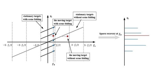
The PRF of each channel is denoted by $f_r$. In a multi-channel system operating in burst mode, the relatively low PRF ensures an unambiguous wide swath. As a result, as long as the target focusing frequency $f_a$ exceeds the limit of PRF, this frequency points will be ambiguous, that is to say, two targets at different positions may focus on the same point in the coarse-focused image domain. This typical phenomenon is called the scene folding in this paper. According to (21), when the azimuth moment ${\eta }_c$ characterizing the position of a stationary target exceeds a specific interval, i.e., $\left[-f_r/2K_a,f_r/2K_a\right]$, the scene will be folded. Therefore, taking the size of the scene into account, (21) is more accurately expressed as

$$f_a+i\cdot f_r=-f_{dc}-K_a{\eta }_c,f_a\in \left[-\frac{f_r}{2},\frac{f_r}{2}\right]andi=-l,-l+1\cdots \cdots ,l-1,l,$$

(22)

where $K=2l+1$ is the number of folding times.

The time-frequency relationship, according to (22), is shown in Figure 3, taking the scene folding five times as an example. The dotted line shows that the stationary targets, e.g., clutter, located at different positions in the scene, will focus on different azimuth frequencies when the system PRF is high enough, and the scene is not superimposed. Furthermore, the solid line represents the time-frequency relationship in the multi-channel ScanSAR system operating in the low PRF. In this way, clutter scattering units located in different positions will focus on the same azimuth frequency point $f_a$ in the coarse-focused image domain at the same time. And there is a distinguishing feature worthy of attention, in which the distribution of these clutter units is equidistant. What is more, owing to the time-frequency relationship of the stationary target is known, it is easy to calculate the azimuth time of clutter units following (22) as

$${\eta }_c=-\frac{f_a}{K_a}+i\cdot \frac{f_r}{K_a},i=-l,-l+1\cdots \cdots ,l-1,l.$$

(23)

Then, we consider the situation with moving targets in the scene, represented with an unbroken red circle in Figure 3. Although the moving target focuses on the same position with several stationary clutter units in the coarse-focused domain, the movement of the target will make it to have an offset along with the Doppler frequency, i.e., $f_{dc}$. Similarly, ambiguity still exists when the frequency exceeds the limitation of a PRF. Which frequency point of the moving target will focus on in the coarse-focused domain is determined by the actual position and velocity of the target together. Unfortunately, we cannot obtain any prior knowledge about such non-cooperative targets as ships. Neither the velocity nor position is known in reality. We, therefore, cannot determine in advance where the moving target will appear. And, in this regard, it is very different from the static clutter unit with a definite time-frequency relationship. What is more, when the energy of the clutter scattering unit is almost equal to or higher than that of the moving target, we need to judge whether there is a moving one. It is precisely the problem solved by the method proposed in this article.

3.2. Scene Folding Times

Before introducing the MTD method, it is necessary to analyze the number of scenes folding times of the echo received by a burst. It tells in Figure 4 that the antenna beam coverage at the start time and end time of a burst illumination time $T_b$. Within this period, the duration corresponding to the complete area illuminated is $T_s+T_b$. Likewise, the length of time corresponding to the effective imaging area is $T_s-T_b$. In the coarse-focused image domain, the size of the scene unfolded is given by

$$\mathsf{\Delta }\eta =\frac{f_r}{K_a}.$$

(24)

Consequently, if we only consider the effective imaging area, the number of scene folding times is calculated by

$$K=\frac{\left(T_s-T_b\right)}{f_r}\cdot K_a.$$

(25)

From (2) and (3), the relationship between $T_b$ and the synthetic aperture time $T_s$ is approximately expressed as

$$T_b=\frac{T_s}{N_B+1}.$$

(26)

And $B_a=T_s\cdot K_a$ is defined as the Doppler bandwidth of the entire scene. $N_{ambi}=B_a/f_r$ represents the number of the main Doppler spectrum ambiguity [33]. Thus, the relationship between the number of folding times $K$ and the Doppler ambiguity $N_{ambi}$ can be expressed as

$$K=N_{ambi}-\frac{1}{N_B+1}{N}_{ambi}.$$

(27)

The multi-channel system requires that the Doppler spectrum ambiguity number $N_{ambi}$ should be less than the number of channels to achieve unambiguous imaging. The number of folding times must be less than the number of channels, as well.

3.3. MTD Based on Sparse Recovery

We assume that there are $I$ moving targets in a particular unit $\left({\tau }_0,f_0\right)$ in the coarse focus domain. Furthermore, the above analysis shows that there are at most $K$ clutter scattering units. According to (19), the signal of the $n$th channel is expressed as:

$$s_n\left({\tau }_0,f_0\right)=s_{n,t}\left({\tau }_0,f_0\right)+s_{n,c}\left({\tau }_0,f_0\right),$$

(28)

where

$$s_{n,t}\left({\tau }_0,f_0\right)={{\displaystyle \sum }}_{l=1}^I\tilde{\sigma }\left(x_l,R_0\right)F\left(f_0,{\mathit{\upsilon }}_{\mathit{t}}^{\left(l\right)}\right)exp\left(-j2\pi K_a{\eta }_c^{\left(l\right)}\left(n-1\right)T_d\right),$$

(29)

$$s_{n,c}\left({\tau }_0,f_0\right)={{\displaystyle \sum }}_{i=1}^K\tilde{\sigma }\left(x_i,R_0\right)F\left(f_0,{\mathit{\upsilon }}_{\mathit{c}}^{\left(\mathit{i}\right)}\right)exp\left(-j2\pi K_a{\eta }_c^{\left(i\right)}\left(n-1\right)T_d\right),$$

(30)

and $\tilde{\sigma }\left(x_{i\left(l\right)},R_0\right)$ can be regarded as a complex constant for a moving target or a clutter unit, where

$$\tilde{\sigma }\left(x_l,R_0\right)={\sigma }^{″}\left(x_l,R_0\right)sinc\left\{B_r\left(\tau -\frac{2R_n\left(f_a\right)}{c}\right)\right\}\cdot W_{f_a}\left(f_a+f_{dc}^{\left(l\right)}+K_a{\eta }_c^{\left(l\right)}\right)\cdot exp\left(-j\cdot \frac{4\pi }{\lambda }{R}_0\right).$$

(31)

Considering in a noisy environment, we express the multi-channel signal (28) in matrix form as

$$\mathit{S}={\mathit{A}}_{\mathit{t}}{\mathit{\sigma }}_{\mathit{t}}+{\mathit{A}}_{\mathit{c}}{\mathit{\sigma }}_{\mathit{c}}+\mathit{n},$$

(32)

where

$$\mathit{S}={\left[S_1\left({\tau }_0,f_0\right),S_2\left({\tau }_0,f_0\right),\cdots \cdots ,S_N\left({\tau }_0,f_0\right)\right]}^T\in {\mathit{R}}^{N\times 1},$$

(33)

$$\mathit{n}={\left[n_1\left({\tau }_0,f_0\right),n_2\left({\tau }_0,f_0\right),\cdots \cdots ,n_N\left({\tau }_0,f_0\right)\right]}^T\in {\mathit{R}}^{N\times 1},$$

(34)

$${\mathit{A}}_{\mathit{t}}=\left[{\mathit{\alpha }}_{\mathbf{1},\mathit{t}},{\mathit{\alpha }}_{\mathbf{2},\mathit{t}},\cdots \cdots ,{\mathit{\alpha }}_{\mathit{I},\mathit{t}}\right]\in {\mathit{R}}^{N\times I},$$

(35)

$${\mathit{A}}_{\mathit{c}}=\left[{\mathit{\alpha }}_{\mathbf{1},\mathit{c}},{\mathit{\alpha }}_{\mathbf{2},\mathit{c}},\cdots \cdots ,{\alpha }_{\mathit{K},\mathit{c}}\right]\in {\mathit{R}}^{N\times K}.$$

(36)

In addition, ${\mathit{\alpha }}_{\mathbf{l},\mathit{t}}$ and ${\mathit{\alpha }}_{\mathit{i},\mathit{c}}$ are the steering vectors of the moving target at ${\eta }_c^{\left(l\right)}$ and the stationary clutter unit at ${\eta }_c^{\left(i\right)}$, respectively. Both of them have the same form of expression written as

$${\mathit{\alpha }}_{\mathit{i}}=\left[\begin{array}{c}\begin{array}{c}1\\ \exp \left(-j2\pi K_a{\eta }_c^{\left(i\right)}{T}_d\right)\end{array}\\ \begin{array}{c}⋮\\ \exp \left(-j2\pi K_a{\eta }_c^{\left(i\right)}\left(N-1\right)T_d\right)\end{array}\end{array}\right],$$

(37)

$${\mathit{\sigma }}_{\mathit{t}}={\left[{\sigma }_{1,t},{\sigma }_{2,t},\cdots \cdots ,{\sigma }_{I,t}\right]}^T\in {\mathit{R}}^{I\times 1},$$

(38)

$${\mathit{\sigma }}_{\mathit{c}}={\left[{\sigma }_{1,c},{\sigma }_{2,c},\cdots \cdots ,{\sigma }_{K,c}\right]}^T\in {\mathit{R}}^{K\times 1},$$

(39)

$${\sigma }_{i,t}=\tilde{\sigma }\left(x_i,R_0\right)F\left(f_0,{\mathit{\upsilon }}_{\mathit{t}}^{\left(i\right)}\right),$$

(40)

$${\sigma }_{i,c}=\tilde{\sigma }\left(x_i,R_0\right)F\left(f_0,{\mathit{\upsilon }}_{\mathit{c}}^{\left(i\right)}\right).$$

(41)

To detect moving targets in the entire effective imaging scene, we divide the effective illumination time $T_s-T_b$ into $P$ grids equidistantly. Then, a signal model based on sparse framework is given by

$$\mathit{S}=\mathit{A}\mathit{\sigma }+\mathit{n},$$

(42)

where

$$\mathit{A}=\left[{\mathit{\alpha }}_{\mathbf{1}},{\mathit{\alpha }}_{\mathbf{2}},\cdots \cdots ,{\mathit{\alpha }}_{\mathit{P}}\right]\in {\mathit{R}}^{N\times P},$$

(43)

$$\mathit{\sigma }=\left[{\sigma }_1,{\sigma }_2,\cdots \cdots ,{\sigma }_P\right]\in {\mathit{R}}^{P\times 1}.$$

(44)

In this case, $\mathit{\sigma }$ is the vector to be recovered, $\mathit{A}$ denotes the over-complete dictionary, which implies all potential locations of targets and clutter units. The number of clutter units is known as $K$, and we believe that moving targets are highly sparse in spatial distribution on the ocean surface. They reflect in the vector $\mathit{\sigma }$, which has a finite number of non-zero values, and all others are zero. Then, ${\eta }_c^{\left(i\right)}$ corresponding to the non-zero value is the location of the moving target or the clutter unit. The sparse vector $\mathit{\sigma }$ is obtained by solving the following problem.

$$\min \parallel \mathit{\sigma }{\parallel }_{l_0}subjectto\parallel \mathit{S}-\mathit{A}\mathit{\sigma }{\parallel }_{{\mathit{l}}_{\mathbf{2}}}<\mathit{\epsilon },$$

(45)

where $\parallel \cdot {\parallel }_{l_i}$ means $l_i$-norm, and $\mathbf{\epsilon }$ is noise power. As we all know, it is a non-deterministic polynomial (NP-hard) problem. Chen, Donoho, and Saunders [39] proposed the method of basis pursuit (BP) to transform the problem of minimizing the $l_0$-norm to minimizing the $l_1$-norm when $\mathit{A}$ meets restricted isometry property (RIP) condition.

$$\min \parallel \mathit{\sigma }{\parallel }_{l_1}subjectto\parallel \mathit{S}-\mathit{A}\mathit{\sigma }{\parallel }_{{\mathit{l}}_{\mathbf{2}}}<\mathit{\epsilon }.$$

(46)

Then, it becomes a convex optimization problem, which can be solved using a linear programming method.

If the number of non-zero values of the signal $\mathit{\sigma }$ is $K_s$, it is called $K_s$-sparse signal. In theory, the sparsity of the signal $K_s$ should be less than or equal to the sum of the number of moving targets $I$ and the scene folding times $K$, i.e.,

$$K_s\le I+K.$$

(47)

There are several cases shown in Figure 5:

Case 1: If there are no moving targets and obvious strong point targets in a uniform scene, such as the sea surface without ships, tropical rainforest, etc., the sparsity $K_s$ is exactly equal to the scene folding times $K$, i.e., $K_s=K$.

Case 2: If there are moving targets in the scene, and its signal-to-clutter ratio (SCR) is relatively high, such as the sea surface with several moving vessels, the sparsity $K_s$ depends on the targets in a specific unit of the coarse-focused image. Given that the high sparseness of moving targets in ocean scenes, there is little possibility of two moving targets focusing on the same point in the coarse focus domain. Consequently, $K_s=1$.

Case 3: If the imaging area is the junction of sea and land, or there is an island in the scene, the moving target may superimpose on the strong clutter in the coarse-focused image domain. It makes us get not only the azimuth time of the moving target but also that of the clutter units from the sparse recovery results. Thus, the number of clutter units is less than the times of scene folding since the spatial distribution of the island is discontinuous. Accordingly, $1<K_s<K$.

Case 4: If there are moving targets in the scene, but the energy of clutter is relatively high, even equivalent to that of moving targets, such as ground moving targets detection from heavy clutter environment, the sparsity $K_s$ is more than the scene folding times $K$, i.e., $K_s>K$.

In this manuscript, we are concerned about the detection of moving ships in ocean scenes with or without the island, that is, case 2 and case 3. The proposed method can indicate moving targets more effectively and accurately, benefiting from the advantages of sparse spatial distribution and high signal energy of such ocean scenes.

Next, we will pay attention to how to distinguish moving targets and stationary ones from sparse recovery results. Assuming that $f_0$ is the selected azimuth frequency point containing the moving target possibly, the fixed time-frequency relationship of stationary clutter as (23) makes it easy to calculate their azimuth times. For convenience, we express the calculated results again as

$${\eta }_{ci,cal}=-\frac{f_a}{K_a}+i\cdot \frac{f_r}{K_a},i=-l,-l+1\cdots \cdots ,l-1,l.$$

(48)

We can get $K$ values through calculation, and ${\eta }_{ci,cal}$ indicates the correct azimuth position of the stationary target. Meanwhile, we get $K_s$ estimated results from sparse recovery. Because the real position of the moving target focused on the selected azimuth frequency point $f_0$ is different from the calculated position of the stationary targets, we can identify which is the moving target by comparing each estimated result with the calculated results. In practice, the calculated value and the estimated one cannot be consistent absolutely. This acceptable error is closely related to the expected velocity and positioning accuracy. And the next part will solve this problem.

3.4. Radial Velocity Estimation and Positioning

Supposing that a moving target locates at $f_0,$ for convenience of description, the estimation results of the sparse recovery can be written as

$${\eta }_{ci,est}={\eta }_{c0,est}+i\cdot \frac{f_r}{K_a},{\eta }_{c0,est}\in \left[-\frac{f_r}{2K_a},\frac{f_r}{2K_a}\right]\mathrm{and} i=-l,-l+1\cdots \cdots ,l-1,l,$$

(49)

where ${\eta }_{c0,est}$ is a baseband azimuth time free from ambiguous. Of course, the azimuth time when the target appears is still represented by ${\eta }_{ci,est}$. From (6), the azimuth coordinates of the moving target are calculated by

$$x_0={\eta }_{ci,est}\cdot v_s.$$

(50)

We can also obtain its radial velocity information according to (12), (22), and (49).

$$v_r=\frac{\lambda }{2}\left(-f_a-K_a{\eta }_{c0,est}\right),f_a\in \left[-\frac{f_r}{2},\frac{f_r}{2}\right].$$

(51)

Then, an inequality is derived from (51) as

$$-\frac{f_r}{2}\le -\frac{2v_r}{\lambda }-K_a{\eta }_{c0,est}\le \frac{f_r}{2},m\left({\eta }_{c0,est}\right)-v_{max}\le v_r\le m\left({\eta }_{c0,est}\right)+v_{max},$$

(52)

where

$$v_{max}=\frac{f_r\lambda }{4},$$

(53)

$$m\left({\eta }_{c_0}\right)=-\frac{K_a{\eta }_{c0,est}\lambda }{2}.$$

(54)

Notably, the range of detectable velocity is related to the azimuth time of the target, implied in Figure 6a. The rectangular is the area where the estimated velocity value is located. The light shadow area between the two red lines is the correct velocity estimation range, while the estimated results of two dark triangle shadow areas will be ambiguous. The Doppler frequency shift caused by radial velocity cannot exceed PRF of the system. Accordingly, the equation for calculating the radial velocity given by (51) equation requires the moving target to fall in the region without ambiguity, i.e., the light shadow area. Unfortunately, if the position of the target just falls in the ambiguous velocity area, additional modification of the estimated result is needed. Taking the negative azimuth chirp rate $\left(K_a<0\right)$ as an example, the correction process is expressed as

$$v_r=\{\begin{array}{cc}{v}_r+v_{max}& {\eta }_c>0\\ v_r& {\eta }_c=0\\ v_r-v_{max}& {\eta }_c<0\end{array}.$$

(55)

The whole modification process is illustrated in Figure 6b, which is equivalent to shifting the position of two dark triangle areas along the frequency axis. In that case, the range of estimated radial velocity is identical no matter where it is, i.e.,

$$\left|v_r\right|\le v_{max}$$

(56)

Consequently, the maximum detectable velocity (MDV) is $v_{max}$, which is depend on PRF and wavelength only.

Finally, let us discuss the acceptable errors mentioned in the previous section. If the error of the sparse recovery results is $\pm {\eta }_{c,error}$, the error of the estimated target position $x_{0,error}$ is calculated as $\pm \left|{\eta }_{c,error}\cdot v_s\right|$, and the error of the estimated velocity $v_{r,error}$ is calculated as $\pm \left|{\eta }_{c,error}\cdot K_a\right|\cdot \mathsf{\lambda }/2$. In the practical application, the desired velocity or positioning accuracy determines the acceptable error. Finally, the detailed processing flow chart of the proposed MTD method is summarized in Figure 7.

4. Simulation Results

The effectiveness of the proposed MTD approach is verified in this section using a simulation system. The relevant system parameters are listed in

Table 1. Parameters of the simulation system.

Symbol	Parameter	Value
$\lambda$	Wavelength	0.055517 m
$B_r$	Signal bandwidth	120 MHz
$F_s$	Sampling rate	150 MHz
$T_r$	Pulse width	30 $\mathsf{\mu }\mathrm{s}$
$N$	Channel number	6
$d$	Baseline	1.4 m
$v_s$	Platform velocity	7508 m/s
$R_0$	Reference slant range	800 Km
$f_r$	PRF	1340.7 Hz
$T_s$	Synthetic aperture time	2.11 s
$T_b$	Dwell time of a burst	0.52 s
$B_a$	Doppler bandwidth	5362.9 Hz
$K$	Scene folding times	3

.

The first thing we will talk about is what is an acceptable error in the simulation system in which parameters are listed in Table 1. If we expect to control the radial measurement error within $\pm 0.5 \mathrm{m}/\mathrm{s}$ and the positioning error within $\pm 50 \mathrm{m}/\mathrm{s}$, then the result error of the sparse recovery must be controlled within 0.007 s. Hence, the target is considered as a moving one when the difference between the calculated value ${\eta }_{ci,cal}$ and the actual result of sparse recovery ${\eta }_{ci,est}$ exceeds 0.007 s. And from (53), the MDV is $18.61 \mathrm{m}/\mathrm{s}$.

4.1. Different Scenes

To verify the detection ability of the proposed method in different situations, we set up three typical scenarios. Scene 1 is static clutter without any moving targets, shown in Figure 8a. It should be noted that the multi-channel echoes of the sea clutter background or island in the following simulation scenarios are the result of the convolution of a part of backscattering coefficients on GaoFen-3 (GF-3) image and the multi-channel echo of the stationary point target. In Scene 2, there is a moving target on the clutter background. However, from Figure 8b, there are two false targets (also called ghost targets) on both sides of the real one. In the multi-channel system, the unambiguous imaging algorithm is developed for static scenes. But, for moving targets, azimuth Doppler ambiguity still exists after imaging [34]. The moving target detection method operating in the coarse-focused domain proposed in this paper avoids the adverse effect of Doppler ambiguity. In the actual SAR data processing process, we often encounter the situation that there are islands in the ocean scenes. In addition, the energy of the island is stronger than that of the clutter and is the nearest equivalent to the moving target energy, which is the reason why we simulate Scene 3, just as Figure 8c. In this scenario, there is a moving target and a stationary target to simulate a strong scattering point on the island. For clarity, the specific design scheme of each scene is listed in

Table 2. Design schemes of the three scenes.

Scene Number	Design Scheme
$1$	Stationary clutter
$2$	Stationary clutter A moving target: ${\eta }_c=-0.2238 \mathrm{s}, v_r=3.5 \mathrm{m}/\mathrm{s}$
$3$	Stationary island A moving target: ${\eta }_c=-0.0746 \mathrm{s}, v_r=3.5 \mathrm{m}/\mathrm{s}$ Static target 1: ${\eta }_{c1}=0.5033 \mathrm{s}$

. Parameter ${\eta }_c$ in the table is the azimuth time related to the target position, as shown in (6).

The coarse-focused images of the three scenes are shown in Figure 8d–f, respectively. Particular attention should be paid to the result of scene 3. Although the island and the moving target do not overlap in spatial distribution, they superimpose on each other in the coarse-focused imaging. It is the phenomenon of scene folding. Next, we separately detect moving targets in the three scenes employing the sparse recovery.

Since there is no moving target in scene 1, we arbitrarily choose an azimuth frequency point $f_a=0 \mathrm{Hz}$ to analyze the sparse recovery results. From Figure 8g, the result tells that there are three targets here, located at ${\eta }_{c-1,est}=-0.527 \mathrm{s}$, ${\eta }_{c0,est}=-0.002 \mathrm{s}$, and ${\eta }_{c1,est}=0.527 \mathrm{s}$. How can we know which of these three targets is a stationary one and which is a moving one? Because the selected azimuth frequency point $f_a$ is known, we can easily find the positions of the stationary targets by (48). Therefore, when $f_a=0 \mathrm{Hz}$, the calculated positions of the stationary targets should be ${\eta }_{c-1,cal}=-0.528 \mathrm{s},$ ${\eta }_{c0,cal}=0 \mathrm{s}$, and ${\eta }_{c1,cal}=0.528 \mathrm{s}$, which is very close to the experimental results. The maximum error is $0.002 \mathrm{s}$, which is less than the preset acceptable error $0.007 \mathrm{s}$. As a result, none of the three targets we see is a moving one. It just verified Case 1 mentioned in the previous section: the sparsity $K_s$ is exactly equal to the scene folding times $K$, that is, $K_s=3$. For scene 2, a strong point appears at $f_a=441.22 \mathrm{Hz}$. The sparse recovery results for this point are shown in Figure 8h. Because SCR is high enough, we only see one target at ${\eta }_{c0,est}=-0.223 \mathrm{s}$. According to (48), if it is a stationary target, its possible position is ${\eta }_{c-1,cal}=-0.702 \mathrm{s}$, ${\eta }_{c0,cal}=-0.174 \mathrm{s}$, or ${\eta }_{c1,cal}=0.354 \mathrm{s}$. The error between the estimated value and the calculated value is $0.049 \mathrm{s}$, which is over the acceptable error $0.007 \mathrm{s}$. Obviously, the strong point target seen in the experimental results is a moving target. The radial velocity of the target is calculated as $3.47 \mathrm{m}/\mathrm{s}$ from (51), which is almost the same as the ideal value $3.5 \mathrm{m}/\mathrm{s}$ set in the experiment. Scene 2 is also a typical example of Case 2 mentioned in the previous section, where $K_s=1$.

The strong point target in scene 3 focuses on the azimuth frequency point $f_a=58.70 \mathrm{Hz}$. From the result of the sparse recovery in Figure 8i, there are two strong targets superimposed here. Similarly, the positions where the static units of this azimuth frequency point should appear are calculated by (48) as: ${\eta }_{c-1,cal}=-0.552 \mathrm{s}$, ${\eta }_{c0,cal}= -0.023 \mathrm{s}$, and ${\eta }_{c1,cal}=0.505 \mathrm{s}$. Compared with the experimental results, one of two targets in which the estimated result is ${\eta }_{c1,est}=0.502 \mathrm{s}$ is very close to the calculated theoretical value ${\eta }_{c1,cal}=0.505 \mathrm{s}$ within an acceptable error, so we consider this one to be stationary. However, the target at ${\eta }_{c0,est}=-0.072 \mathrm{s}$ is a moving target. Its velocity is calculated to be $3.44 \mathrm{m}/\mathrm{s}$, and the error with the ideal value is $0.06 \mathrm{m}/\mathrm{s}$. And the positioning error is $19.5 \mathrm{m}$.

4.2. MTD Effect Demonstration

In addition, the proposed method based on sparse recovery can achieve the functions of moving target detection, radial velocity information acquisition, and target positioning at the same time.

Another simulation experiment, arranged nine-point targets, including four moving targets and five stationary ones, is carried out to demonstrate the effect of the proposed MTD method. The details of the experiment are recorded in

Table 3. Nine-point scene experiment results.

Point	$\mathbf{Select} {\mathit{f}}_{\mathit{a}}$	${\mathit{\eta }}_{\mathit{c}0,\mathit{c}\mathit{a}\mathit{l}} \mathbf{Calculated} \mathbf{by} \left(48\right)$	${\mathit{\eta }}_{\mathit{c}0,\mathit{e}\mathit{s}\mathit{t}} \mathbf{Estimated}$	$\left|{\mathit{\eta }}_{\mathit{c}0,\mathit{e}\mathit{s}\mathit{t}}-{\mathit{\eta }}_{\mathit{c}0,\mathit{c}\mathit{a}\mathit{l}}\right|$	${\mathit{v}}_{\mathit{r}} \mathbf{Estimated} \mathbf{by} \left(51\right)$	Whether It Is a Moving Target?	${\mathit{x}}_0 \mathbf{Location} \mathbf{Estimation} \mathbf{by} \left(50\right)$
1	−568.09 Hz	0.224 s	0.225 s	0.001 s	−0.0846 m/s	No
2	−388.20 Hz	0.153 s	0.224 s	0.071 s	−5.0078 m/s	Yes	1681.792 m
3	−568.09 Hz	0.224 s	0.224 s	0 s	−0.0142 m/s	No
4	−287.83 Hz	0.113 s	0.001 s	0.112 s	7.9194 m/s	Yes	7.508 m
5	0 Hz	0 s	0	0 s	0 m/s	No
6	215.88 Hz	−0.085 s	−0.001 s	0.084 s	−5.9219 m/s	Yes	−7.508 m
7	568.09 Hz	−0.223 s	−0.224 s	0.001 s	0.0142 m/s	No
8	208.30 Hz	−0.082 s	−0.225 s	0.143 s	10.0719 m/s	Yes	−1689.300 m
9	568.09 Hz	−0.224 s	−0.224 s	0 s	0.0142 m/s	No

. And the effect of moving target detection is shown in Figure 9b. The moving target will offset a certain distance along the azimuth direction in SAR image, which is proportional to the radial velocity. The position of the yellow circle is that of the moving target in the SAR image, and the place marked with “×” is the real position of the target obtained by MTD proposed method based on sparse recovery. In the meantime, the experimental results verified the effectiveness of the proposed method in detection, velocity estimation, and relocation.

4.3. Unambiguous Imaging of Moving Targets

From Figure 9b, the MTD method proposed in this manuscript indicates which one is the moving target, as well as estimates the radial velocity and the true azimuth position of the target successfully. But, in some applications, we hope to get an unambiguous imaging result of moving targets free from the false targets and expect the moving targets to focus on their correct positions instead of just marking them. An unambiguous imaging scheme of moving targets for maritime scenarios is proposed in Reference [34]. One of the important steps is to compensate for the phase term introduced by the radial velocity. Fortunately, the MTD method proposed in this manuscript can also measure the radial velocity of the moving target, which helps suppress the azimuth ambiguity. To show the imaging results of moving targets more specifically, we only focus on the four moving targets in Figure 9. The imaging results without any motion phase compensation are shown in Figure 10a. The radial velocities of four moving targets are recorded in Table 3, which are −5.0078 m/s, 7.9194 m/s, −5.9219 m/s, and 10.0719 m/s, respectively. The imaging result after compensating the phase term caused by velocity is shown in Figure 10b. After the motion compensation, the false target in the image is greatly suppressed, just as illustrated in Figure 10c,d, and the position of the moving target is corrected. This work reduces the difficulty of image interpretation next.

5. Performance Analysis

This section analyzes several performances of the proposed method theoretically and experimentally. Firstly, we interpret that the over-complete dictionary matrix in this paper is equivalent to the sensing matrix in the compressed sensing model, and the correlation between atoms of the matrix is utilized to measure the performance of sparse recovery. Then, Monte Carlo experiments are carried out to verify the performance of the proposed method under different SCR conditions.

5.1. Rationality Analysis

Compressed sensing (CS) is an effective theoretical basis for recovering sparse signals. At first, we will explain the rationality of our signal model in (42) applied to CS theory [40], which addresses the following problem:

$$\mathit{y}=\mathit{\Phi }\mathit{x}=\mathit{\Phi }\mathit{\Psi }\mathit{d}=\mathit{\Theta }\mathit{d},$$

(57)

where the signal $\mathit{x}$ is assumed to be sparse or compressible in some sparse basis $\mathit{\Psi }\in R^{P\times P}$, the signal $\mathit{d}$ is a $K_s$-sparse signal. Furthermore, $\mathit{\Phi }$ is the measurement matrix of the size $N\times P$ with $N<P$. The main goal of CS is to recover the $K_s$-sparse signal $\mathit{d}$ of length $P$ from measurements signal $\mathit{y}$ of length $N$.

From (42), the received multi-channel signal $\mathit{S}$ is modeled as a superposition of $K_s$ target signals. The high SCR of the ocean scene makes $K_s$ equal to 1 in most cases except for the particular example of the target and an island superposition in the coarse-focused image domain. There is a one-to-one correspondence between the location of the target $x_0$ and the azimuth moment ${\eta }_c$ when the target appears. Therefore, sparsity in spatial distribution is equivalent to that in azimuth time. Correspondingly, we divide the effective illumination time of a burst into $P$ grids. If we want to get the information of each target in the $P$ grids, we must have $P$ measurements. Hence, the basis matrix is given by

$$\widetilde{\mathit{A} }=\left[\widetilde{{\mathit{\alpha }}_{\mathbf{1}}},\widetilde{{\mathit{\alpha }}_{\mathbf{2}}},\cdots \cdots ,\widetilde{{\mathit{\alpha }}_{\mathit{p}}}\right]\in {\mathit{R}}^{P\times P} ,$$

(58)

where

$$\widetilde{{\mathit{\alpha }}_{\mathit{i}}}=\left[\begin{array}{c}\begin{array}{c}1\\ exp\left(-j2\pi K_a{\eta }_c^{\left(i\right)}{T}_d\right)\end{array}\\ \begin{array}{c}⋮\\ exp\left(-j2\pi K_a{\eta }_c^{\left(i\right)}\left(P-1\right)T_d\right)\end{array}\end{array}\right] .$$

(59)

Whereas the signal is compressible, i.e., $K_s\ll P$, we only need $N$ measurements to get an estimation of the signal. In the same way, the measurement matrix is defined as $\mathit{\Phi }={\mathit{I}}_{\mathit{N}\times \mathit{P}}$, that is, the first $N$ rows of the $P$-dimensional identity matrix. In this case, the signal model in (42) can also be expressed as the following equation corresponding to the CS model.

$$\mathit{S}=\mathit{\Phi }\tilde{\mathit{A}}\mathit{\sigma }=\mathit{A}\mathit{\sigma } .$$

(60)

Consequently, the over-complete dictionary $\mathit{A}$ in (43) is the sensing matrix $\mathit{\Theta }$ of CS model. Note, this problem formulation imposes that the actual moving target signal is many fewer than the potential ones. Although RIP theory is a sufficient condition to test whether a matrix can reconstruct a signal, it is complicated to judge whether a matrix satisfies the requirement. Another criterion is expressed in Reference [41]: When the number of measured values $N$, the signal dimension $P$, and the sparsity $K_s$ of the signal satisfy $N\ge K_{s}logP$, it means that the low-dimensional received echo $\mathit{S}$ already contains enough information to reconstruct the signal $\mathit{\sigma }$.

Subsequently, what we are interested in is the factor that affects signal reconstruction. In CS theory, the correlation between columns in the sensing matrix is also an index to evaluate the performance of reconstruction [42]. The smaller the correlation, the better the reconstruction performance. Let

$$\mu \left(A\right)=\max \frac{\left|{\alpha }_i^H{\alpha }_j\right|}{\parallel {\alpha }_i{\parallel }_{l2}\cdot \parallel {\alpha }_j{\parallel }_{l2}},i,j=1,2,\cdots \cdots ,Pi\ne j.$$

(61)

By substituting (37) into (61), the correlation coefficient is written as

$$\mu \left(A\right)=\max \frac{\left|sin\left(N\pi K_a{T}_d\left({\eta }_c^{\left(i\right)}-{\eta }_c^{\left(j\right)}\right)\right)\right|}{N sin\left(\pi K_a{T}_d\left({\eta }_c^{\left(i\right)}-{\eta }_c^{\left(j\right)}\right)\right)} =\max \frac{\left|sin\left(N\pi \frac{d{v}_s}{\lambda R_0}\left({\eta }_c^{\left(i\right)}-{\eta }_c^{\left(j\right)}\right)\right)\right|}{N sin\left(\pi \frac{d{v}_s}{\lambda R_0}\left({\eta }_c^{\left(i\right)}-{\eta }_c^{\left(j\right)}\right)\right)}.$$

(62)

Without loss of generality, we defined ${\eta }_c^{\left(i\right)}-{\eta }_c^{\left(j\right)}$ as the interval of the grid $\mathsf{\Delta }{\eta }_c$. The formula implies that the correlation coefficient is related to the interval of the grid and the antenna length $L$. Even though the increase of grid interval is beneficial to improve the performance of sparse signal recovery from Figure 11, it should be reasonably selected to realize the super-resolution estimation of the position of the moving target. Figure 11a shows that with the identical antenna baseline $d$, the more channels are, the less correlation of the sensing matrix is. Similarly, with the same number of channels, the performance will be better with the increase of antenna baseline, which is demonstrated in Figure 11b. In comparison, under the assumption of fixed antenna length $L$, the combination of different baseline length and channel number shows the same performance, implied in Figure 11c. In brief, for the sake of ensuring the super-resolution estimation ability, we may not be able to improve the performance of sparse signal recovery by merely increasing the time interval of the grid. However, the increase in antenna length will allow multiple targets folded in a unit in the coarse-focused imaging domain, such as ground moving targets detection.

Moreover, in this manuscript, the number of pulses (also called snapshots) used to recover sparse signals is one, i.e., single measurement vector (SMV). In future work, the application of multiple measurement vector (MMV) will improve the accuracy of the reconstructed signal undoubtedly.

5.2. Influence of SCR in Coarse-Focused Imaging Domain

There is no doubt that the power of clutter background will, to some extent, affect the performance of moving target detection. In the image, different SCR reflect various clutter environments. Besides, both external and internal factors of the MTD method works in the coarse focused domain, the influence of different signal-to-noise ratio (SNR) and SCR in this domain will be elaborated experimentally in this section.

Since the SNR of the echo signal will improve greatly after range compression and azimuth dechirp, the noise in the coarse focus domain will not be too strong. We take point target as an example to illustrate it. In the worst case, the noise and the signal have the same energy, i.e., SNR = 0 dB, in the echo domain. After the matched filtering in range direction, the SNR has increased by 20 dB. And after dechirp operation in the azimuth direction, the SNR has increased by 20 dB again. It qualitatively shows that SNR in the coarse focus domain is significantly higher than that in the echo domain.

Then, 500 Monte Carlo tests were carried out to explore the performance of the proposed method under different SCR and SNR conditions, i.e.,$N_{MC}=500$, shown in Figure 12. The SCR is set from 10 dB to 40 dB, while SNR is from 30 dB to 40 dB. The root-mean-square error (RMSE) is used to evaluate the accuracy of the estimation. Suppose that the result of the sparse recovery of a test is ${\widehat{\eta }}_{c,est}$ and the real value is ${\eta }_c$. The error is calculated by

$${\eta }_{rmse}=\sqrt{\frac{1}{N_{MC}}{\displaystyle \sum }_{i=1}^{N_{MC}}{\left({\widehat{\eta }}_{c,est}^{\left(i\right)}-{\eta }_c\right)}^2}.$$

(63)

We consider this test is successful if the difference between the estimated result ${\widehat{\eta }}_{c,est}$ and the real value ${\eta }_c$ of a single test is less than 0.007 s. Assuming that the number of successful trials in $N_{MC}$ trials is $N_{suc}$, then the success rate $R_{suc}$ is written as

$$R_{suc}=\frac{N_{suc}}{N_{MC}}\times 100\%.$$

(64)

From Figure 12a, the information we get is that the estimation error is relatively small when SCR in the coarse-focused domain is over 20 dB. Similarly, when SCR is over 20 $\mathrm{dB}$, the success rate is relatively high from Figure 12b.

GF-3 is the first Chinese multi-channel SAR sensor with dual receive channels [43] named ultra-fine stripmap (UFS) mode. In order to investigate the approximate SCR of the marine moving targets in the actual data, we selected 18 images of the Huanghai Sea (starting at E123.9, 34.2N, and ending at E122.9, N29.4) collected by GF-3 SAR sensor on 18 May 2019. And the SCR values of 57 ships in the coarse-focused domain are calculated and displayed in Figure 13. Generally speaking, if the sea surface condition is complex, such as affected by a strong wind field, the SCR is relatively low. On the other hand, the SCR of the target on the calm sea surface is relatively high. However, from the statistical results of the actual data, the SCR is almost no less than 20 $\mathrm{dB}$. Therefore, to some extent, the proposed MTD method is suitable for most kinds of the sophisticated or calm sea surface. We do not give too much consideration to the influence of some extreme atmospheric conditions. Because it is very difficult to produce a high-quality image under such conditions, moving target detection and ambiguity suppression will become meaningless.

What is more, moving target detection in the scene with lower SCR corresponds to ground moving target detection (GMTI). Following the previous conclusion, due to the limited number of observations, the accuracy of sparse recovery reduces.

6. Conclusions

This paper suggests a marine MTD method based on the sparse recovery idea. The advantages of this method are summarized as follows: (1) Moving targets are detected in the coarse-focused domain, which avoids the influence of false targets after imaging. (2) It is more efficient compared with the traditional STAP method by avoiding the velocity iteration. (3) The proposed approach integrates the detection, radial velocity measurement, and repositioning, as well as comprehensively grasps the motion information of the ships on the vast sea surface. (4) It takes full advantage of the characteristics of high SCR and the highly sparse distribution of moving targets in the ocean scene. (5) The radial velocity measured by the proposed MTD method helps suppress the azimuth ambiguity. Statistics suggest that the SCR of moving target in the coarse-focused domain is usually not less than 20 dB in various ocean scenes. The experimental results tell that the proposed method has excellent performance when the SCR is higher than 20 dB. However, this method also has some limitations. For the scene with low SCR or continuous distribution of strong scattering area, e.g., scenes of land, limited by the number of observations, it may not achieve the effect of moving target detection. In the future, this method is expected to realize engineering and automatic operation. And the algorithm has great social value in many application fields, such as ship search and rescue and route prediction.

References

- Tomiyasu, K. Tutorial review of synthetic-aperture radar (SAR) with applications to imaging of the ocean surface. Proc. IEEE 1978, 66, 563–583. [Google Scholar] [CrossRef]
- Tomiyasu, K. Image processing of synthetic aperture radar range ambiguous signals. IEEE Trans. Geosci. Remote Sens. 1994, 32, 1114–1117. [Google Scholar] [CrossRef]
- Freeman, A.; Johnson, W.T.K.; Huneycutt, B.; Jordan, R.; Hensley, S.; Siqueira, P.; Curlander, J. The “Myth” of the minimum SAR antenna area constraint. IEEE Trans. Geosci. Remote Sens. 2000, 38, 320–324. [Google Scholar] [CrossRef] [Green Version]
- Currie, A.; Brown, M.A. Wide-swath SAR. IEE Proc. F Radar Signal Process. 1992, 139, 125–135. [Google Scholar] [CrossRef]
- Gebert, N.; Krieger, G.; Moreira, A. Digital Beamforming on Receive: Techniques and Optimization Strategies for High-Resolution Wide-Swath SAR Imaging. IEEE Trans. Aerosp. Electron. Syst. 2009, 45, 564–592. [Google Scholar] [CrossRef] [Green Version]
- Yang, T.; Li, Z.; Suo, Z.; Bao, Z. Performance Analysis for Multichannel HRWS SAR Systems Based on STAP Approach. IEEE Trans. Geosci. Remote Sens. 2013, 10, 1409–1413. [Google Scholar] [CrossRef]
- Krieger, G.; Gebert, N.; Moreira, A. Unambiguous SAR signal reconstruction from nonuniform displaced phase center sampling. IEEE. Geosci. Remote Sens. Lett. 2004, 1, 260–264. [Google Scholar] [CrossRef] [Green Version]
- Krieger, G.; Gebert, N.; Moreira, A. Multichannel Azimuth Processing in ScanSAR and TOPS Mode Operation. IEEE Trans. Geosci. Remote Sens. 2010, 48, 2994–3008. [Google Scholar]
- Yang, W.; Li, C.; Wang, P.; Chen, J. Performance analysis and data processing of space-borne multi-channel ScanSAR Mode for high-resolution wide-swath. In Proceedings of the IET International Radar Conference 2009, Guilin, China, 20–22 April 2019. [Google Scholar]
- Krieger, G.; Younis, M.; Gebert, N.; Huber, S.; Bordoni, F.; Patyuchenko, A.; Moreira, A. Advanced concepts for high-resolution wide-swath SAR imaging. In Proceedings of the 8th European Conference on Synthetic Aperture Radar, Aachen, Germany, 7–10 June 2010; pp. 524–527. [Google Scholar]
- Gebert, N.; Krieger, G.; Younis, M.; Bordoni, F.; Moreira, A. Ultra wide swath imaging with multi-channel ScanSAR. In Proceedings of the IGARSS 2008—2008 IEEE International Geoscience and Remote Sensing Symposium, Boston, MA, USA, 7–11 July 2008; pp. 21–24. [Google Scholar]
- Rousseau, L.; Gierull, C.; Chouinard, J. First Results from an Experimental ScanSAR-GMTI Mode on RADARSAT-2. IEEE J. Sel. Top. Appl. Earth Obs. Remote Sens. 2015, 8, 5068–5080. [Google Scholar] [CrossRef]
- Gierull, C.H.; Sikaneta, I.C. Raw data based two-aperture SAR ground moving target indication. In Proceedings of the IEEE International Geoscience and Remote Sensing Symposium, Toulouse, France, 21–25 July 2003; pp. 1032–1034. [Google Scholar]
- Lightstone, L.; Faubert, D.; Rempel, G. Multiple phase centre DPCA for airborne radar. In Proceedings of the IEEE National Radar Conference, Los Angeles, CA, USA, 12–13 March 1991; pp. 36–40. [Google Scholar]
- Zebker, H.A.; Goldstein, R.M. Topographic mapping from interferometric synthetic aperture radar observations. J. Geophys. Res. Solid Earth 1986, 91, 4993–4999. [Google Scholar] [CrossRef]
- Breit, H.; Eineder, M.; Holzner, J.; Runge, H.; Bamler, R. Traffic monitoring using SRTM along-track interferometry. In Proceedings of the IEEE International Geoscience and Remote Sensing Symposium, Toulouse, France, 21–25 July 2003; pp. 1187–1189. [Google Scholar]
- Ender, J.H.G. Space-time processing for multichannel synthetic aperture radar. Electron. Commun. Eng. J. 1999, 11, 29–38. [Google Scholar] [CrossRef]
- Ward, J. Space-time adaptive processing for airborne radar. In Proceedings of the IEE Colloquium on Space-Time Adaptive Processing, London, UK, 6 April 1998; pp. 2/1–2/6. [Google Scholar]
- Friedlander, B.; Porat, B. VSAR: A high resolution radar system for detection of moving targets. IEE Proc. Radar Sonar Navigat. 1997, 144, 205–218. [Google Scholar] [CrossRef]
- Jansen, R.W.; Raj, R.G.; Rosenberg, L.; Sletten, M.A. Practical Multichannel SAR Imaging in the Maritime Environment. IEEE Trans. Geosci. Remote Sens. 2018, 56, 4025–4036. [Google Scholar] [CrossRef]
- Guo, X.; Gao, Y.; Liu, X. Moving target detection in HRWS mode. In Proceedings of the IEEE International Geoscience and Remote Sensing Symposium, Fort Worth, TX, USA, 23–28 July 2017; pp. 1169–1172. [Google Scholar]
- Hou, L.; Song, H.; Zheng, M.; Zhang, L.; Qi, L. Clutter suppression for multichannel synthetic aperture radar ground moving target indication system with the capability of high-resolution wide-swath imaging. J. Appl. Remote Sens. 2015, 9, 095054. [Google Scholar] [CrossRef]
- Zhang, S.; Xing, M.; Xia, X.; Guo, R.; Liu, Y.; Bao, Z. A Novel Moving Target Imaging Algorithm for HRWS SAR Based on Local Maximum-Likelihood Minimum Entropy. IEEE Trans. Geosci. Remote Sens. 2014, 52, 5333–5348. [Google Scholar] [CrossRef]
- Wang, L.; Wang, D.; Li, J.; Xu, J.; Xie, C.; Wang, L. Ground Moving Target Detection and Imaging Using a Virtual Multichannel Scheme in HRWS Mode. IEEE Trans. Geosci. Remote Sens. 2016, 54, 5028–5043. [Google Scholar] [CrossRef]
- Baumgartner, S.V.; Krieger, G. Simultaneous High-Resolution Wide-Swath SAR Imaging and Ground Moving Target Indication: Processing Approaches and System Concepts. IEEE J. Sel. Top. Appl. Earth Obs. Remote Sens. 2015, 8, 5015–5029. [Google Scholar] [CrossRef]
- Shu, Y.; Liao, G.; Yang, Z. Design Considerations of PRF for Optimizing GMTI Performance in Azimuth Multichannel SAR Systems with HRWS Imaging Capability. IEEE Trans. Geosci. Remote Sens. 2014, 52, 2048–2063. [Google Scholar]
- Yang, T.; Li, Z.; Suo, Z.; Bao, Z. Ground moving target indication for high-resolution wide-swath synthetic aperture radar systems. IET Radar Sonar Navig. 2014, 8, 227–232. [Google Scholar] [CrossRef]
- Zhang, S.; Xing, M.; Xia, X.; Guo, R.; Liu, Y.; Bao, Z. Robust Clutter Suppression and Moving Target Imaging Approach for Multichannel in Azimuth High-Resolution and Wide-Swath Synthetic Aperture Radar. IEEE Trans. Geosci. Remote Sens. 2015, 53, 687–709. [Google Scholar] [CrossRef]
- Zheng, H.; Wang, J.; Liu, X. Ground Moving Target Indication for High-Resolution Wide-Swath Synthetic Aperture Radar Systems. IEEE. Geosci. Remote Sens. Lett. 2017, 14, 749–753. [Google Scholar] [CrossRef]
- Kim, J.; Younis, M.; Prats-Iraola, P.; Gabele, M.; Krieger, G. First Spaceborne Demonstration of Digital Beamforming for Azimuth Ambiguity Suppression. IEEE Trans. Geosci. Remote Sens. 2013, 51, 579–590. [Google Scholar] [CrossRef] [Green Version]
- Yang, T.; Li, Z.; Liu, Y.; Bao, Z. Channel Error Estimation Methods for Multichannel SAR Systems in Azimuth. IEEE. Geosci. Remote Sens. Lett. 2013, 10, 548–552. [Google Scholar] [CrossRef]
- Shang, M.; Qiu, X.; Han, B.; Ding, C.; Hu, Y. Channel Imbalances and Along-Track Baseline Estimation for the GF-3 Azimuth Multichannel Mode. Remote Sens. 2019, 11, 1297. [Google Scholar] [CrossRef] [Green Version]
- Jin, T.; Qiu, X.; Hu, D.; Ding, C. An ML-Based Radial Velocity Estimation Algorithm for Moving Targets in Spaceborne High-Resolution and Wide-Swath SAR Systems. Remote Sens. 2017, 9, 404. [Google Scholar] [CrossRef] [Green Version]
- Yang, J.; Qiu, X.; Zhong, L.; Shang, M.; Ding, C. A Simultaneous Imaging Scheme of Stationary Clutter and Moving Targets for Maritime Scenarios with the First Chinese Dual-Channel Spaceborne SAR Sensor. Remote Sens. 2019, 11, 2275. [Google Scholar] [CrossRef] [Green Version]
- Calloway, T.M.; Donohoe, G.W. Subaperture autofocus for synthetic aperture radar. IEEE Trans. Aerosp. Electron. Syst. 1994, 30, 617–621. [Google Scholar] [CrossRef]
- Wahl, D.E.; Eichel, P.H.; Ghiglia, D.C.; Jakowatz, C.V. Phase gradient autofocus-a robust tool for high resolution SAR phase correction. IEEE Trans. Aerosp. Electron. Syst. 1994, 30, 827–835. [Google Scholar] [CrossRef] [Green Version]
- Li, S.; Zhang, S.; Mei, S.; Liu, Q.; Wan, S. A Moving Target Imaging Algorithm Based on Compressive Sensing for Multi-channel in Azimuth HRWS SAR System. In Proceedings of the 6th Asia-Pacific Conference on Synthetic Aperture Radar (APSAR), Xiamen, China, 26–29 November 2019. [Google Scholar]
- Middleton, R.J.C. Dechirp-on-Receive Linearly Frequency Modulated Radar as a Matched-Filter Detector. IEEE Trans. Aerosp. Electron. Syst. 2012, 48, 2716–2718. [Google Scholar] [CrossRef]
- Chen, S.S.; Donoho, D.L.; Saunders, M.A. Atomic Decomposition by Basis Pursuit. SIAM Rev. 2001, 43, 129–159. [Google Scholar] [CrossRef] [Green Version]
- Donoho, D.L. Compressed sensing. IEEE Trans. Inf. Theory 2006, 52, 1289–1306. [Google Scholar] [CrossRef]
- Schmidt, R. Multiple emitter location and signal parameter estimation. IEEE Trans. Antennas Propag. 1986, 34, 276–280. [Google Scholar] [CrossRef] [Green Version]
- Cai, T.T.; Wang, L.; Xu, G. Stable Recovery of Sparse Signals and an Oracle Inequality. IEEE Trans. Inf. Theory 2010, 56, 3516–3522. [Google Scholar] [CrossRef]
- Han, B.; Ding, C.; Zhong, L.; Liu, X.; Qiu, X.; Hu, Y.; Lei, B. The GF-3 SAR Data Processor. Sensors 2018, 18, 835. [Google Scholar] [CrossRef] [PubMed] [Green Version]
Figure 1.
Geometry model of the multi-channel ScanSAR system. SAR = Synthetic Aperture Radar.
Figure 2.
Radar geometry in the azimuth-range plane.
Figure 3.
The time-frequency relationship of a burst in a multi-channel ScanSAR system.
Figure 4.
Figure 5.
Stationary clutter units are marked in blue, and the moving target is marked in red. (a) Case 1; (b) Case 2; (c) Case 3; (d) Case 4.
Figure 6.
(a) The detectable velocity range before modification, which is related to the azimuth position of the target; (b) the detectable velocity range after modification.
Figure 7.
The processing flow of the proposed moving targets detection.
Figure 8.
Three simulation scenarios: (a) imaging results of scene 1; (b) imaging results of scene 2; (c) imaging results of scene 3. (d) Coarse-focused imaging of scene 1; (e) coarse-focused imaging of scene 2; (f) coarse-focused imaging of scene 3; (g) sparse recovery result of scene 1 at ; (h) sparse recovery result of scene 2 at ; (i) sparse recovery result of scene 3 at .
Figure 9.
(a) Imaging result of the 9-targets scene; (b) moving target detection (MTD) results of the propose method.
Figure 10.
(a) Imaging result of moving targets with azimuth ambiguity; (b) imaging result of moving targets after suppressing azimuth ambiguity; (c) the azimuth profile of the ship in red rectangle before compensation; (d) the azimuth profile of the ship in the imaging result after compensation.
Figure 11.
(a) Under the assumption that the antenna baseline is 1.4 m and the numbers of channels are 4, 6, 8, and 10, respectively, the correlation coefficient of the sensing matrix changes with the grid interval varying 0.001 s to 0.4 s; (b) under the assumption that the number of channels is 6 and the antenna baselines are 1.0 m, 1.2 m,1.4 m, and 1.6 m, respectively, the correlation coefficient of the sensing matrix changes with the grid interval varying from 0.001 s to 0.4 s; (c) the total length of the antenna is fixed, and under the assumption of the combination of different channel numbers and baseline length, the correlation coefficient of the perception matrix changes from 0.001 to 0.4. The different combinations are , , , and , respectively.
Figure 12.
(a) Root-mean-square error (RMSE) of sparse recovery results under different signal-to-clutter ratio (SCR) and noise with different power is added, signal-to-noise ratio (SNR) = 30, SNR = 35, and SNR = 40, respectively; (b) the success rate of moving target detection under different SCR conditions, that is, if the error is within the acceptable range, the single test is considered successful.
Figure 13.
SCR in the coarse-focused image domain of GaoFen-3 (GF-3) ultra-fine stripmap (UFS) mode.