Article

Exploring Appropriate Preprocessing Techniques for Hyperspectral Soil Organic Matter Content Estimation in Black Soil Area

College of Geo-exploration Science and Technology, Jilin University, Changchun 130026, China
*
Author to whom correspondence should be addressed.
Remote Sens. 2020, 12(22), 3765; https://doi.org/10.3390/rs12223765
Submission received: 29 October 2020 / Revised: 12 November 2020 / Accepted: 14 November 2020 / Published: 16 November 2020
(This article belongs to the Section Remote Sensing in Agriculture and Vegetation)

Abstract

:
Black soil in northeast China is gradually degraded and soil organic matter (SOM) content decreases at a rate of 0.5% per year because of the long-term cultivation. SOM content can be obtained rapidly by visible and near-infrared (Vis–NIR) spectroscopy. It is critical to select appropriate preprocessing techniques for SOM content estimation through Vis–NIR spectroscopy. This study explored three categories of preprocessing techniques to improve the accuracy of SOM content estimation in black soil area, and a total of 496 ground samples were collected from the typical black soil area at 0–15 cm in Hai Lun City, Heilongjiang Province, northeast of China. Three categories of preprocessing include denoising, data transformation and dimensionality reduction. For denoising, Svitzky-Golay filter (SGF), wavelet packet transform (WPT), multiplicative scatter correction (MSC), and none (N) were applied to spectrum of ground samples. For data transformation, fractional derivatives were allowed to vary from 0 to 2 with an increment of 0.2 at each step. For dimensionality reduction, multidimensional scaling (MDS) and locally linear embedding (LLE) were introduced and compared with principal component analysis (PCA), which was commonly used for dimensionality reduction of soil spectrum. After spectral pretreatments, a total of 132 partial least squares regression (PLSR) models were constructed for SOM content estimation. Results showed that SGF performed better than the other three denoising methods. Low-order derivatives can accentuate spectral features of soil for SOM content estimation; as the order increases from 0.8, the spectrum were more susceptible to spectral noise interferences. In most cases, 0.2–0.8 order derivatives exhibited the best estimation performance. Furthermore, PCA yielded the optimal predictability, the mean residual predictive deviation (RPD) and maximum RPD of the models using PCA were 1.79 and 2.60, respectively. The application of appropriate preprocessing techniques could improve the efficiency and accuracy of SOM content estimation, which is important for the protection of ecological and agricultural environment in black soil area.

Graphical Abstract

1. Introduction

Soil organic matter (SOM) is one of the major factors for soil quality [1], and it not only affects soil physical structure, but is also significant for ecosystem service, ecological environment, sustainable development of agriculture [2,3,4,5]. In addition, the reduction of SOM could lead to the decrease of soil fertility [2,6]. Therefore, for agricultural and environmental management, it is necessary to determine the content of SOM. Black soil area in northeast China is one of the four black soil regions in the world and is famous for its high content of SOM [7]. Cropland has become the dominant type of land use in the area [7]. Due to soil degradation caused by long-term cultivation, the average annual decrease rate of SOM in black soil area was 0.5% [8]. It is important to obtain the content of SOM in black soil area rapidly and accurately, in order to protect the ecological and agricultural environment in black soil area. Conventional SOM content estimation methods depend on chemical analysis of ground samples [9]. Although these methods perform well, they are time consuming and costly [10,11]. In recent years, the application of hyperspectral technology to soil property monitoring has developed rapidly, and the detection of SOM content is one of the driving factors [12]. Researchers found visible and near-infrared spectrum is appropriate for SOM content estimation in spectrum of ground samples [13]. It is related to the presence of a large number of functional groups in SOM. The functional groups make SOM form obvious absorption characteristics in visible and near-infrared range [13,14]. Therefore, visible and near-infrared (Vis-NIR) spectroscopy has been used as a cheap and fast remote sensing technology to estimate the SOM content [13]. Vis-NIR spectroscopy can be obtained either in the laboratory or field. However, the spectrum obtained could get undesired side effects due to measuring environment, instrument error or other reasons. Spectral preprocessing techniques are applied to remove the effects, such as baseline shift, light scattering, and to accentuate spectral features.
Spectral preprocessing techniques can be divided into three categories: denoising (i.e., light scattering correction and smoothing), data transformation, and dimensionality reduction [15,16,17,18]. Based on the types of noise, the appropriate denoising methods can be selected. Light scattering correction (e.g., multiplicative scatter correction) attenuates the effect of scatter and variation of particle size [19,20], and smoothing (e.g., Svitzky–Golay filter, wavelet packet transform) attenuates the local fluctuation of the spectrum. Researchers combined denoising methods with spectral index to estimate SOM content [21] and discussed the influence of denoising methods on selection of samples for SOM content estimation [22]. However, the evaluations for different denoising methods were rarely explored [23,24].
First derivative (FD) and second derivative (SD) are commonly used among data transformation methods in the preprocessing of spectral data. This is related to the fact that FD and SD are able to extract hidden information in the spectrum and eliminate baseline effect [24,25,26]. The positive effect of integral derivatives on SOM content estimation has been confirmed [25,27]. Nevertheless, integer derivatives lack the sensitivity of gradual changes in slit and curvature, so that noise introduction and information loss will be caused [28,29,30]. Fractional derivatives can refine the order of the conventional derivative. Recently, fractional derivatives have been applied to SOM content estimation in different regions. Due to the different types of soil, there is discrepancy in the optimal fractional order obtained in different areas. However, there are few studies discussing appropriate fractional derivative orders for SOM content estimation in black soil area.
Dimensionality reduction of spectral data can reduce data redundancy and improve the accuracy of SOM content estimation models [25]. Principal component analysis (PCA) is the most widely used dimensionality reduction method for spectral data. Furthermore, there are two new methods used in spectral dimensionality reduction, multidimensional scaling (MDS) and locally linear embedding (LLE) [31]. Both of MDS and LLE are nonlinear dimensionality reduction methods, which are different from PCA. If the relation between the spectrum of the sample points and the dependent variable is nonlinear, MDS and LLE can achieve better performance. MDS was applied to the hidden information extraction of ultraviolet absorption spectrum [32], and LLE was used to detect egg freshness and low-grade porphyry copper deposit using Vis-NIR spectrum [33,34]. Therefore, it is significant to explore the potential of MDS and LLE used in soil Vis-NIR spectroscopy, particularly in SOM content estimation.
The aim of this study is to explore appropriate preprocessing techniques for SOM estimation in black soil area. A total of 132 models were established with combinations of different preprocessing techniques by partial least squares regression (PLSR). First, we evaluated the performance of different denoising methods for SOM content estimation. Next, we investigate the appropriate fractional derivative orders for SOM content estimation and the effect of fractional derivatives on the extraction of hidden information in soil spectrum. Third, we explore the most appropriate method among PCA, MDS and LLE, and the potential of MDS and LLE used in SOM content estimation.

2. Materials and Methods
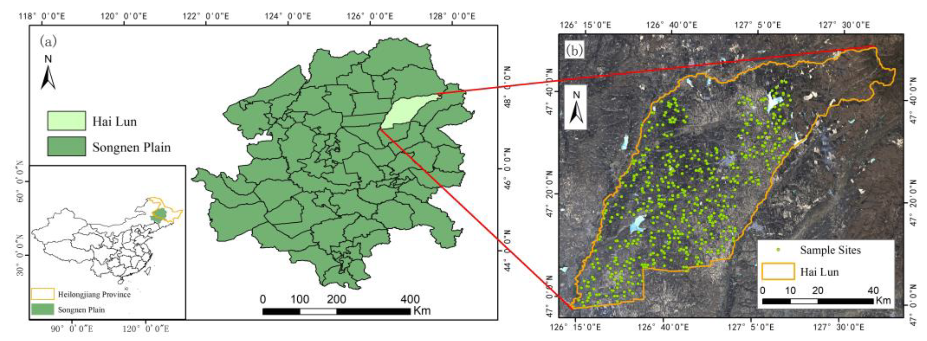
2.1. Study Area

The study area is located in Hai Lun City, Heilongjiang Province, northeast of China (46.961–47.838N, 126.221–127.749E), as shown in Figure 1a. The total area of it is 4667 km2. Hai Lun City lies on the northeast of Songnen Plain. The study area is the center of China’s black soil area. The average annual temperature in the study area was 1.5 °C, the annual rainfall was 500–600 mm, and the annual sunshine hours were 2600–2800 h. The dominant land use are cropland and woodland. Due to human activities, the region has undergone dynamic change in land use, and woodland has been constantly transformed into cropland. The meadow vegetation in the study area lasts about 6 months every year. During the rest of the year, the land use changed from meadow vegetation to bare soil, and the long duration and low temperature in winter severely limited the soil microbial activity. Therefore, the study area formed a deep black soil layer, and contains high content of soil humus. The main types of soil are Luvisols and Phaeozems, according to the Soil Taxonomy of World Reference Base (WRB) [35].

2.2. Sample Collection and Statistics

A total of 496 soil samples were collected in October 2013 at 0–15 cm. The distribution of the samples is shown in Figure 1b. All samples were put into sealed plastic sample bags and sent to the laboratory. After the soil samples were air-dried and the sundries are separated, let the soil samples pass through a 2 mm sieve until all the soil samples pass through the sieve hole. Soil organic carbon (SOC) content in soil samples was determined by the potassium dichromate volumetric method. The conversion factor of 1.724 was used to convert SOC content to SOM.
The reflectivity of soil is a cumulative property formed by the heterogeneous combination of different substances in soil, including organic matter. In this study, the SOM content of the collected samples covers a wide range, which can reflect the reflectivity of soil with different organic matter content. The 496 samples collected were arranged in ascending order. The first sample was selected, and then one sample was selected every three samples as the validation set, and the remaining samples were used as the training set. After the classification, the original sample set was divided into training set and validation set in a ratio of 3:1. The training set was used to build models, and the validation set was used to test the accuracy of models. The statistics of each sample set for SOM content were summarized in Table 1. The maximum and minimum SOM content of the training sample set are 4.73 and 0.69, respectively, and the maximum and minimum SOM content of the validation sample set are 4.45 and 0.49, respectively. The average values and the standard deviation of training sample set are essentially the same as those of validation sample set.

2.3. Spectral Measurement

The spectral data of the soil was collected in a dark laboratory using an ASD FieldSpec® 3 portable spectro-radiometer (Analytical Spectral Devices Inc., Boulder, CO, USA) with a spectral range of 350–2500 nm and a resample interval of 1 nm. The ground soil samples are put into a black container with a diameter of 10 cm and a depth of 2 cm. After filling, the surface of soil samples is scraped flat. A 50 W halogen lamp was used as the light source and the zenith Angle was 30°. The field of view Angle of the probe is set as 15°, and the distance from the probe to the surface of soil samples is 5 cm. Before each spectral determination, the whiteboard calibration was carried out. The spectrum was measured for 10 times repeatedly for each sample, and the average reflectance was taken as the actual spectral reflection data.

2.4. Preprocessing Methods

In order to reduce the influence of noise, marginal bands with low signal-noise ratio (350–400 nm and 2401–2500 nm) were eliminated before preprocessing. Various spectral preprocessing techniques were used in this study. First, spectral denoising includes four methods: none (N), Svitzky-Golay filter (SGF), multiplicative scatter correction (MSC), wavelet packet transform (WPT), as shown in Appendix A.1. After spectral denoising, fractional derivatives, FD and SD were used to process the spectrum, as shown in Appendix A.2. Then, spectral dimensionality reduction is carried out. Dimensionality reduction methods include principal component analysis (PCA), multidimensional scaling (MDS), locally linear embedding (LLE), as shown in Appendix A.3. All methods are listed in Table 2. In this study, the coefficient of determination ( R 2 ), root mean squared error (RMSE) and residual predictive deviation (RPD) of the validation set were used as the indicators to evaluate the model accuracy.

3. Results

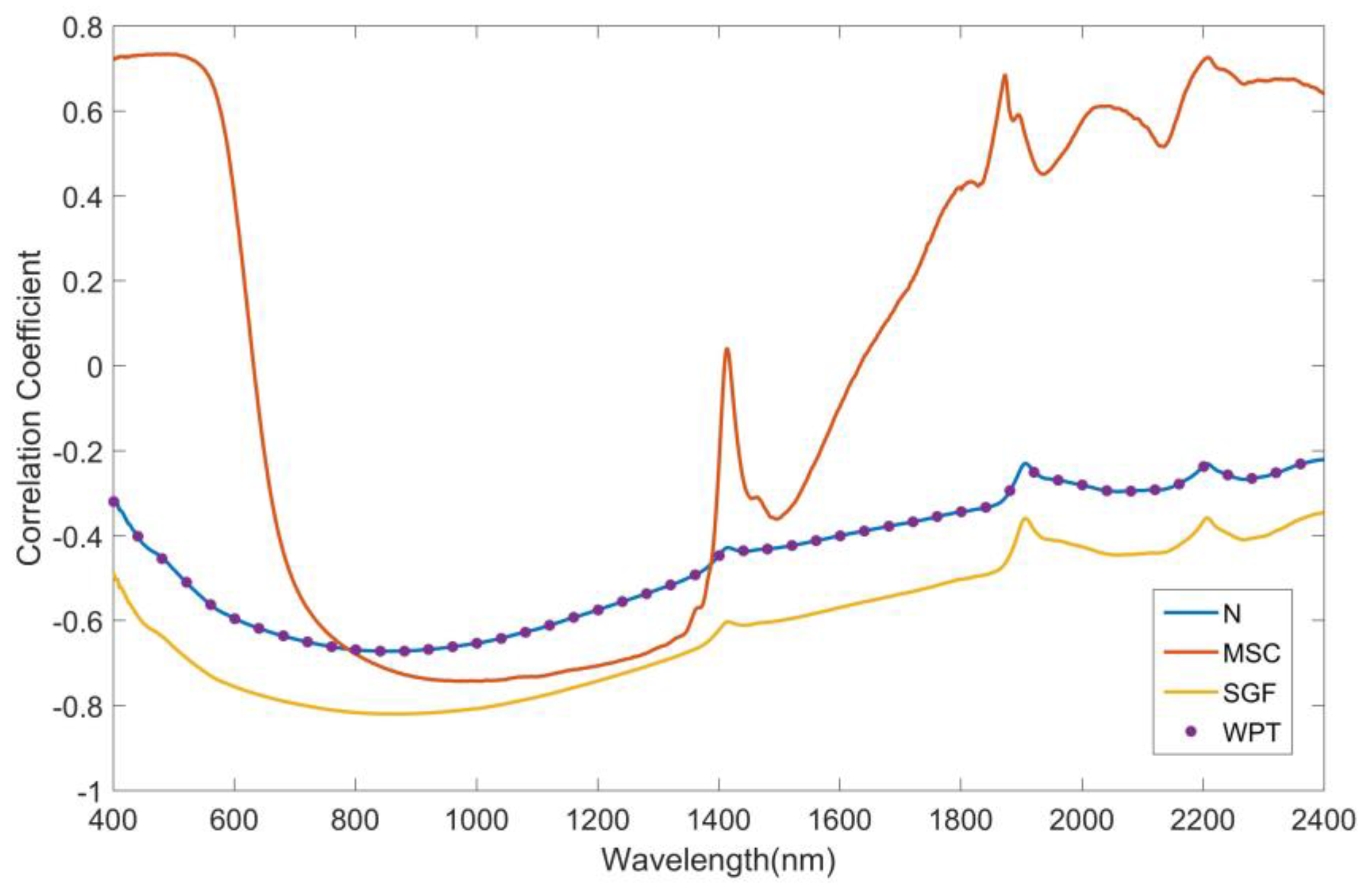
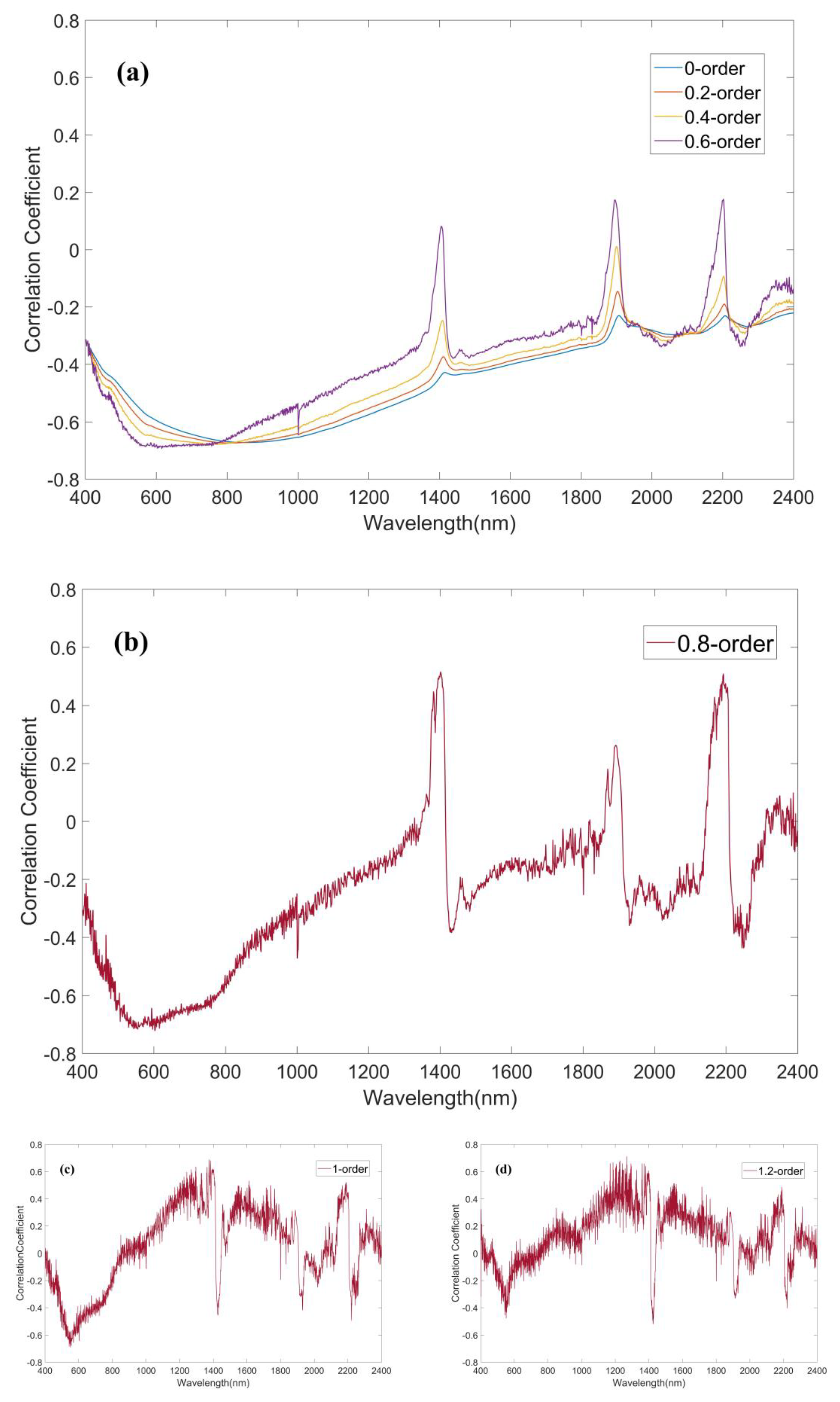
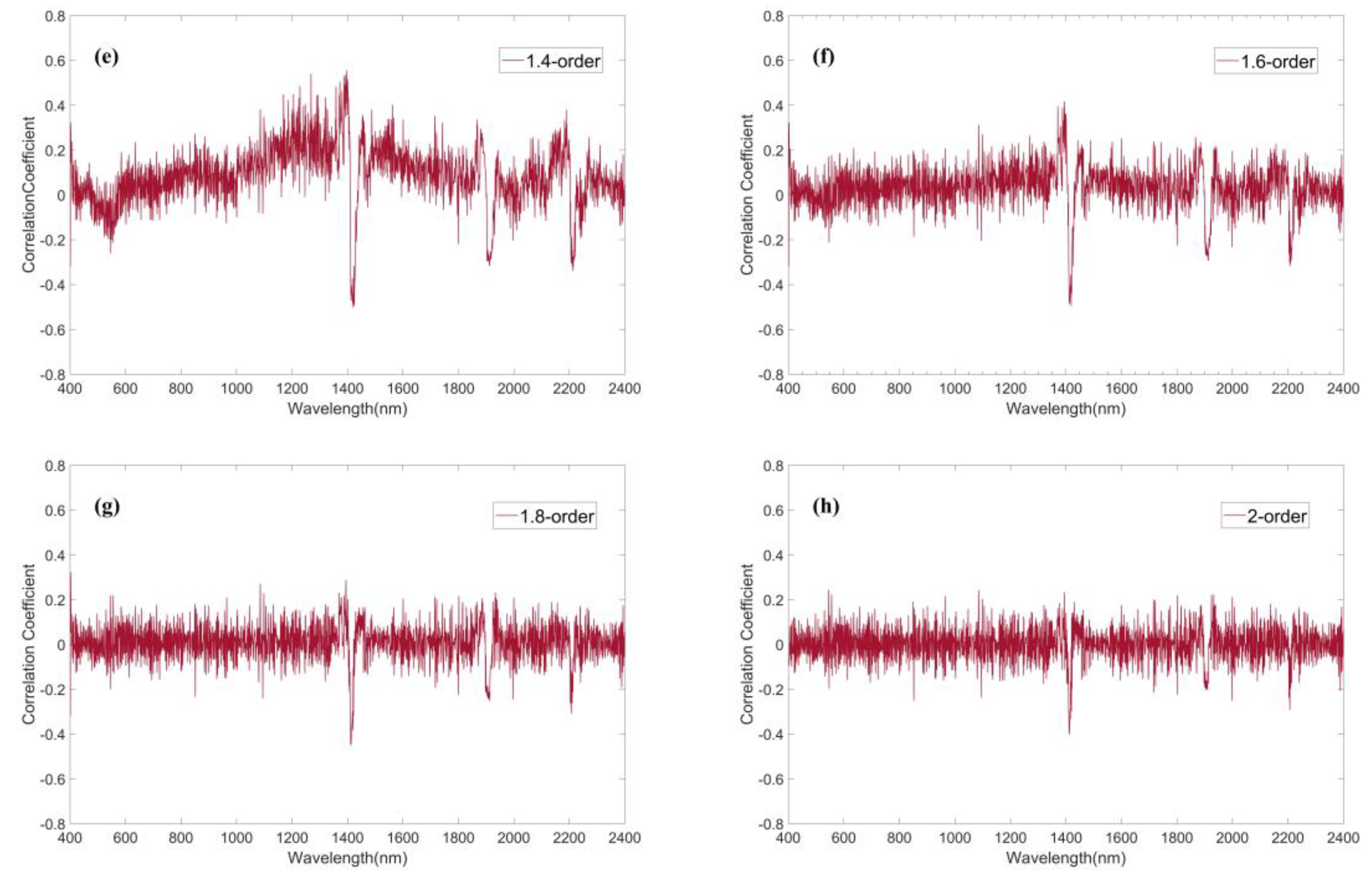
3.1. Correlation Analysis Between SOM Content and Reflectance Data

In this study, four different methods were used for denoising, including N, SGF, MSC, and WPT. Then, the data was processed with order 0 to 2 derivatives at 0.2 intervals. Finally, the dimensionality reduction was carried out for the data after derivatives, and then models were established. In order to observe the effect of denoising and fractional derivatives on the original spectrum, the correlation analysis between SOM content and reflectivity is conducted in the following two parts. The first part is the change of correlation curve after using different denoising methods. The second part is the change of the correlation curve after using derivatives of different orders.
Figure 2 shows the correlation curve between reflectance and SOM content after using different denoising methods. It can be seen that there is a negative correlation between the original reflectance and SOM content at 400–2400 nm. After WPT denoising, the correlation curve did not change obviously, and it basically coincides with the original correlation curve. The overall correlation coefficient of reflectance and SOM content after SGF improved about 0.2. The shape of the correlation curve is similar to the original correlation curve. Furthermore, the correlation between reflectance and SOM content after MSC denoising varied significantly between 400 nm and 2400 nm. The correlation curve shows a significant positive correlation between 400 nm and 577 nm (correlation coefficient > 0.6), followed by a rapid decline. Moreover, at 736–1354 nm, there is a significant negative correlation (correlation coefficient is less than −0.6), and then it fluctuates and rises, showing a more obvious positive correlation again.
The correlation curves between reflectance and SOM content after fractional derivatives are shown in Figure 3. As the order increases from 0 to 0.6, the region with high correlation in the correlation curve gradually moves to the visible range. At order 0, the band range with correlation coefficient greater than 0.5 is 514–1350 nm. At order 0.6, the band range with correlation coefficient greater than 0.5 is 446–1085 nm. From order 0 to 0.6, the peak of correlation coefficient increased from 0.6726 to 0.6934, and the band range with correlation coefficient greater than 0.67 moved from 807–905 nm to 539–787 nm. Starting from order 0.8, the correlation curve produces irregular fluctuations. As the order increases from 0.8 to 2, the fluctuation amplitude of the correlation curve increases rapidly, and the overall correlation coefficient tends to be between −0.2–0.2 gradually.

3.2. Accuracy Analysis of SOM Content Estimation Models

In this study, PCA, MDS, and LLE were used to reduce the dimension of the spectrum. For data that has been processed differently, the dimensions best suited for modeling are different. Therefore, the data after different processing was reduced to 0–200 dimensions. After dimensionality reduction, 0–200 dimensional models were established by partial least squares regression (PLSR) separately, the explanation of PLSR is shown in Appendix A.4, and the model with the largest R 2 is selected as the modeling result.
All SOM content estimation model results are shown in Appendix B. After PCA dimensionality reduction, the SOM content estimation model results are listed in Table A1. After MDS dimensionality reduction, the SOM content estimation model results are listed in Table A2. After LLE dimensionality reduction, the SOM content estimation model results are listed in Table A3.

3.2.1. Comparison of Modeling Results for Denoising Methods

The models without fractional derivatives are divided into three categories according to dimensionality reduction methods. The accuracy of the models is shown in Table 3. For models with PCA dimensionality reduction, R 2 and RPD of the model with SGF were 0.15 and 0.57 higher than that without denoising, R 2 and RPD of the model with MSC were 0.04 and 0.06 lower than that without denoising, and R 2 and RPD of the model with WPT were 0.07 and 0.17 higher than that without denoising. For models with MDS dimensionality reduction, R 2 and RPD of the model with SGF were 0.23 and 0.71 higher than that without denoising, R 2 and RPD of the model with MSC were 0.01 and 0.02 lower than that without denoising, and R 2 and RPD of the model with WPT were 0.08 and 0.15 higher than that without denoising. For models with LLE dimensionality reduction, R 2 and RPD of the model with SGF were 0.11 and 0.13 higher than that without denoising, R 2 and RPD of the model with MSC were 0.01 and 0.02 higher than that without denoising, and R 2 and RPD of the model with WPT were same as that without denoising. According to the above comparison, the best results were obtained using SGF.

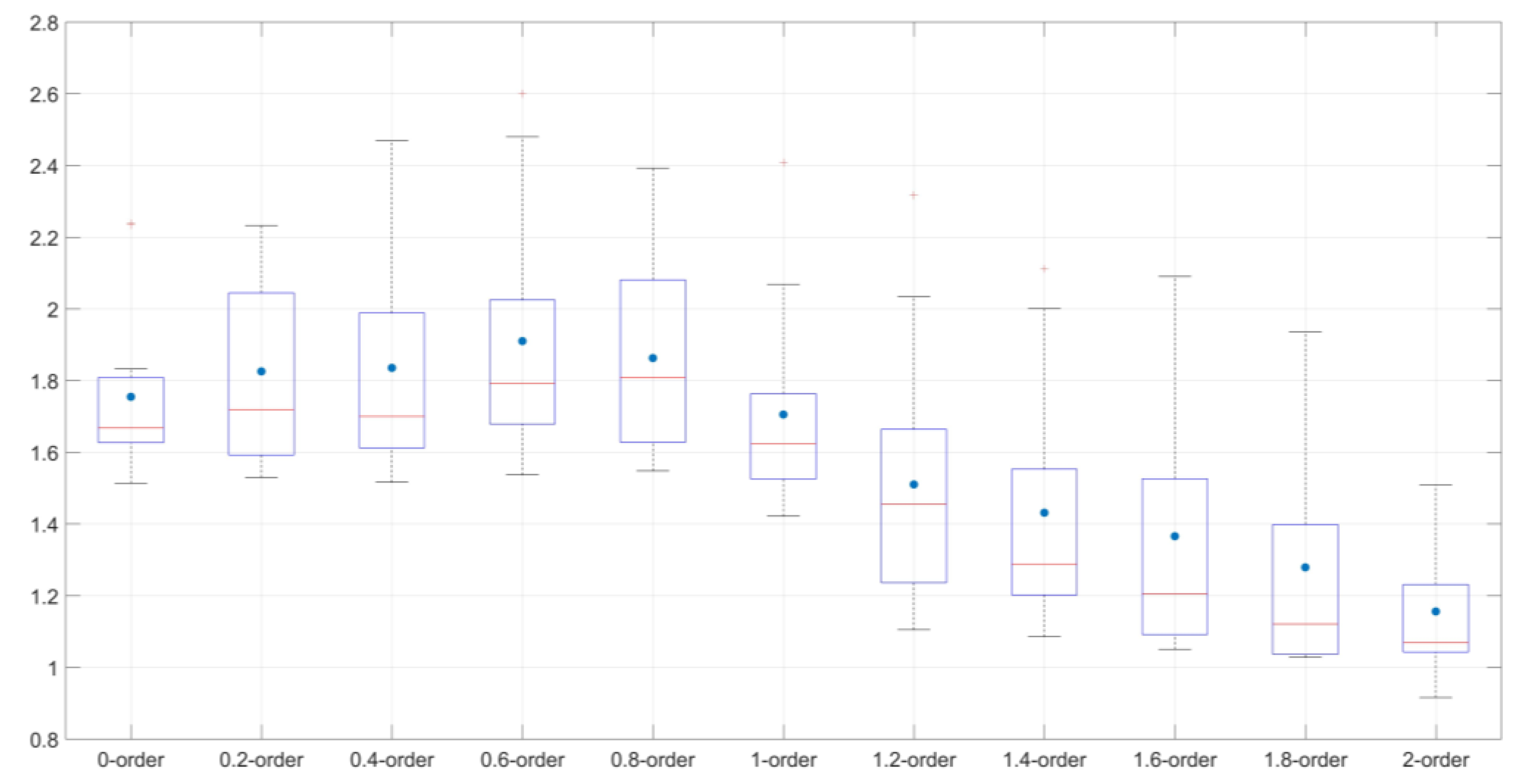
3.2.2. Comparison of Modeling Results for Fractional Derivatives of Different Orders

The models using the same denoising method and dimensionality reduction method were selected as a combination, and 12 combinations were formed. The RPD of models with 12 combinations were drawn in line charts, respectively (Figure 4). Among all models, RPD of the model after SGF-0.6 order-PCA achieved the maximum value of 2.60. The RPD of all combinations gradually decreased after first derivative, and the RPD of 8 combinations gradually decreased after 0.8 derivative. This is consistent with the change of the correlation curve between the reflectance and SOM content after fractional derivatives of different orders. 10 combinations obtained the maximum RPD at order 0.2–0.8, and two combinations obtained the maximum RPD at order 1. This indicates that the spectral data can show a more detailed variation trend after fractional derivative and reduce the accuracy decline caused by information loss.
The analyses of variance (ANOVA) was performed with RMSE as the dependent variable and with the fractional derivatives as the independent variable (Table 4). The result showed that fractional derivatives exerted large effect on the accuracy of the SOM content models ( p < 0.01 ). To further elucidate the effect of fractional derivatives, the RPD of SOM content estimation models using different order derivatives was counted to form the boxplot, as shown in Figure 5. The 0.2–0.8 derivatives improved the mean value, median value, and quartile of RPD. In addition, as the order increases from the first derivative, the accuracy of the models was reduced obviously.

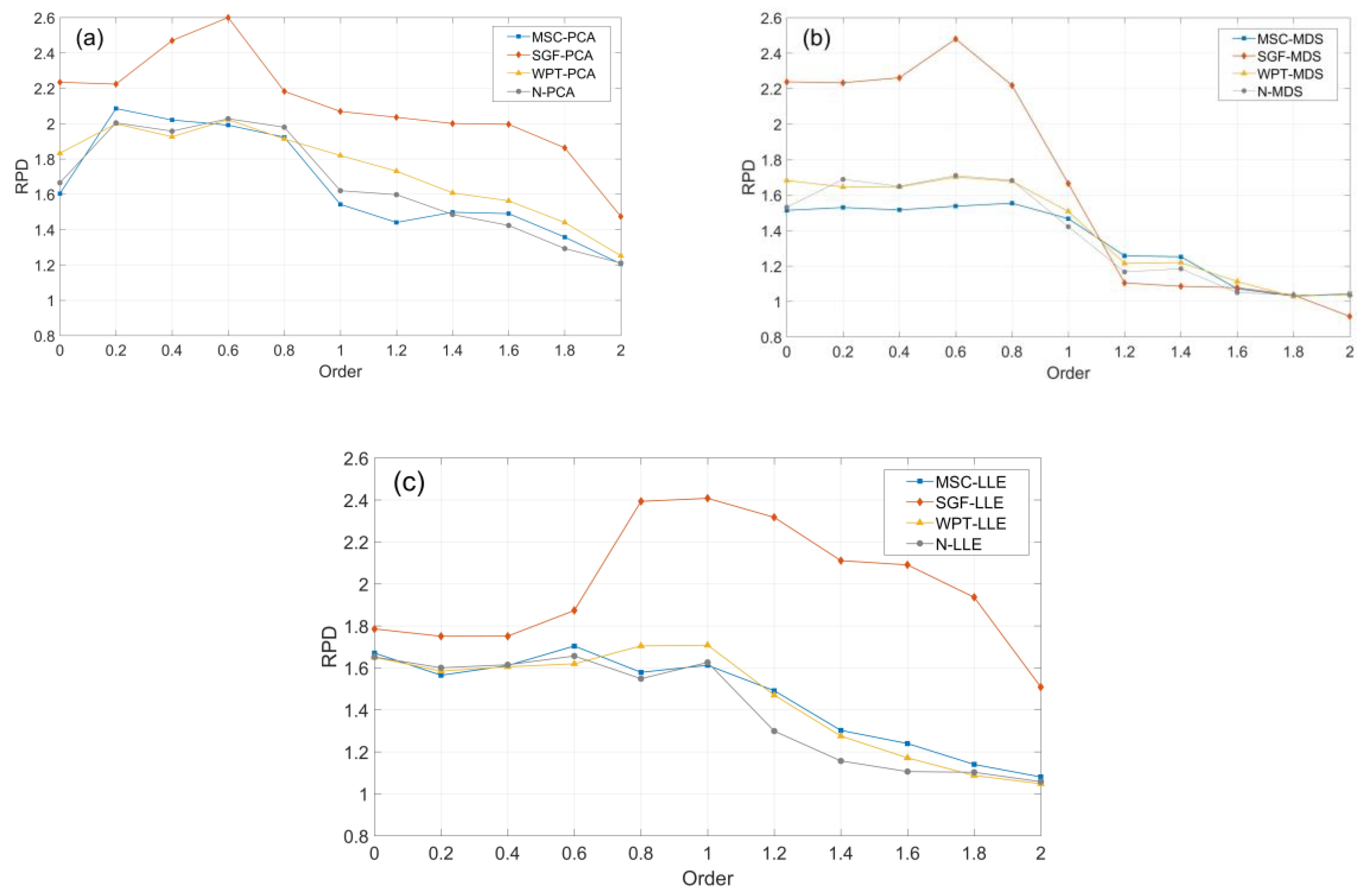
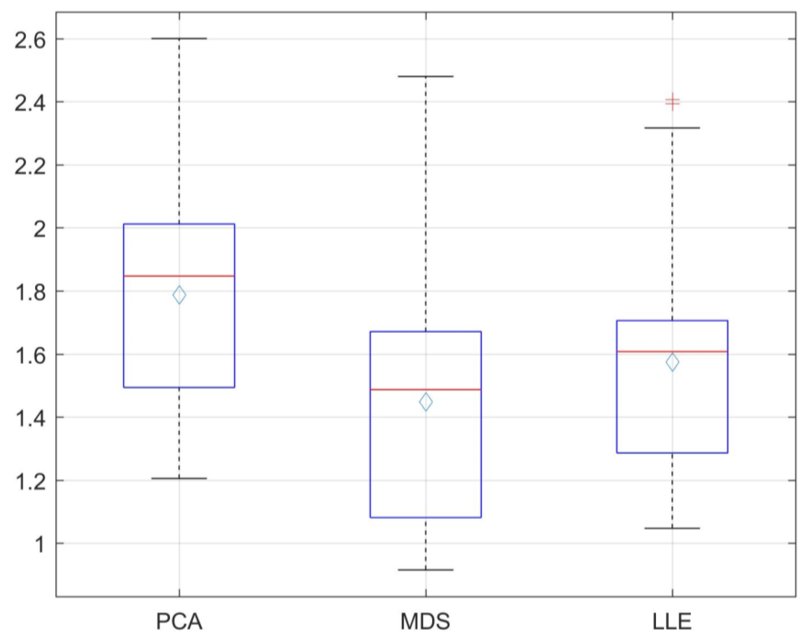
3.2.3. Comparison of Modeling Results for Dimensionality Reduction Methods

A total of 132 models are divided into three categories according to dimensionality reduction methods. The boxplot of RPD is shown in Figure 6. The mean RPD of the models with PCA dimensionality reduction method reached 1.79, which was 0.34 higher than that with MDS dimensionality reduction method, and 0.22 higher than that with LLE dimensionality reduction method. In addition, the quartile, maximum and minimum values of RPD of the models processed with PCA were significantly improved compared with those with MDS and LLE. There are two outliers in RPD of the models using LLE. Furthermore, the mean value and quartile of RPD of the models processed with LLE are greater than that with MDS. By comparing the MDS section and LLE section in the boxplot, the scope of the latter is smaller and more concentrated. This suggests that the accuracy fluctuation of the models processed with LLE is less.
Among the models with the same denoising method, derivative of the same order and different dimensionality reduction methods, the model achieving the largest RPD is denoted as the advantage model; 44 advantage models were obtained by statistics. The model achieving the largest RPD among the models with the same dimensionality reduction method is denoted as the optimal model. There were three optimal models were obtained by statistics. According to the statistical results, the table as shown in Table 5 is formed. Most of the advantage models come from models using PCA. In addition, the optimal model using PCA was 0.01 and 0.12 higher than that using MDS in R 2 and RPD and was 0.02 and 0.19 higher than that using LLE in R 2 and RPD.

4. Discussion

4.1. Denoising Methods for SOM Content Estimation in Black Soil Area

Different denoising methods have varied effects on the spectrum. In this study, N, SGF, MSC, and WPT were used. SGF can effectively remove noise such as baseline-drift, tilt, and reverse [36]. The larger the window size of SGF, the greater for spectral smoothing. This is because large window size can effectively remove high frequency noise [37], but the information loss will be caused using oversize window. MSC can be used to remove the effect of scattering on the spectrum [38]. WPT achieves the signal-noise separation by decomposing the low-frequency information and high-frequency noise in the spectrum [39]. With the same derivative order and dimensionality reduction method, the accuracy of most models using SGF is higher than that using the other three denoising methods. In Figure 2, the correlation curves between SOM content and reflectance shows that SGF can effectively improve the correlation, while the correlation curve after WPT basically coincides with the original correlation curve. The advantages of the SGF were not apparent in the results obtained by Shen et al. [25]. Determining appropriate smoothing window size was essential for removing noise and retain information of spectral data [37]. In the study of Shen et al., the smoothing window of 22 was selected, which might cause over-smoothing phenomenon. Furthermore, MSC has little effect on SOM content estimation according to model accuracy variation. Before spectral measurement, the sundries and large particles in samples have been separated. Therefore, the influence of inhomogeneous scattering on the spectrum is not significant, and MSC has less effect. For the field measured spectrum of soil, due to the presence of impurities, MSC might achieve better performance in SOM content estimation, which requires further study.

4.2. Fractional Derivatives for SOM Content Estimation in Black Soil Area

SOM content has a key effect on soil reflectivity [40]. Several studies have reported that SOM content is strongly correlated to the reflectance in visible region [41,42,43,44]. In addition, the results obtained by Peng et al. showed that 570–630 nm spectrum were more significantly affected by SOM through comparing the soil reflectance before and after the removal of SOM [45]. In the study, according to the statistics of original spectrum, the band range with correlation coefficient greater than 0.5 is 514–1350 nm. After 0.6 order derivative of the spectrum, the band range with correlation coefficient greater than 0.5 moves to 446–1085 nm, and peaks of correlation shift to the visible range significantly. Moreover, the peak of correlation coefficient increased from 0.67 to 0.69 and the band range with correlation coefficient greater than 0.67 moves from 807–905 nm to 539–787 nm. The range of SOM sensitive bands after 0.6 order derivative of spectrum in this study is consistent with previous studies [41,42,43,44,45]. This indicates that fractional derivatives can accentuate spectral features of SOM. It is significant for SOM content estimation using Vis–NIR spectroscopy.
In Figure 3, the study compares the change of the correlation curve between the original spectrum after fractional derivatives and SOM content. By observing Figure 3, it can be seen that the correlation curve between the spectrum and SOM content has shown slight irregular fluctuation at order 0.8, and the irregular fluctuation becomes more obvious at order 1.2. As the order goes up, an increasing number of noise is introduced to the correlation curve, causing the correlation decreases.
Figure 4 shows the variation of model accuracy after fractional derivatives among 12 combinations of preprocessing techniques. In most combinations, the commonly used FD and SD cannot significantly improve the model accuracy. After SD, the accuracy of the models is lower than that without derivative. This is related to the noise introduced by SD while separating the absorption peak. Moreover, the spectrum after FD and SD forms obvious sharp peaks [25]. Among 12 combinations, 10 combinations achieved the optimal performance at order 0.2–0.8. In addition, Figure 5 showed that 0.2–0.8 order derivatives could improve accuracy of the models. In previous studies, the optimal results of SOM content estimation were obtained at 0.25-order in the southeast part of Iowa State [15], 1.25-order and 1.5-order in the east of Jianghan plain (Hubei Province, China) [29], and 1.2-order in Ebinur Lake Wetland National Nature Reserve (Xinjiang, China) [30]. Because soil types varied in different study areas, the appropriate orders for SOM content estimation might be different. Therefore, 0.2–0.8 order derivatives have more advantages in hyperspectral SOM content estimation in black soil area, especially 0.6 order and 0.8 order. Moreover, refinement of the order variation of fractional derivatives to order 0.1 or lower may further improve the modeling effect. The influence of refining the order variation of fractional derivatives on hyperspectral SOM content estimation needs to be further studied.

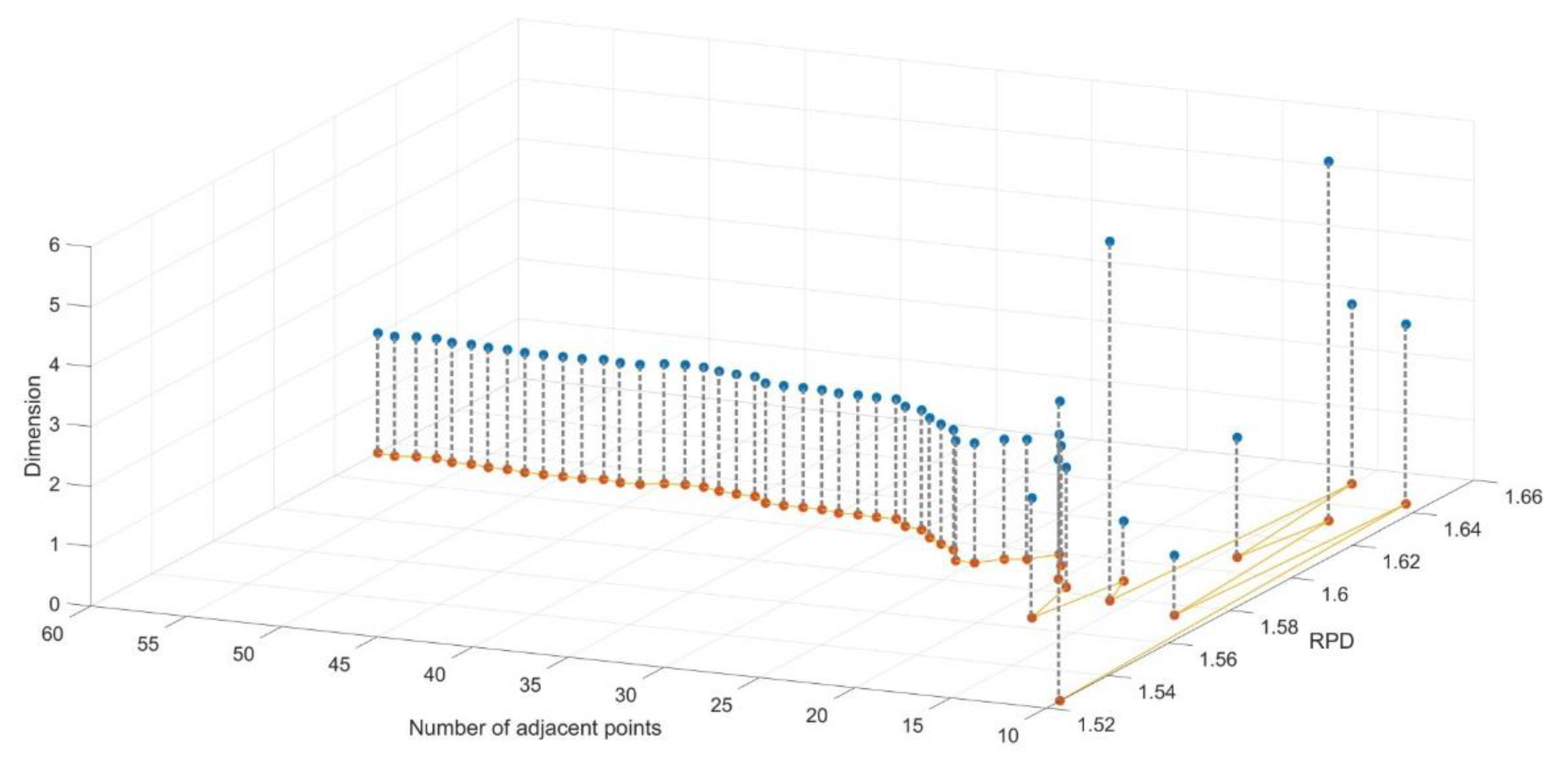
4.3. Dimensionality Reduction Methods for SOM Content Estimation in Black Soil Area

In this study, PCA, MDS, and LLE were used for dimensionality reduction. It can be concluded from Figure 6 that PCA achieves the optimal performance in each evaluation index compared with the other two methods. In addition, Table 5 shows that most advantage models come from models using PCA. Among three optimal models, the model using PCA achieves the highest accuracy and 31 of 44 advantage models come from the models using PCA. Compared with PCA, MDS, and LLE did not show superiority in SOM content estimation. This is related with the characteristic of the three dimensionality methods. PCA as a linear dimensionality reduction method is more adaptive for the dependent variables with a linear relation to the reflectance [31]. There is obvious trend on soil reflectance when SOM content varies. The reflectivity of soil decreases as the increase of SOM content [40]. In the case that the relation between the reflectance and the dependent variable is not significant, LLE and MDS are more applicable [31]. Therefore, LLE and MDS might achieve better performance in estimating the content of other components in the soil, which requires further study.

5. Conclusions

In this study, the spectral data of 496 soil samples was preprocessed in three parts: denoising, fractional derivatives and dimensionality reduction, and PLSR was used for modeling. A total of 132 models using combinations of different preprocessing techniques were obtained. Compared with MSC and WPT, SGF can enhance the correlation between soil spectrum and SOM content more effectively. In addition, the advantages of the SGF were apparent in improving the accuracy of SOM content estimation. The use of low-order fractional derivatives can accentuate spectral features of SOM, causing the correlation peak increasing, the bands around the correlation peak moving to visible range, and the number of bands around the correlation peak increasing. However, as the order increasing from 0.8, the spectrum was susceptible to spectral noise interferences. The results indicated that the 0.2–0.8 order derivatives significantly enhanced the accuracy of the SOM content estimation models. Among dimensionality reduction methods, PCA exhibited better performance than LEE and MDS.
According to this study, for three categories of preprocessing techniques, we found that SGF, 0.2–0.8 order derivative and PCA are appropriate methods to estimate SOM content in black soil area. Despite the above conclusion has been drawn, SOM content estimation in black soil area remains to be further studied. In the future, the researches should be focus on spectrum at different scales (e.g., unmanned aerial vehicle hyperspectral image, and satellite hyperspectral image), in order to improve the efficiency and accuracy of SOM content estimation in black soil area.

Author Contributions

All of the authors contributed to the study. X.X. conceived and designed the experiments, analyzed the data, and wrote the manuscript. X.X., S.Z., and R.D. processed the data. Z.X. contributed greatly to data collection. S.C. and Y.Y. reviewed the manuscript. All authors have read and agreed to the published version of the manuscript.

Funding

This research was funded by Jilin province and Jilin university co-building project (Grant No. SXGJXX2017-2) and the program for JLU science and technology innovative research team (Grant No. JLUSTIRT, 2017TD-26).

Acknowledgments

We thank the editors and the reviewers for their constructive suggestions and insightful comments, which helped us greatly to improve this manuscript.

Conflicts of Interest

The authors declare no conflict of interest.

Appendix A

Appendix A.1. Denoising Methods

SGF removes the high frequency noise points by the least square fitting to internal elements of moving window and replacing the original value with the fitting value [46]. SGF can not only achieve expected denoising effect, but also retain useful information in the spectrum [47]. Therefore, SGF is often used in the preprocessing of spectral data. The method has two parameters, filter window size and polynomial fitting order. The higher the polynomial fitting order, the more details are retained, and the larger the window size, the better the smoothing effect [48]. In this study, the filter window size is 15 and the polynomial fitting order is two.
MSC corrected the difference of scattering information in different sample spectrum to the same level to minimize the interference information independent of sample composition caused by spectral scattering [49]. Therefore, the main purpose of MSC is to remove the influence caused by scattering [50]. MSC calculates the n × p dimension matrix of the sample set, where n is the number of samples and p is the number of bands. Formulas (A1), (A2) and (A3) are used for calculation.
x ¯ i , j = i = 1 n A i , j n
x i = m i x ¯ i , j + b i
x i ( M S C ) = ( x i b i ) / m i
where n is the number of samples, i and j respectively represent the i sample and the j band, and x ¯ i , j represents the average spectrum of all samples in each band. m i represents the relative offset coefficient of each sample spectrum, and b i represents the translation variable of each sample spectrum.
Wavelet packet transform is proposed on the basis of wavelet transform. Wavelet packet transform can achieve more accurate information extraction through further decomposing the high frequency information. Wavelet packet transform has been widely used in various fields related to signal processing [39,51]. Wavelet packet denoising consists of four parts: wavelet packet decomposition, optimal wavelet packet basis function determination, threshold selection, and signal wavelet packet reconstruction. In this study, db2 wavelet basis function was selected to perform two-layer wavelet packet decomposition for the spectrum. The use of hard threshold processing may cause the reconstructed signal to vibrate [52]. Therefore, the continuous soft threshold function is selected, and then the signal is reconstructed by wavelet packet transform. The threshold value is calculated by formula (A4):
t a r = σ 2 log e N
where σ is the median of all absolute coefficients in the high-frequency signal divided by 0.6745, N is the number of data in the high-frequency signal, and t a r / 2 is selected as the denoising threshold [22].

Appendix A.2. Fractional Derivative

Fractional derivatives extend the concept of integer derivatives and have been applied to image processing [53], fractal theory [54], and other fields. There are three main expressions of fractional derivatives: Riemann Liouville (R-L), Grunwald–Letnikov (G-L), and Caputo [55,56]. Due to the uncomplicated formula of G-L and the simple coefficient, G-L is often used in signal processing [57]. The fractional derivatives of function f ( x ) is shown in formula (A5) [30]:
d v f ( x ) d x v f ( x ) + ( v ) f ( x 1 ) + ( v ) ( v + 1 ) 2 f ( x 2 ) + + Γ ( v + 1 ) n ! Γ ( v + n + 1 ) f ( x n )
where v is the order.

Appendix A.3. Dimensionality Reduction Methods

Principal component analysis (PCA) is the most widely used linear dimensionality reduction technique. PCA is a second order method based on covariance matrix. For PCA, dimensionality reduction is achieved by coordinate transformation. Coordinate transformation is to project high-dimensional data to the direction with the greatest variance and satisfy the conditions of minimum error and maximum variance simultaneously [58]. Each principal component obtained through PCA is independent of each other. Therefore, PCA can achieve dimensionality reduction and solve the problem of information redundancy in spectral data.
Multidimensional scaling (MDS) is a nonlinear analysis method that measures distance and reflects the anisotropy between data points. MDS was first proposed by Torgerson [59]. Torgerson converts the difference of things evaluated by different people into target distance. According to this, points are drawn in the figure to make the distance between points fit the target distance. Kruskal improved Torgerson’s approach [60]. The improved method is now the basis of MDS research. The main idea of MDS dimensionality reduction is to map the observed data in high dimensional space to low dimensional space. After mapping, Euclidean distance between two points should be kept unchanged as far as possible to keep the difference of samples in the low-dimensional space unchanged.
Local linear embedding (LLE) is a local feature preserving algorithm. LLE is a kind of manifold learning. The basic idea is to assume that each sample point and its neighbor point in a high dimensional space are located in a local neighborhood of a linear manifold. Under this assumption, each point can be represented linearly by an adjacent point. The reconstruction weight is obtained by minimizing the reconstruction error. Then the corresponding internal low-dimensional space coordinate representation is obtained by keeping the same reconstruction weight, and achieve the effect of dimensionality reduction [61,62,63]. When LLE is used to process spectral data, the number of adjacent points and dimension has great influence on dimensionality reduction results and model accuracy [33,34]. Therefore, in order to determine the number of adjacent points, the number of adjacent points is set from 10 to 60, and the range of dimensionality reduction is set from 0 to 200. With this setting, the original spectral data was used for modeling. According to model accuracy, the number of adjacent points was selected. Figure A1 shows the model accuracy curve. When the number of adjacent points is 15, the model accuracy reaches the maximum value. Therefore, in this study, the number of adjacent points of LLE was taken as 15.
Figure A1. Number of adjacent points in different dimension number versus RPD. The dimension number is determined by the dimension corresponding to the optimal RPD among 0–200 dimensions in the case that the number of adjacent points is the same.
Remotesensing 12 03765 g0a1

Appendix A.4. Partial Least Squares Regression (PLSR)

The conventional multiple linear regression methods face the problem of multi-collinearity among variables. PLSR integrates the advantages of principal component analysis, canonical correlation analysis and linear regression analysis. Because of the characteristic, PLSR can avoid the problem of strong correlation between variables, and fully extract effective information of samples [64]. It can be seen that PLSR is able to reveal the dominant band of soil chemical variable change from the spectral data and achieve regression modeling, so that PLSR is potential for spectral information mining. Moreover, PLSR is suitable for linear regression modeling of multi-dependent variables and multi-independent variables [65]. Therefore, PLSR has been widely used to find the correlation between soil spectrum and SOM [22,25,66].

Appendix B

The results of 132 models are divided into three parts depending on the dimensionality reduction method, as shown in Table A1, Table A2 and Table A3.
Table A1. SOM Content Estimation Model Results through PCA dimensionality reduction.
Denoising MethodsOrderR2RMSERPDDenoising MethodsOrderR2RMSERPD
MSC00.610.401.60SGF00.800.292.23
0.20.780.312.080.20.800.292.22
0.40.770.322.020.40.830.262.47
0.60.780.321.990.60.850.252.60
0.80.750.331.920.80.790.292.18
10.640.421.5410.760.312.07
1.20.590.451.441.20.760.322.04
1.40.560.431.501.40.750.322.00
1.60.550.431.491.60.750.322.00
1.80.510.471.361.80.710.341.86
20.310.531.2120.540.441.47
WPT00.720.351.83N00.650.391.66
0.20.770.322.000.20.770.322.00
0.40.760.331.920.40.780.331.96
0.60.790.322.020.60.800.322.03
0.80.770.341.910.80.760.321.98
10.730.351.8210.680.401.62
1.20.670.371.731.20.620.401.60
1.40.630.401.611.40.570.431.48
1.60.590.411.561.60.540.451.42
1.80.520.451.441.80.400.501.29
20.360.511.2520.310.531.21
Note: R 2 , coefficient of determination; RMSE, root mean squared error; RPD, residual predictive deviation; MSC, multiplicative scatter correction; SGF, Svitzky–Golay filter; WPT, wavelet packet transform; N, none.
Table A2. SOM Content Estimation Model Results through MDS dimensionality reduction.
Denoising MethodsOrderR2RMSERPDDenoising MethodsOrderR2RMSERPD
MSC00.560.421.51SGF00.800.292.24
0.20.580.421.530.20.800.292.23
0.40.570.421.520.40.800.282.26
0.60.580.421.540.60.840.262.48
0.80.590.411.550.80.800.292.22
10.530.441.4710.640.391.66
1.20.360.511.261.20.180.581.10
1.40.360.511.251.40.150.591.09
1.60.120.601.071.60.140.601.08
1.80.050.621.031.80.060.621.04
20.080.621.0420.080.700.92
WPT00.650.381.68N00.570.421.53
0.20.630.391.650.20.650.381.69
0.40.630.391.650.40.630.391.65
0.60.650.381.700.60.660.381.71
0.80.650.381.680.80.660.381.68
10.560.431.5110.500.451.42
1.20.320.531.211.20.260.551.17
1.40.330.531.221.40.280.541.18
1.60.200.581.111.60.120.611.05
1.80.060.621.031.80.070.621.04
20.080.621.0420.070.621.03
Note: R 2 , coefficient of determination; RMSE, root mean squared error; RPD, residual predictive deviation; MSC, multiplicative scatter correction; SGF, Svitzky–Golay filter; WPT, wavelet packet transform; N, none.
Table A3. SOM Content Estimation Model Results through LLE dimensionality reduction.
Denoising MethodsOrderR2RMSERPDDenoising MethodsOrderR2RMSERPD
MSC00.640.381.67SGF00.740.361.78
0.20.600.411.560.20.730.371.75
0.40.620.401.610.40.730.371.75
0.60.660.381.700.60.770.341.87
0.80.600.411.580.80.830.272.39
10.620.401.6110.830.272.41
1.20.550.431.491.20.820.282.32
1.40.410.491.301.40.800.302.11
1.60.340.521.241.60.780.312.09
1.80.230.561.141.80.730.331.94
20.140.591.0820.560.431.51
WPT00.630.391.65N00.630.391.65
0.20.610.411.580.20.610.401.60
0.40.610.401.600.40.620.401.61
0.60.620.401.620.60.640.391.66
0.80.660.381.700.80.580.411.55
10.660.381.7110.620.391.63
1.20.540.441.471.20.400.491.30
1.40.380.501.271.40.250.561.16
1.60.270.551.171.60.180.581.11
1.80.150.591.091.80.170.581.10
20.110.611.0520.120.611.06
Note: R 2 , coefficient of determination; RMSE, root mean squared error; RPD, residual predictive deviation; MSC, multiplicative scatter correction; SGF, Svitzky–Golay filter; WPT, wavelet packet transform; N, none.

References

  1. Zeraatpisheh, M.; Bakhshandeh, E.; Hosseini, M.; Alavi, S.M. Assessing the effects of deforestation and intensive agriculture on the soil quality through digital soil mapping. Geoderma 2020, 363, 114139. [Google Scholar] [CrossRef]
  2. Abdalla, M.; Hastings, A.; Chadwick, D.; Jones, D.; Evans, C.; Jones, M.B.; Rees, R.; Smith, P. Critical review of the impacts of grazing intensity on soil organic carbon storage and other soil quality indicators in extensively managed grasslands. Agric. Ecosyst. Environ. 2018, 253, 62–81. [Google Scholar] [CrossRef] [PubMed] [Green Version]
  3. Schillaci, C.; Acutis, M.; Lombardo, L.; Lipani, A.; Fantappie, M.; Märker, M.; Saia, S. Spatio-temporal topsoil organic carbon mapping of a semi-arid Mediterranean region: The role of land use, soil texture, topographic indices and the influence of remote sensing data to modelling. Sci. Total Environ. 2017, 601, 821–832. [Google Scholar] [CrossRef] [PubMed]
  4. Aldana-Jague, E.; Heckrath, G.; Macdonald, A.; van Wesemael, B.; Van Oost, K. UAS-based soil carbon mapping using VIS-NIR (480–1000 nm) multi-spectral imaging: Potential and limitations. Geoderma 2016, 275, 55–66. [Google Scholar] [CrossRef]
  5. Mirzaee, S.; Ghorbani-Dashtaki, S.; Mohammadi, J.; Asadi, H.; Asadzadeh, F. Spatial variability of soil organic matter using remote sensing data. Catena 2016, 145, 118–127. [Google Scholar] [CrossRef]
  6. Nabiollahi, K.; Taghizadeh-Mehrjardi, R.; Kerry, R.; Moradian, S. Assessment of soil quality indices for salt-affected agricultural land in Kurdistan Province, Iran. Ecol. Indic. 2017, 83, 482–494. [Google Scholar] [CrossRef]
  7. Han, X.; Li, N. Research progress of Black soil in Northeast China. Sci. Geogr. Sin. 2018, 38, 1032–1041. [Google Scholar]
  8. Liu, X.; Zhang, X.; Wang, Y.; Sui, Y.; Zhang, S.; Herbert, S.; Ding, G. Soil degradation: A problem threatening the sustainable development of agriculture in Northeast China. Plant Soil Environ. 2010, 56, 87–97. [Google Scholar] [CrossRef] [Green Version]
  9. Castaldi, F.; Palombo, A.; Santini, F.; Pascucci, S.; Pignatti, S.; Casa, R. Evaluation of the potential of the current and forthcoming multispectral and hyperspectral imagers to estimate soil texture and organic carbon. Remote Sens. Environ. 2016, 179, 54–65. [Google Scholar] [CrossRef]
  10. Bao, N.; Wu, L.; Ye, B.; Yang, K.; Zhou, W. Assessing soil organic matter of reclaimed soil from a large surface coal mine using a field spectroradiometer in laboratory. Geoderma 2017, 288, 47–55. [Google Scholar] [CrossRef]
  11. Cambou, A.; Cardinael, R.; Kouakoua, E.; Villeneuve, M.; Durand, C.; Barthès, B.G. Prediction of soil organic carbon stock using visible and near infrared reflectance spectroscopy (VNIRS) in the field. Geoderma 2016, 261, 151–159. [Google Scholar] [CrossRef] [Green Version]
  12. Vašát, R.; Kodešová, R.; Borůvka, L.; Klement, A.; Jakšík, O.; Gholizadeh, A. Consideration of peak parameters derived from continuum-removed spectra to predict extractable nutrients in soils with visible and near-infrared diffuse reflectance spectroscopy (VNIR-DRS). Geoderma 2014, 232, 208–218. [Google Scholar] [CrossRef]
  13. Ben-Dor, E.; Banin, A. Near-infrared analysis as a rapid method to simultaneously evaluate several soil properties. Soil Sci. Soc. Am. J. 1995, 59, 364–372. [Google Scholar] [CrossRef]
  14. Ben-Dor, E.; Irons, J.; Epema, G. Soil reflectance. Remote Sens. Earth Sci. Man. Remote Sens. 1999, 3, 111–188. [Google Scholar]
  15. Hong, Y.; Guo, L.; Chen, S.; Linderman, M.; Mouazen, A.M.; Yu, L.; Chen, Y.; Liu, Y.; Liu, Y.; Cheng, H. Exploring the potential of airborne hyperspectral image for estimating topsoil organic carbon: Effects of fractional-order derivative and optimal band combination algorithm. Geoderma 2020, 365, 114228. [Google Scholar] [CrossRef]
  16. Hong, Y.; Liu, Y.; Chen, Y.; Liu, Y.; Yu, L.; Liu, Y.; Cheng, H. Application of fractional-order derivative in the quantitative estimation of soil organic matter content through visible and near-infrared spectroscopy. Geoderma 2019, 337, 758–769. [Google Scholar] [CrossRef]
  17. Gholizadeh, A.; Borůvka, L.; Saberioon, M.; Vašát, R. Visible, near-infrared, and mid-infrared spectroscopy applications for soil assessment with emphasis on soil organic matter content and quality: State-of-the-art and key issues. Appl. Spectrosc. 2013, 67, 1349–1362. [Google Scholar] [CrossRef]
  18. Rinnan, Å.; Van Den Berg, F.; Engelsen, S.B. Review of the most common pre-processing techniques for near-infrared spectra. TrAC Trends Anal. Chem. 2009, 28, 1201–1222. [Google Scholar] [CrossRef]
  19. Vohland, M.; Bossung, C.; Fründ, H.C. A spectroscopic approach to assess trace–heavy metal contents in contaminated floodplain soils via spectrally active soil components. J. Plant Nutr. Soil Sci. 2009, 172, 201–209. [Google Scholar] [CrossRef]
  20. Candolfi, A.; De Maesschalck, R.; Jouan-Rimbaud, D.; Hailey, P.; Massart, D. The influence of data pre-processing in the pattern recognition of excipients near-infrared spectra. J. Pharm. Biomed. Anal. 1999, 21, 115–132. [Google Scholar] [CrossRef]
  21. Wei, L.; Yuan, Z.; Wang, Z.; Zhao, L.; Zhang, Y.; Lu, X.; Cao, L. Hyperspectral Inversion of Soil Organic Matter Content Based on a Combined Spectral Index Model. Sensors 2020, 20, 2777. [Google Scholar] [CrossRef] [PubMed]
  22. Liu, Y.; Liu, Y.; Chen, Y.; Zhang, Y.; Shi, T.; Wang, J.; Hong, Y.; Fei, T. The influence of spectral pretreatment on the selection of representative calibration samples for soil organic matter estimation using Vis-NIR reflectance spectroscopy. Remote Sens. 2019, 11, 450. [Google Scholar] [CrossRef] [Green Version]
  23. Gao, Y.; Cui, L.; Lei, B.; Zhai, Y.; Shi, T.; Wang, J.; Chen, Y.; He, H.; Wu, G. Estimating soil organic carbon content with visible-near-infrared (Vis-NIR) spectroscopy. Appl. Spectrosc. 2014, 68, 712–722. [Google Scholar] [CrossRef] [PubMed]
  24. Nawar, S.; Buddenbaum, H.; Hill, J.; Kozak, J.; Mouazen, A.M. Estimating the soil clay content and organic matter by means of different calibration methods of vis-NIR diffuse reflectance spectroscopy. Soil Tillage Res. 2016, 155, 510–522. [Google Scholar] [CrossRef] [Green Version]
  25. Shen, L.; Gao, M.; Yan, J.; Li, Z.-L.; Leng, P.; Yang, Q.; Duan, S.-B. Hyperspectral Estimation of Soil Organic Matter Content using Different Spectral Preprocessing Techniques and PLSR Method. Remote Sens. 2020, 12, 1206. [Google Scholar] [CrossRef] [Green Version]
  26. Wiggins, K.; Palmer, R.; Hutchinson, W.; Drummond, P. An investigation into the use of calculating the first derivative of absorbance spectra as a tool for forensic fibre analysis. Sci. Justice 2007, 47, 9–18. [Google Scholar] [CrossRef]
  27. Peng, X.; Shi, T.; Song, A.; Chen, Y.; Gao, W. Estimating soil organic carbon using VIS/NIR spectroscopy with SVMR and SPA methods. Remote Sens. 2014, 6, 2699–2717. [Google Scholar] [CrossRef] [Green Version]
  28. Kharintsev, S.; Salakhov, M.K. A simple method to extract spectral parameters using fractional derivative spectrometry. Spectrochim. Acta Part A Mol. Biomol. Spectrosc. 2004, 60, 2125–2133. [Google Scholar] [CrossRef]
  29. Hong, Y.; Chen, Y.; Yu, L.; Liu, Y.; Liu, Y.; Zhang, Y.; Liu, Y.; Cheng, H. Combining fractional order derivative and spectral variable selection for organic matter estimation of homogeneous soil samples by VIS–NIR spectroscopy. Remote Sens. 2018, 10, 479. [Google Scholar] [CrossRef] [Green Version]
  30. Wang, X.; Zhang, F.; Johnson, V.C. New methods for improving the remote sensing estimation of soil organic matter content (SOMC) in the Ebinur Lake Wetland National Nature Reserve (ELWNNR) in northwest China. Remote Sens. Environ. 2018, 218, 104–118. [Google Scholar] [CrossRef]
  31. Bengio, Y.; Delalleau, O.; Le Roux, N.; Paiement, J.-F.; Vincent, P.; Ouimet, M. Spectral Dimensionality Reduction. In Feature Extraction: Foundations and Applications; Guyon, I., Nikravesh, M., Gunn, S., Zadeh, L.A., Eds.; Springer: Berlin/Heidelberg, Germany, 2006; pp. 519–550. [Google Scholar]
  32. Machado, J.T.; Dinç, E.; Baleanu, D. Analysis of UV spectral bands using multidimensional scaling. Signal Image Video Process. 2015, 9, 573–580. [Google Scholar] [CrossRef] [Green Version]
  33. Duan, Y.; Wang, Q.; Ma, M.; Lu, X.; Wang, C. Study on non-destructive detection method for egg freshness based on LLE-SVR and visible/near-infrared spectrum. Spectrosc. Spectr. Anal. 2016, 36, 981–985. [Google Scholar]
  34. Ya-chun, M.; Rui-bo, D.; Shan-jun, L.; Ni-sha, B. Research on Inversion Model of Low-Grade Porphyry Copper Deposit Based on Visible-Near Infrared Spectroscopy. Spectrosc. Spectr. Anal. 2020, 40, 2474–2478. [Google Scholar]
  35. Micheli, E.; Schad, P.; Spaargaren, O.; Dent, D. World Reference Base for Soil Resources 2006: A Framework for International Classification, Correlation and Communication; World Soil Information and Food and Agriculture Organization of the United Nations: Rome, Italy, 2006. [Google Scholar]
  36. Chen, H.; Song, Q.; Tang, G.; Feng, Q.; Lin, L. The combined optimization of Savitzky-Golay smoothing and multiplicative scatter correction for FT-NIR PLS models. Int. Sch. Res. Not. 2013, 2013, 642190. [Google Scholar] [CrossRef] [Green Version]
  37. Delwiche, S.R.; Reeves, J.B., III. A graphical method to evaluate spectral preprocessing in multivariate regression calibrations: Example with Savitzky—Golay filters and partial least squares regression. Appl. Spectrosc. 2010, 64, 73–82. [Google Scholar] [CrossRef] [PubMed] [Green Version]
  38. Gholizadeh, A.; Borůvka, L.; Saberioon, M.M.; Kozák, J.; Vašát, R.; Němeček, K. Comparing different data preprocessing methods for monitoring soil heavy metals based on soil spectral features. Soil Water Res. 2015, 10, 218–227. [Google Scholar] [CrossRef] [Green Version]
  39. Zheng, Y.; Guo, X.; Qin, J.; Xiao, S. Computer-assisted diagnosis for chronic heart failure by the analysis of their cardiac reserve and heart sound characteristics. Comput. Methods Programs Biomed. 2015, 122, 372–383. [Google Scholar] [CrossRef]
  40. Baumgardner, M.F.; Silva, L.F.; Biehl, L.L.; Stoner, E.R. Reflectance properties of soils. In Advances in Agronomy; Elsevier: Amsterdam, The Netherlands, 1986; Volume 38, pp. 1–44. [Google Scholar]
  41. Henderson, T.; Baumgardner, M.; Franzmeier, D.; Stott, D.; Coster, D. High dimensional reflectance analysis of soil organic matter. Soil Sci. Soc. Am. J. 1992, 56, 865–872. [Google Scholar] [CrossRef]
  42. Krishnan, P.; Alexander, J.D.; Butler, B.; Hummel, J.W. Reflectance technique for predicting soil organic matter. Soil Sci. Soc. Am. J. 1980, 44, 1282–1285. [Google Scholar] [CrossRef]
  43. Gunsaulis, F.; Kocher, M.; Griffis, C. Surface structure effects on close-range reflectance as a function of soil organic matter content. Trans. ASAE 1991, 34, 641–0649. [Google Scholar] [CrossRef]
  44. Ji, W.-J.; Shi, Z.; Zhou, Q.; Zhou, L.-Q. VIS-NIR reflectance spectroscopy of the organic matter in several types of soils. J. Infrared Millim. WAVES 2012, 31, 277–282. [Google Scholar] [CrossRef]
  45. Peng, J.; Zhou, Q.; Zhang, Y.; Xiang, H. Effect of soil organic matter on spectral characteristics of soil. Acta Pedol. Sin. 2013, 50, 517–524. [Google Scholar]
  46. Savitzky, A.; Golay, M.J. Smoothing and differentiation of data by simplified least squares procedures. Anal. Chem. 1964, 36, 1627–1639. [Google Scholar] [CrossRef]
  47. Lu, Y.; Liu, W.; Zhang, Y.; Zhang, K.; He, Y.; You, K.; Li, X.; Liu, G.; Tang, Q.; Fan, B. An Adaptive Hierarchical Savitzky-Golay Spectral Filtering Algorithm and Its Application. Spectrosc. Spectr. Anal. 2019, 39, 2657–2663. [Google Scholar]
  48. Zhao, A.; Tang, X.; Zhang, Z.; Liu, J. Optimizing Savitzky-Golay parameters and its smoothing pretreatment for FTIR gas spectra. Spectrosc. Spectr. Anal. 2016, 36, 1340–1344. [Google Scholar]
  49. Geladi, P.; MacDougall, D.; Martens, H. Linearization and scatter-correction for near-infrared reflectance spectra of meat. Appl. Spectrosc. 1985, 39, 491–500. [Google Scholar] [CrossRef]
  50. Shi, T.; Chen, Y.; Liu, Y.; Wu, G. Visible and near-infrared reflectance spectroscopy—An alternative for monitoring soil contamination by heavy metals. J. Hazard. Mater. 2014, 265, 166–176. [Google Scholar] [CrossRef]
  51. Virmani, J.; Kumar, V.; Kalra, N.; Khandelwal, N. SVM-based characterization of liver ultrasound images using wavelet packet texture descriptors. J. Digit. Imaging 2013, 26, 530–543. [Google Scholar] [CrossRef] [Green Version]
  52. Donoho, D.L. De-noising by soft-thresholding. IEEE Trans. Inf. Theory 1995, 41, 613–627. [Google Scholar] [CrossRef] [Green Version]
  53. Zhang, W.; Li, J.; Yang, Y. A fractional diffusion-wave equation with non-local regularization for image denoising. Signal Process. 2014, 103, 6–15. [Google Scholar] [CrossRef]
  54. Razminia, K.; Razminia, A.; Trujilo, J.J. Analysis of radial composite systems based on fractal theory and fractional calculus. Signal Process. 2015, 107, 378–388. [Google Scholar] [CrossRef]
  55. Podlubny, I. Fractional Differential Equations: An Introduction to Fractional Derivatives, Fractional Differential Equations, to Methods of Their Solution and Some of Their Applications; Elsevier: Amsterdam, The Netherlands, 1998. [Google Scholar]
  56. Sierociuk, D.; Skovranek, T.; Macias, M.; Podlubny, I.; Petras, I.; Dzielinski, A.; Ziubinski, P. Diffusion process modeling by using fractional-order models. Appl. Math. Comput. 2015, 257, 2–11. [Google Scholar] [CrossRef] [Green Version]
  57. Chen, Y.; Sun, R.; Zhou, A. An overview of fractional order signal processing (FOSP) techniques. In Proceedings of the International Design Engineering Technical Conferences and Computers and Information in Engineering Conference, Las Vegas, NV, USA, 4–7 September 2007; pp. 1205–1222. [Google Scholar]
  58. Wold, S.; Esbensen, K.; Geladi, P. Principal component analysis. Chemom. Intell. Lab. Syst. 1987, 2, 37–52. [Google Scholar] [CrossRef]
  59. Torgerson, W.S. Multidimensional scaling: I. Theory and method. Psychometrika 1952, 17, 401–419. [Google Scholar] [CrossRef]
  60. Cox, M.A.; Cox, T.F. Multidimensional scaling. In Handbook of Data Visualization; Springer: Berlin, Germany, 2008; pp. 315–347. [Google Scholar]
  61. Donoho, D.L.; Grimes, C. Hessian eigenmaps: Locally linear embedding techniques for high-dimensional data. Proc. Natl. Acad. Sci. USA 2003, 100, 5591–5596. [Google Scholar] [CrossRef] [Green Version]
  62. Jain, N.; Verma, S.; Kumar, M. Adaptive locally linear embedding for node localization in sensor networks. IEEE Sens. J. 2017, 17, 2949–2956. [Google Scholar] [CrossRef]
  63. Lopez, E.; Gonzalez, D.; Aguado, J.; Abisset-Chavanne, E.; Cueto, E.; Binetruy, C.; Chinesta, F. A manifold learning approach for integrated computational materials engineering. Arch. Comput. Methods Eng. 2018, 25, 59–68. [Google Scholar] [CrossRef] [Green Version]
  64. Geladi, P.; Kowalski, B.R. Partial least-squares regression: A tutorial. Anal. Chim. Acta 1986, 185, 1–17. [Google Scholar] [CrossRef]
  65. Yi, Q.; Jiapaer, G.; Chen, J.; Bao, A.; Wang, F. Different units of measurement of carotenoids estimation in cotton using hyperspectral indices and partial least square regression. ISPRS J. Photogramm. Remote Sens. 2014, 91, 72–84. [Google Scholar] [CrossRef]
  66. Goodarzi, M.; Sharma, S.; Ramon, H.; Saeys, W. Multivariate calibration of NIR spectroscopic sensors for continuous glucose monitoring. TrAC Trends Anal. Chem. 2015, 67, 147–158. [Google Scholar] [CrossRef] [Green Version]
Figure 1. (a) The location of study area (Hai Lun) in Songnen Plain and the positions of Songnen Plain and Heilongjiang Province in China, and (b) the position of sampling sites (496) in study area with Landsat 8 OLI image after true color compositing by bands 4 (red), 3 (green), 2 (blue).
Remotesensing 12 03765 g001
Figure 2. Comparison of correlation curves between the original spectrum preprocessed by different denoising methods and soil organic matter content. Abbreviations N, MSC, SGF, and WPT represent none, multiplicative scatter correction, Svitzky–Golay filter, wavelet packet transform, respectively.
Remotesensing 12 03765 g002
Figure 3. Correlation curves between soil organic content and original spectrum preprocessed by fractional derivatives in (a) 0–0.6 order, (b) 0.8 order, (c) 1 order, (d) 1.2 order, (e) 1.4 order, (f) 1.6 order, (g) 1.8 order, and (h) 2 order.
Remotesensing 12 03765 g003aRemotesensing 12 03765 g003b
Figure 4. Line charts of RPD versus soil organic matter content estimation models using fractional derivatives in combination of (a) none (N) and principal component analysis (PCA), Svitzky–Golay filter (SGF) and PCA, multiplicative scatter correction (MSC) and PCA, wavelet packet transform (WPT) and PCA; (b) N and multidimensional scaling (MDS), SGF and MDS, MSC and MDS, WPT and MDS; (c) N and locally linear embedding (LLE), SGF and LLE, MSC and LLE, WPT and LLE.
Remotesensing 12 03765 g004
Figure 5. Boxplot of the RPD versus soil organic matter content estimation models using fractional derivatives (0-order, 0.2-order, 0.4-order, 0.6-order, 0.8order, 1-order, 1.2-order, 1.4-order, 1.6-order, 1.8-order, 2-order).
Remotesensing 12 03765 g005
Figure 6. Boxplot of the RPD versus soil organic matter content estimation models using three dimensionality reduction methods (principal component analysis, PCA, multidimensional scaling, MDS, locally linear embedding, LLE).
Remotesensing 12 03765 g006
Table 1. Statistics for Different Sample Sets.
Sample Set TypeSize of Sample SetSOM (%)
MaxMinMeanRangeSD *
Original Sample Set4964.730.492.484.240.64
Training Sample Set3724.730.692.494.040.64
Validation Sample Set1244.450.492.473.960.64
Note: Range, the difference between the maximum and minimum observations; SD *, standard deviation; SOM, soil organic matter.
Table 2. List of Preprocessing Methods.
MethodsList
DenoisingN, SGF, WPT, MSC
Derivativefractional derivatives, FD, SD
Dimensionality reductionPCA, MDS, LLE
Note: N, none; SGF, Svitzky–Golay filter; WPT, wavelet packet transform; MSC, multiplicative scatter correction; FD, first derivative; SD, second derivative; PCA, principal component analysis; MDS, multidimensional scaling; LLE, locally linear embedding.
Table 3. SOM Content Estimation Model Accuracy without Fractional Derivative.
Dimensionality Reduction MethodsDenoising Methods R 2 RMSERPD
PCAN0.650.391.66
PCASGF0.800.292.23
PCAMSC0.610.401.60
PCAWPT0.720.351.83
MDSN0.570.421.53
MDSSGF0.800.292.24
MDSMSC0.560.421.51
MDSWPT0.650.381.68
LLEN0.630.391.65
LLESGF0.740.361.78
LLEMSC0.640.381.67
LLEWPT0.630.391.65
Note: R 2 , coefficient of determination; RMSE, root mean squared error; RPD, residual predictive deviation; N, none; SGF, Svitzky–Golay filter; MSC, multiplicative scatter correction; WPT, wavelet packet transform; PCA, principal component analysis; MDS, multidimensional scaling; LLE, locally linear embedding.
Table 4. Analyses of variance of the RMSE values of fractional derivatives.
Source of VariationSum of the SquaresDegrees of FreedomMean SquareF-Valuep-ValueFcritical
Fractional Derivatives0.45110.044.903.12 × 10−61.87
Table 5. Statistics for Advantage Models and Optimal Model.
Dimensionality Reduction MethodsPCAMDSLLE
Number of Advantage Model31211
The Optimal ModelSGF-0.6 order-PCASGF-0.6 order-MDSSGF-1 order-LLE
R 2 of The Optimal Model0.850.840.83
RMSE of The Optimal Model0.250.260.27
RPD of The Optimal Model2.602.482.41
Note: R 2 , coefficient of determination; RMSE, root mean squared error; RPD, residual predictive deviation; PCA, principal component analysis; MDS, multidimensional scaling; LLE, locally linear embedding.
Publisher’s Note: MDPI stays neutral with regard to jurisdictional claims in published maps and institutional affiliations.

