Weather Types Affect Rain Microstructure: Implications for Estimating Rain Rate


1
TUM School of Life Sciences, Technical University of Munich, Hans-Carl-von-Carlowitz-Platz 2, D-85354 Freising, Germany
2
Department of Applied Physics-Meteorology, University of Barcelona, C/ Marti i Franques 1, 08028 Barcelona, Spain
3
Department of Renewable Resources, University of Alberta, 733 General Services Building, Edmonton, AB T6G 2H1, Canada
4
Institute for Advanced Study, Technical University of Munich, Lichtenbergstraße 2a, D-85748 Garching, Germany
*
Author to whom correspondence should be addressed.
Remote Sens. 2020, 12(21), 3572; https://doi.org/10.3390/rs12213572
Submission received: 30 September 2020
/
Revised: 26 October 2020
/
Accepted: 29 October 2020
/
Published: 31 October 2020
(This article belongs to the Special Issue Remote Sensing of Precipitation: Part II)
Abstract
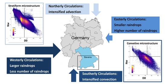
:Quantitative precipitation estimation (QPE) through remote sensing has to take rain microstructure into consideration, because it influences the relationship between radar reflectivity Z and rain intensity R. For this reason, separate equations are used to estimate rain intensity of convective and stratiform rain types. Here, we investigate whether incorporating synoptic scale meteorology could yield further QPE improvements. Depending on large-scale weather types, variability in cloud condensation nuclei and the humidity content may lead to variation in rain microstructure. In a case study for Bavaria, we measured rain microstructure at ten locations with laser-based disdrometers, covering a combined 18,600 h of rain in a period of 36 months. Rain was classified on a temporal scale of one minute into convective and stratiform based on a machine learning model. Large-scale wind direction classes were on a daily scale to represent the synoptic weather types. Significant variations in rain microstructure parameters were evident not only for rain types, but also for wind direction classes. The main contrast was observed between westerly and easterly circulations, with the latter characterized by smaller average size of drops and a higher average concentration. This led to substantial variation in the parameters of the radar rain intensity retrieval equation Z–R. The effect of wind direction on Z–R parameters was more pronounced for stratiform than convective rain types. We conclude that building separate Z–R retrieval equations for regional wind direction classes should improve radar-based QPE, especially for stratiform rain events.
1. Introduction
Understanding rain microstructure can provide us with an insight into the prevailing rain formation processes leading to it. This understanding can be employed in improving quantitative estimation of rain intensity using weather radar, especially in flat regions with high altitude values of the zero degree isotherm [1,2,3,4]. Furthermore, the parametrization of the microphysical processes in numerical weather and climate models can be improved [5,6]. Rain microstructure varies on different spatial scales ranging from few meters [7], to few hundreds of meters [8], to regional [9,10] and global extents [11,12]. This variation also occurs with seasons [13], rain types [14], and large-scale weather types [15,16,17].
A clear example of the different rain formation processes leading to variations in rain drop size distribution is the discrepancy between convective and stratiform rain. This has been quantified in a number of studies [5,14,18,19]. The reason for the difference is the relative importance of cold and warm rain formation processes [20]. Stratiform rain is formed mainly by processes involving ice crystals and interactions of ice with liquid water, while convective rain formation comprises both warm and cold processes. Factors and processes that influence the rain drop size distribution as observed on the ground include rimming and aggregation (above the 0 °C isotherm), condensation (below the 0 °C isotherm), collision, coalescence, turbulence, cloud thickness, electric field, evaporation, and drop fragmentation [21,22]. The difference in rain drop size distribution between convective rain and stratiform rain has been used for the classification of both rain types on the ground. Most of these methods use two rain drop size distribution parameters and a linear discrimination between the regions of rain types [19,23,24,25,26]. Recent methods employed machine learning and reached higher performance levels when using four rain drop size distribution parameters [27,28].
Large-scale weather types denote atmospheric conditions such as the high and low pressure distribution, the position and paths of frontal zones, and the existence of cyclonic or anticyclonic circulation types over a sequence of days [29]. Indirectly, they also influence stream flows [30], floods [31,32,33], debris-flow events [34], forest fires [35,36], air quality, and pollen distribution [37,38,39].
Weather type classification is an important part of statistical climatology [40,41], because these types explain many local weather phenomena. Weather types influence local near-surface temperatures and precipitation [42,43,44,45,46]. They also affect the diurnal cycle of precipitation in terms of frequency and amount [47,48,49], and they impact the occurrence and the magnitude of meteorological extreme events [50,51,52,53,54]. Large-scale weather types may therefore also influence rain microstructure by different rain formation processes being more prevalent under different synoptic scale conditions.
Quantifying rain microstructure under different large-scale weather types may have practical applications for radar-based estimation of rain intensity, because the microstructure influences the relationship between radar reflectivity Z and rain intensity R. For this reason, separate equations are used to estimate rain intensity of convective and stratiform rain type [10,55], instead of using one equation that fits both rain types. A similar improvement of the radar estimation of rain might be possible when considering specific Z–R relations for each of the weather types. We previously reported weather type specific Z–R models with lower errors in estimating rain intensity in Lausanne, Switzerland [17]. Similarly, the influence of weather types on Z–R relationships was also reported for the Cévennes-Vivarais Region, France [16]. However, parameterizing Z–R equations for many weather types definitively requires large amounts of data to represent each class.
Here, we contribute an analysis of the relationship between Z–R parameters and weather types in Central Europe, based on a comprehensive regional dataset of rain microstructure measurements at ten sites in the federal state of Bavaria, Germany. We ask: (1) What is the effect of weather types on rain microstructure, considering both types of rain? and (2) Is there consistent variation in the Z–R parameters between weather types that would suggest opportunities to improve QPE with radar-based methods? To address these questions, we investigate disdrometer records under different large-scale wind direction patterns at a daily scale, and rain type classifications at one-minute intervals over a period of three years.
2. Materials and Methods
2.1. Data Sources and Tools
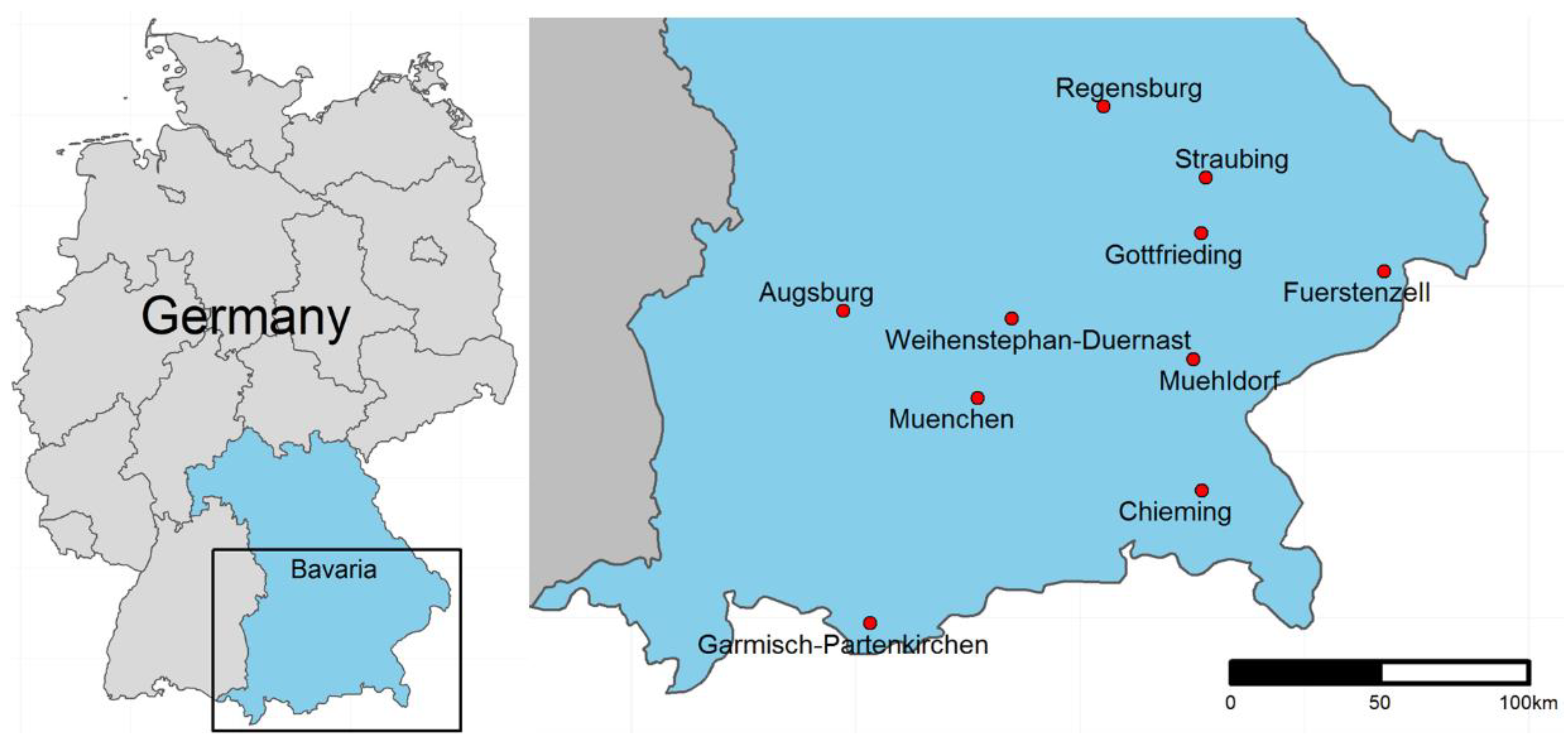
We obtained raw rain drop size distribution measurements from the German Meteorological Service (Deutscher Wetterdienst, DWD), operating a network of Thies disdrometers in Bavaria, in the southeast of Germany (Figure 1). We analyzed measurements at ten sites spanning a period of three years (January 2014–December 2016) with a temporal resolution of one minute. The disdrometers locations cover a distance of 167 km from north to south and 185 km from east to west.
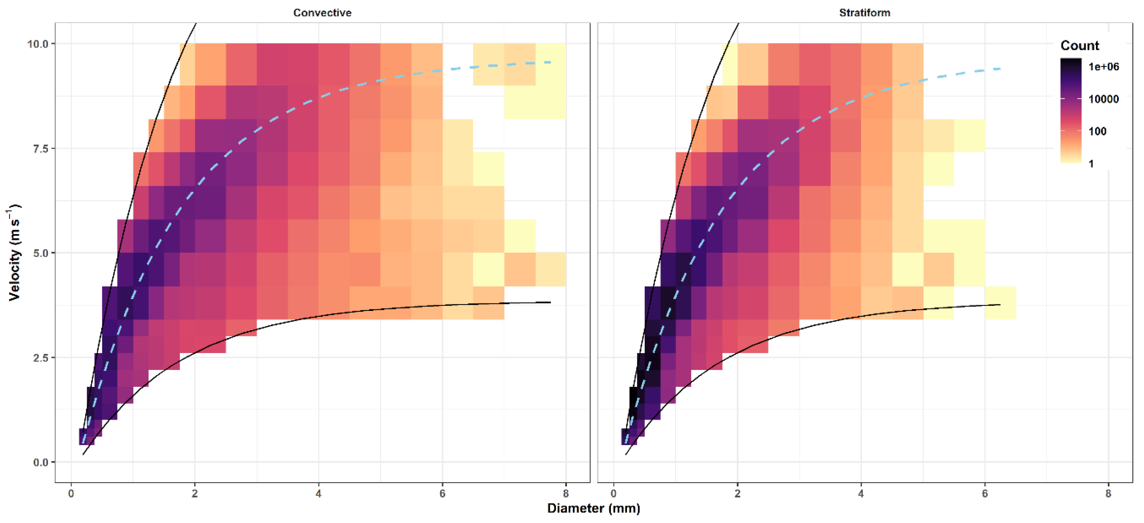
Since raw disdrometer data requires some statistical data cleaning procedures to remove erroneous readings, we followed the filtering procedure of Friedrich et al. [56] and the additional steps of Ghada et al. [17] to remove unrealistically large particles, margin fallers, splashing effects, or readings of insect and spider webs. The filtering procedure removed: (1) All measured particles with a diameter larger than 8 mm; (2) All particles which had a falling velocity less than 60% or greater than 140% of the terminal velocity associated with rain drops of the corresponding diameter [57,58] (Figure 2); (3) Intervals marked by a damaged laser signal or as non-rain intervals by the disdrometer; (4) Intervals which included large drops (D > 5 mm) with low velocities (V < 1 m/h) as an indicator of high wind speed; (5) Intervals with rain intensity lower than 0.1 mm/h [59,60]; (6) Intervals with three or less diameter bins to insure the existence of a drop size distribution. After filtering, the dataset contained a total of 21,705 mm of accumulated rain over a period of 18,633 h.
The DWD classifies large-scale synoptic weather patterns into 40 classes of weather types. The weather type is provided on a daily time scale and is applicable to all of Germany and its surroundings. The classification is based on an operational numerical weather prediction system, i.e., modelling different atmospheric fields such as geopotential height, temperature, relative humidity, and the zonal and meridional components of the wind for several elevations. A detailed explanation of the classification procedure is available online [61], and the full record of weather types is provided by the DWD [62]. Since this classification is performed on daily basis, it would be operationally feasible to associate a separate configuration of the radar rain rate estimate for each weather type class. However, in order to simplify the classification for the purpose of this exploratory case, we grouped all possible classes according to their wind direction index. This index takes one of five possible values: northeasterly (NE), southeasterly (SE), southwesterly (SW), northwesterly (NW), and no prevailing direction (XX). Determining the specific wind direction is based on the number of grid points over Germany with a specific wind direction which needs to exceed 2/3 of the total number of grid points. In case this threshold was not exceeded, the wind direction index is assigned to XX.
2.2. Drop Size Distribution Parameters
Thies disdrometers are laser-based instruments that provide high temporal records of rain microstructure. When a precipitation particle passes between the transmitter and the receiver, the strength of the laser beam is reduced. Based on the magnitude and duration of this reduction, it is possible to estimate the size and velocity of the passing precipitation particle. The Thies disdrometers raw data output represents one-minute summaries of the number of particles in 22 non-linear size classes and 20 non-linear velocity classes. From the raw output, a number of parameters can be obtained. This study is focused particularly on rain intensity R, radar reflectivity Z, total number of drop concentration N, and median volume drop diameter D0.
Rain rate R (mm/h) is given by
where
- : Detected number of drops that fall in diameter range i and velocity range j,
- (s): Temporal resolution (60 s in this case),
- (m2): Corrected detection area:,
- (mm): Mean diameter of drops that fall in diameter range .
The radar reflectivity Z (dBZ) is calculated with the following expression:
where (m/s): Mean velocity of drops that fall in the velocity range .
The total number of drops N (m−3) is computed according to
where (mm): the width of the diameter range .
The rain microstructure is assumed to follow a gamma distribution [72]:
where (mm−1m−3) is the number of drops for each diameter range per unit volume and unite size. The intercept (mm−1−μ m−3), the shape (-), and the slope (mm−1) parameters are determined by the moments method [73]. The nth moment of the raindrop size distribution (mm−1−μ m−3) is given by
and the three gamma parameters are
where
The mass weighted mean diameter Dm (mm), the median volume diameter D0 (mm) and the normalized intercept Nw (mm−1m−3) are calculated based on the parameters of gamma distribution:
Additionally, the classification of rain type into convective and stratiform requires the use of the following parameters: sd_N_10, sd_D0_10, and sd_log10_R_10, where sd_XX_10 is the standard deviation of the values of XX (XX being N, D0 and R, respectively) over a time window of ten minutes.
2.3. Rain Type Classification
Rain type classification was based on an ensemble classifier to predict stratiform versus convective rain based on cloud type, rain intensity, and the standard deviation of rain intensities calculated over the span of ten minutes.
To create a training set for the machine learning model that classifies rain type into convective and stratiform, we obtained records of cloud genera from the DWD [74]. These ground observations were available between July 2013 and August 2014 at Fürstenzell and between July 2013 and January 2014 at Regensburg.
A random forest classification model was trained on the available data from the two locations in this dataset. A combination of two criteria was used for the prior classification, the observation of cloud genus, and the values of R and its standard deviation over five minutes. The model was trained based on the intervals where the prior classification was feasible. It was then used to classify rain in the whole dataset. The spatial variability in rain properties might influence the quality of our classification scheme, especially that the model was trained in only two out of the ten sites. However, the drop in quality on this scale when training in one location and testing in another was minor [28]. More details about the classification procedure are given in Ghada et al [28].
2.4. Retrieving the Parameters of the Z–R Relation
Weather radars usually provide the reflectivity Z which is transformed into rain intensity R using an exponential equation. In our case, R and Z are provided by the disdrometer; therefore, it is possible to get the values of A and b by fitting a linear model to the values of log10(R) and Z.
The radar reflectivity Z is assumed to be related to rain intensity R by the power law:
In this equation, Z is expressed in mm6 m−3. However, Z is usually expressed in the unit decibel relative to Z (dBZ):
By taking the log of Equation (13) and multiplying by 10:
Moreover, based on Equation (14):
a simple linear model is fitted to the values of dBZ and log R which are calculated from the rain drop size distribution. This linear model has the equation:
thus, by comparing Equations (16) and (17) the A and b parameters can be readily found:
Equations (13)–(19) represent the conventional way of retrieving A and b. An alternative method is to consider R as the dependent variable [75]. This method is more appropriate because the main purpose is to reduce errors in estimating R:
By taking the log10 of both sides of Equation (20):
by comparing Equations (22) and (23):
Retrieval of A and b values was done for each event separately. Events with an accumulated rain amount of less than 1 mm were excluded to limit their influence on the fitting process. Additionally, the events were defined by a minimum interevent threshold of 15 min and a minimum duration of 15 min as in Jaffrain and Berne [75]. To ensure clear classification of the rain type on the event level, the fitting was restricted to events during which more than 60% of the event was convective, and events where all intervals were classified as stratiform. The remaining 2449 events contain 9914 h of rain (see Table A1).
3. Results
3.1. Duration and Amount Variation With Rain Type and Wind Direction
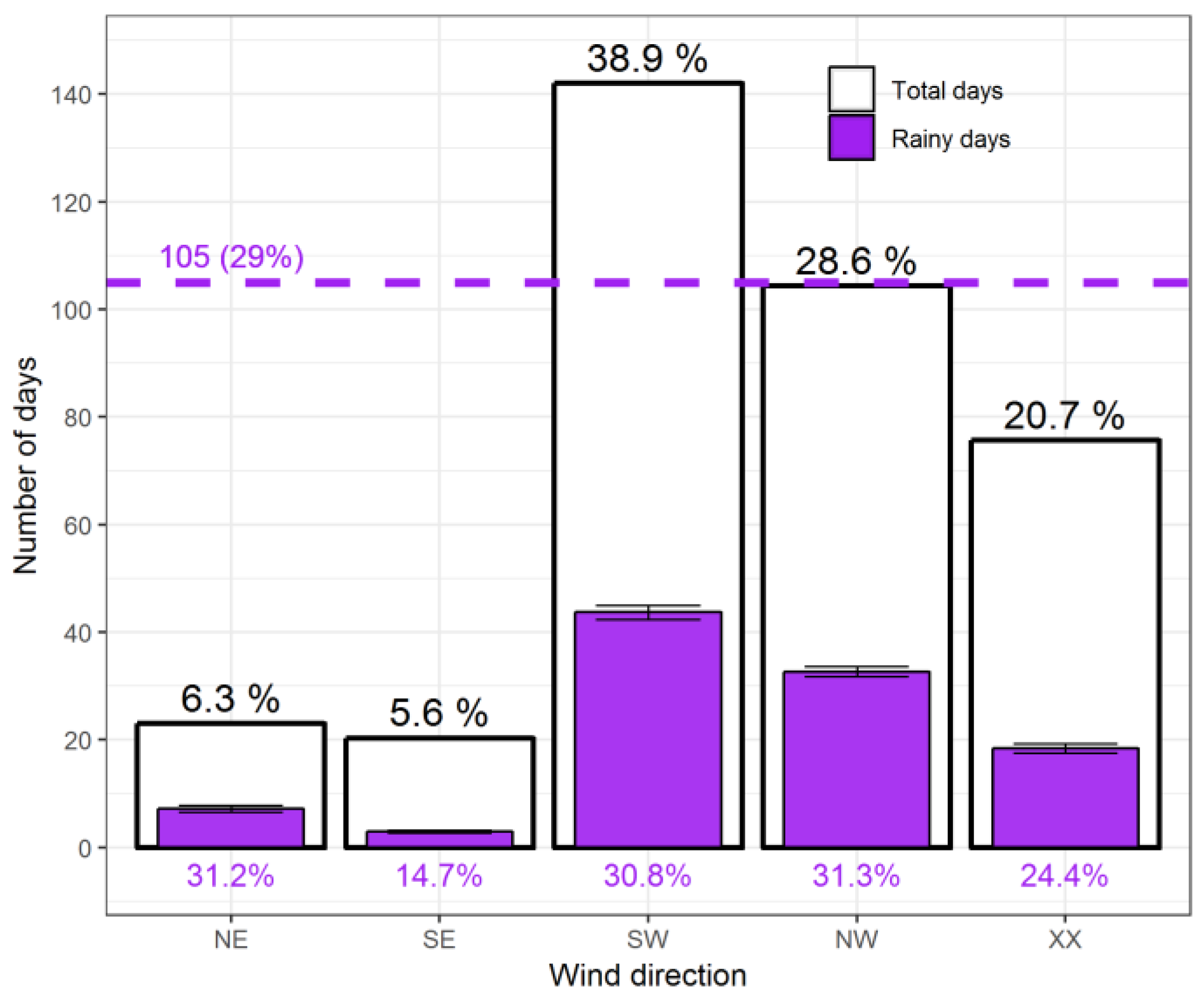
During the 1096 days included in the study period, rain was recorded at least at one station on 515 days. The five wind directions had different frequencies and the most frequent wind directions were the westerly circulations SW and NW with a total of 739 days or two thirds of the time (Figure 3). More than half of these days included rain in at least one station. The easterly circulations accounted for less than 12% of the total number of days. SE had the lowest occurrence and the lowest percentage of rainy days. Both XX and NE had more than 40% rainy days.
When examining the accumulated rain amount and duration, westerly circulations were the dominant wind directions with a contribution reaching 69% of the total rain duration (18,633 h) and total rain amount (21,705 mm) accumulated over all stations (Figure 4). Easterly circulations contributed less than 10% of both rain duration and amount. Convection contributed 36% of the total rain amount and occupied only 8.5% of rain duration. Southerly circulations had the highest proportion of convective rain with around 10% of the total rain duration and more than 40% of the total rain amount, while northerly, and especially northeasterly circulations had a low proportion of convective rain.
The mean stratiform rain intensity was 0.8 mm/h which only marginally varied with wind direction. On the other hand, the mean convective rain intensity of ~5 mm/h considerably varied across wind directions. The highest intensity was associated with SE circulations and the lowest with the NW circulations. Statistical data for each wind direction and rain type including standard deviation (SD) and standard error (SE) are summarized in Table 1.
3.2. Rain Microstructure Variation With Rain Type and Wind Direction
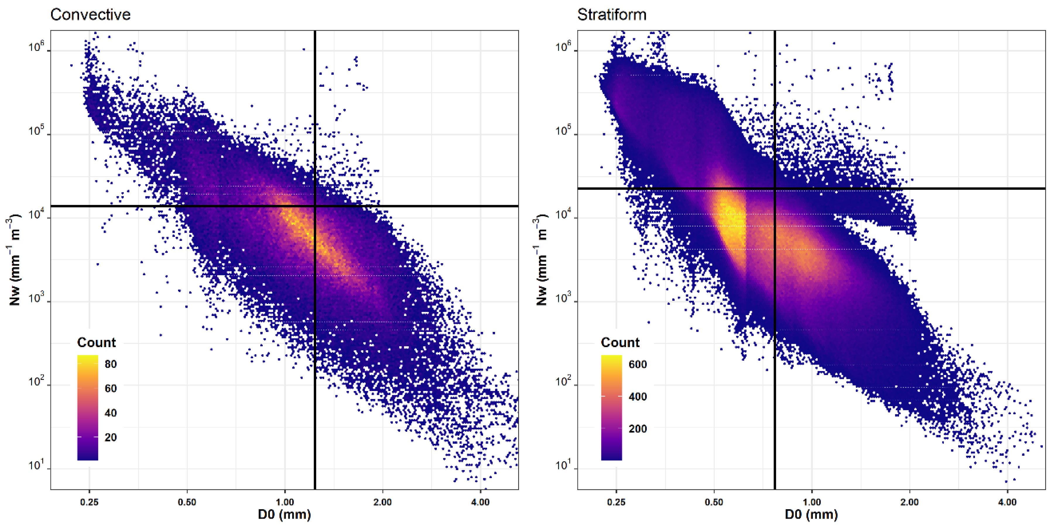
Stratiform rain had smaller drops and lower drop concentrations compared to convective rain (Figure 5). The average D0 for stratiform rain was 0.77 mm compared to 1.24 mm in convective rain. Normalized drop concentration Nw in stratiform rain was around 2.24 × 104 mm−1 m−3, while convective rain had an average of 1.4 × 104 mm−1 m−3. The overall average of D0 (0.81 mm) and Nw (2.17 × 104 mm−1 m−3) were closer to the values of stratiform rain since most rain intervals were of the stratiform type. The clusters in the values of D0 that appear in Figure 5 emerge from the combined effect of the diameter range bins of the disdrometer measurements, and the logarithmic scales on the horizontal axis.
The distributions of D0 and NW values within each wind direction and rain type are illustrated in Figure 6. Similarly, the mean values of D0 and NW for different ranges of rain intensity within each wind direction and rain type are provided in Figure 7.
For stratiform rain, westerly circulations had larger drops and lower drop concentrations compared to easterly circulations. Especially SW had the largest mean D0 and the lowest NW. Easterly circulations were clearly characterized by the smallest drops and the greatest NW. The same pattern was present even when inspecting different classes of rain intensity within stratiform rain (Figure 7). With higher rain intensity, D0 increased too while NW decreased.
For convective rain, only few differences in the previously described patterns were obvious especially when examining the rain microstructure for different ranges of rain intensities. With the exception of SE which had a limited number of convective intervals compared to the remaining wind directions, the median diameter D0 was still the largest in SW and the smallest in NE, while NW was the largest NE and the smallest in Sw. XX and NW had similar NW values but NW exhibited larger drop sizes on average. The wind direction SE did not show any consistent pattern across rain intensity ranges.
When fitting a gamma function to the average rain drop size distribution within each wind direction in stratiform rain (Figure 8), easterly circulations had relatively lower concentrations of drops with a D0 larger than 1 mm compared to westerly circulations. On the other hand, westerly circulations, especially SW, had the lowest concentration of drops with D0 less than 1 mm. In convective rain, northerly circulations exhibited higher proportion of small drops (D0 < 1 mm) and a smaller proportion of large drops compared to southerly circulations. Fitting gamma distribution to rain microstructure was also performed event by event. An example of the fitting for individual events is presented in Figure A1, and the density plots of the gamma distribution parameters are provided in Figure A2.
3.3. Z–R Parameter Variation With Location, Rain Type and Wind Direction
To investigate the influence of rain microstructure variability per wind direction on the rain intensity retrieval equation Z–R, the values of A and b were obtained for 2449 events (see Section 2.4). A density plot of the R and dBZ values for all the 9914 h included in these events is provided in Figure A3. An example of the Z–R equation fitting for one event using two methods is provided in Figure A4.
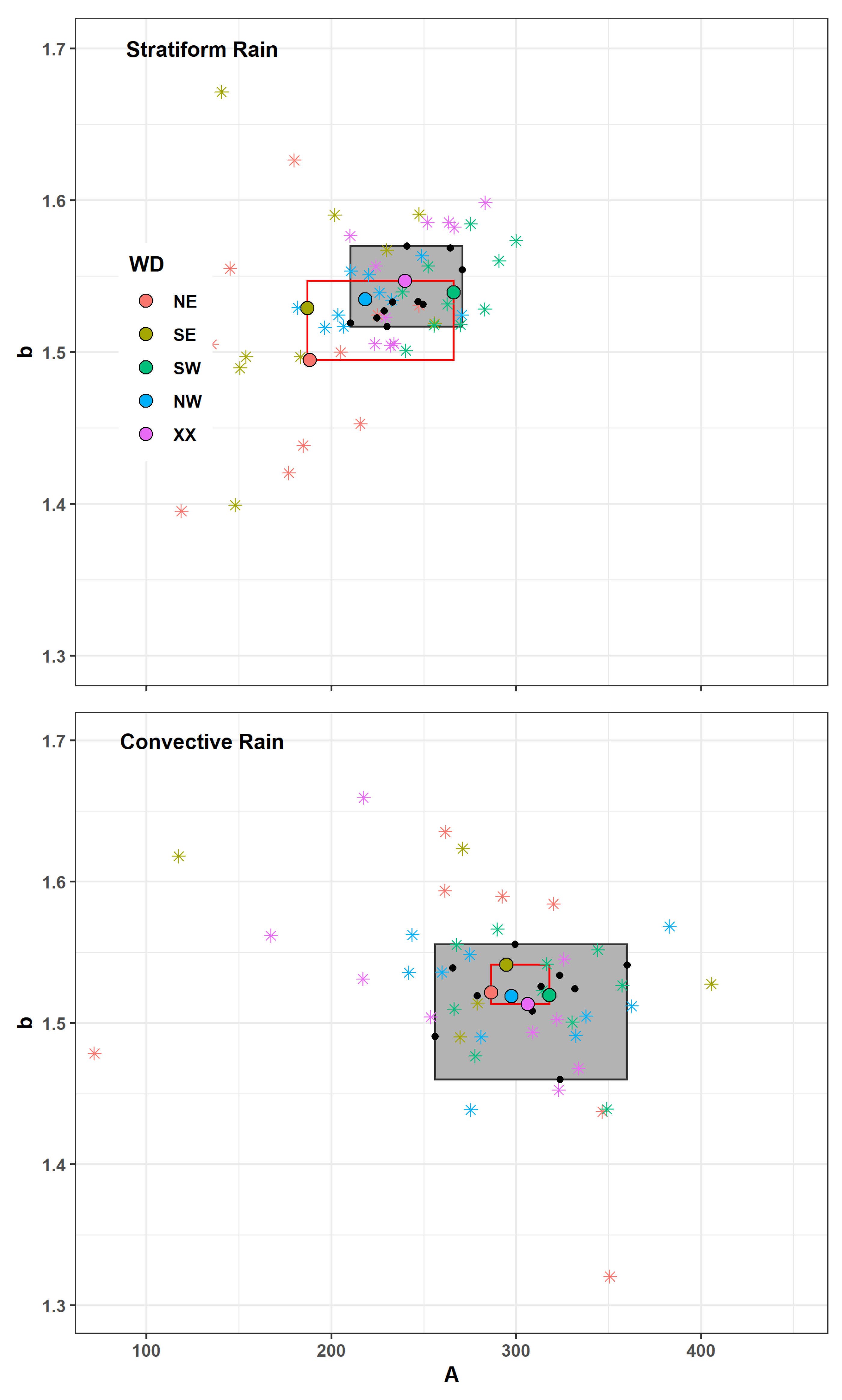
The average value of the prefactor A was clearly larger in convective rain (309) than in stratiform rain (239), while the exponent b value was similar for both rain types (1.53). The values of A and b were averaged for each location (black points in Figure 9; Figure 10), for each wind direction (colored points in Figure 9; Figure 10), and for each combination of location and wind direction (colored stars in Figure 9; Figure 10) in order to demonstrate the variability of A and b with these factors.
In stratiform rain, the range of both mean A and b for each of the ten locations (the grey area in Figure 9) is comparable to the range of the average values for the wind directions (the red rectangle in Figure 9). However, A and b value are smaller in eastern circulation (NE, SE) compared to remaining general wind directions, and they are outside of the range associated with the spatial variability.
In convective rain, no clear pattern was detected for the average values of A and b associated with the five wind directions. The range of A and b values for the different locations is much larger than the range associated with the five general wind directions, indicating a larger spatial variability compared to the variability associated with general wind direction.
When averaging the values of A and b for each combination of location and wind direction, a greater range is observed. In the case of stratiform rain, the pattern of these values is comparable to the one observed for the five general wind directions; SW circulations have larger A values, easterly circulations have smaller A values, while XX and NW circulations fall closely in between. The range of A and b values for each combination of the location and wind direction is larger in the case of convective rain. However, the small number of convective events needs to be considered in this case (see Table A1).
4. Discussion
Our data indicate high frequency and high contribution of westerly and especially SW circulations to the rainy days over Bavaria, Germany. Easterly circulations have the least frequency and especially SE has the lowest share of rainy days. This is in agreement with the frequency of wind directions and proportions of rainy days of long-term studies for Germany for the period between 1995 and 2017 [28]. The high frequency and high contribution of westerly and southwesterly circulations to the number of rainy days is expected for this region since the main moisture flux is westerly [76].
Convection is responsible for 40% of rain amount in this region despite occupying only 10% of rain duration. Similar contributions of convective rain were reported for the Czech Republic [77] and in Switzerland [17]. Convective rain has typically higher rain rates and a distinct microstructure compared to stratiform rain. It is therefore essential to separate convective and stratiform rain prior to addressing rain microstructure, especially considering the variation in convective rain proportion with wind directions [17]. Southerly circulations generally have a higher proportion of convective rain compared to northerly circulations. A possible explanation is the strengthening and inhibition of convection and radiative cooling under different wind directions, which in turn has a major influence on the precipitation diurnal cycle over Germany [49]. Southerly circulations carry along warm air masses which intensify convection in the afternoon and inhibit radiative cooling in the early morning. Northerly circulations, in contrast, transport cold air masses, and therefore suppress convection and intensify radiative cooling.
Westerly circulations need special attention when addressing rain and microstructure, especially with the reported high contribution to rain duration and rain amount, and the expected increase in their frequency over Europe [78,79]. Westerly circulations are associated with larger rain drops than easterly circulations in stratiform rain, while easterly circulations have higher number of drops. This pattern is consistent for both stratiform and convective rain and across the ranges of rain intensity, except for SE circulations in convective rain, which was not well represented by data, accounting only for 0.6% of convective rain amount observed in this study.
Rain microstructure dependence on synoptic weather patterns has previously been reported for other locations in Europe. Northerly circulations in Leon, Spain, were associated with smaller drop sizes, while westerly and southerly circulations had larger rain drops [15]. This pattern was explained by the location of Leon to the south of the Cantabrian Mountains. Northerly circulation air masses precipitate prior to reaching Leon, leaving less humidity, lower rain intensities and smaller drops. Westerly and southerly circulations carry along higher humidity, leading to higher rain intensities and larger drops. For the Cévennes-Vivarais region in France, easterly circulations were associated with lower number of rain drops and larger drop size while most of the westerly circulations had the opposite traits [16]. The associations of rain microstructure with large-scale weather patterns observed in this and other studies are therefore not generally consistent, but region-specific. Different regions have different associated general air-mass characteristics, for example influenced by proximity to the sea or the presence of mountain massifs nearby. The origin of the air masses whether continental or maritime influences the rain microstructure and eventually influences the estimation of precipitation by radars [80,81]. Each class of wind direction used here has a mixture of both maritime and continental origins. It is however assumed that westerly circulations have a larger proportion of air masses with a maritime origin compared to easterly circulations.
The rain microstructure patterns in Bavaria have more in common with the patterns reported for Lausanne, Switzerland. Despite using different disdrometer types, schemes for rain type classification, and weather type classifications, and their different geographical locations in the Alps, easterly circulations were associated with higher number of drops per interval and smaller drop size compared to westerly circulations at both sites [17]. A plausible explanation for this is the variation of humidity and aerosol content in air masses between these wind direction clusters. Aerosols are particularly abundant in air masses which pass over Russia and Eastern Europe, especially over heavy industrialized areas [82,83]. These aerosols act as cloud condensation nuclei [84]. High availability of cloud condensation nuclei increases the number of rain drops in the case of stratiform rain, increases the size of drops in local convection, but has no significant influence on rain microstructure in organized convection [85].
Differences in the load of cloud condensation nuclei under different circulations seem to be a plausible explanation for the rain microstructure differences observed in this study, especially in stratiform rain. The abundance of cloud condensation nuclei in easterly circulations in comparison with westerly circulations leads to higher number of rain drops. This in combination with the high (low) available humidity in westerly (easterly) circulations results in a larger (smaller) size of rain drops, respectively. For convective rain, easterly circulations comprise two wind directions, NE which has the smallest mean D0, and SE which has the largest mean D0. The larger size of raindrops in southerly circulations indicates the intensification of convection when the warm air masses are transported from the south, whereas northerly circulations bring colder airmasses. The rain type classification method used in this study does not differentiate local and organized convection, which makes it impossible to thoroughly compare with the findings of Cecchini et al. [85].
Our results may be useful for radar-based quantitative precipitation estimates (QPE), since Jaffrain et al. [75] demonstrated that the variation of A and b values in the Z–R retrieval equation is an important factor which should be accounted for. In their case study of Lausanne, Switzerland, spatial subgrid variability of rain microstructure was observed, which considerably influenced the quality of the estimation of rain rate. Using the same dataset, Ghada et al. [17] showed that the variability of A and b was larger than the subgrid spatial variability (in an area less than 1 km2) when weather types are considered. In our study, variation of rain microstructure parameters with wind directions in Bavaria led to significant variation in the values of Z–R parameters. The variations in the prefactor A and the exponent b by wind direction are of a similar magnitude as their spatial variations in the case of stratiform rain, but smaller than the spatial variations in the case of convective rain. The same patterns were obtained for the conventional and the alternative methods of Z–R parameters retrieval despite the absolute differences in the values of A and b. These small differences occur because the conventional method is more sensitive to the large values of Z while the alternative method is more sensitive to the density of scatter points where R is below 2.5 mm/h [75]. This difference needs to be addressed in future studies to quantify the exact influence on the estimation of rain intensity by actual radar measurements. Alternatively, the least-rectangles linear regression could be applied as a middle-ground solution.
Assessing potential benefits of considering the variations in Z–R parameters, Jaffrain and Berne [75] concluded that the subgrid spatial variability in rain microstructure may account for errors in rain estimates between −2% and +15%. Variability due to large-scale weather patterns in Z–R parameters is likely to exceed their subgrid spatial variability [17], and based on our study, is comparable with the spatial variability of Z–R parameters in stratiform rain on a regional scale. Consequently, the potential for a significant improvement in rain estimation when accounting for rain microstructure variability by wind direction is expected to be high for radar quantitative precipitation estimates based only on radar reflectivity Z.
However, using only disdrometer data for this purpose would be insufficient because disdrometers provide a direct measurement of rain microstructure, from which R and Z are calculated. These values are accurate local measurements if we assume an accurate measurement of rain microstructure. The next logical research step would be a proper assessment of the improvement potential. This should include the integration of empirical data of radar-based rain intensity estimates validated by ground observations within the different rain types, locations, and large-scale wind directions, as well as a thorough rain type classification based on available instruments, especially considering the available network of dual polarization Doppler radars across Germany. Even for precipitation estimates based on a rain-gauge adjusted system as currently operated by DWD [86], improving the Z–R relation would likely have a positive impact in the final quality of the product.
5. Conclusions
This research demonstrated that rain microstructure varies significantly between weather types in both stratiform and convective rain. Easterly circulations had the highest drop concentration and the smallest drop size while westerly circulations were associated with large drops and low drop concentration. A plausible explanation for these differences is the high humidity content in westerly circulations and abundant cloud condensation nuclei concentration in easterly circulation. These finding offer potential new applications for radar-based quantitative precipitation estimates. Z–R parameters vary substantially with synoptic weather patterns effectively summarized by regional wind direction classes. This variation in Z–R parameters with wind direction approximates their station-to-station spatial variability for stratiform, but not for convective rain. We therefore conclude that building separate Z–R retrieval equation for regional wind direction classes should improve radar-based QPE, especially for stratiform rain events. This approach should be feasible for operational level forecasts, especially since daily large-scale weather types can be predicted with high accuracy several days in advance.
Author Contributions
Conceptualization, W.G. and A.M.; methodology and formal analysis, W.G.; writing—original draft preparation, W.G.; supervision, A.M.; writing—review and editing, W.G., J.B., N.E., A.H. and A.M. All authors have read and agreed to the published version of the manuscript.
Funding
J.B. was partly funded by project RTI2018-098693-B-C32 (AEI/FEDER).
Acknowledgments
We thank the Deutscher Wetterdienst (German Meteorological Service-DWD) for providing the disdrometer data, the classification of weather types, and the cloud observation data. We appreciate the valuable comments provided by the anonymous reviewers. The first author thanks the Deutscher Akademischer Austauschdienst (DAAD) for financial support.
Conflicts of Interest
The funders had no role in the design of the study; in the collection, analyses, or interpretation of data; in the writing of the manuscript, or in the decision to publish the results.
Appendix A

Table A1.
Summary of events selected for the fitting of Gamma distribution and the two methods of R–Z parameters extraction (see Section 2.4).
Table A1.
Summary of events selected for the fitting of Gamma distribution and the two methods of R–Z parameters extraction (see Section 2.4).
| Wind Direction | Rain Type | Duration (h) | # Events | Mean R (mm h−1) | Mean dBZ |
|---|---|---|---|---|---|
| SW | Convective | 144.8 | 236 | 6.1 | 30.7 |
| NW | Convective | 85.7 | 131 | 5.0 | 29.3 |
| XX | Convective | 33.7 | 43 | 6.6 | 30.7 |
| SE | Convective | 11.1 | 10 | 6.5 | 31.6 |
| NE | Convective | 8.6 | 11 | 5.4 | 29.8 |
| SW | Stratiform | 3553.1 | 828 | 0.9 | 20.7 |
| NW | Stratiform | 3063.6 | 618 | 0.9 | 19.6 |
| XX | Stratiform | 2056.0 | 373 | 0.9 | 20.2 |
| NE | Stratiform | 598.8 | 140 | 0.9 | 18.5 |
| SE | Stratiform | 358.8 | 59 | 0.9 | 18.5 |
| Total | 9914.1 | 2449 |
Figure A1.
Raindrop concentration per millimeter and cubic meter for a selection of ten events; one event for each combination of wind direction and rain type. The points represent the event average one-minute concentrations for each diameter range colored by the relevant wind directions. The colored lines represent the fitted gamma distribution for these points.

Figure A2.
The probability density of the fitted gamma parameters in stratiform and convective rain colored by wind directions. The vertical lines represent the mean values of the three parameters based on a selection of 2449 events (see Section 2.4).
Figure A2.
The probability density of the fitted gamma parameters in stratiform and convective rain colored by wind directions. The vertical lines represent the mean values of the three parameters based on a selection of 2449 events (see Section 2.4).

Figure A3.
Density plot of reflectivity (dBZ) and rain intensity (R) for convective and stratiform rain. This plot includes the 9914 h of rain within the selected 2449 events (see Section 2.4).
Figure A3.
Density plot of reflectivity (dBZ) and rain intensity (R) for convective and stratiform rain. This plot includes the 9914 h of rain within the selected 2449 events (see Section 2.4).

Figure A4.
The fitted Z–R lines for one event (start: 2014-09-20 08:48:30, duration: 54 min, rain type: stratiform, wind direction: SW) using both the conventional method (black line) and the alternative method (red line).
Figure A4.
The fitted Z–R lines for one event (start: 2014-09-20 08:48:30, duration: 54 min, rain type: stratiform, wind direction: SW) using both the conventional method (black line) and the alternative method (red line).

References
- Arulraj, M.; Barros, A.P. Improving quantitative precipitation estimates in mountainous regions by modelling low-level seeder-feeder interactions constrained by Global Precipitation Measurement Dual-frequency Precipitation Radar measurements. Remote Sens. Environ. 2019, 231, 111213. [Google Scholar] [CrossRef]
- Steiner, M.; Smith, J.A.; Uijlenhoet, R. A Microphysical Interpretation of Radar Reflectivity–Rain Rate Relationships. J. Atmos. Sci. 2004, 61, 1114–1131. [Google Scholar] [CrossRef]
- Thompson, E.J.; Rutledge, S.A.; Dolan, B.; Thurai, M. Drop Size Distributions and Radar Observations of Convective and Stratiform Rain over the Equatorial Indian and West Pacific Oceans. J. Atmos. Sci. 2015, 72, 4091–4125. [Google Scholar] [CrossRef]
- Ryzhkov, A.V.; Zrnić, D.S. Radar Polarimetry for Weather Observations; Springer: Cham, Switzerland, 2019; ISBN 978-3-030-05092-4. [Google Scholar]
- Steiner, M.; Smith, J.A. Convective versus stratiform rainfall: An ice-microphysical and kinematic conceptual model. Atmos. Res. 1998, 47–48, 317–326. [Google Scholar] [CrossRef]
- Iacobellis, S.F.; McFarquhar, G.M.; Mitchell, D.L.; Somerville, R.C.J. The Sensitivity of Radiative Fluxes to Parameterized Cloud Microphysics. J. Clim. 2003, 16, 2979–2996. [Google Scholar] [CrossRef] [Green Version]
- Jameson, A.R.; Larsen, M.L.; Kostinski, A.B. Disdrometer Network Observations of Finescale Spatial–Temporal Clustering in Rain. J. Atmos. Sci. 2015, 72, 1648–1666. [Google Scholar] [CrossRef] [Green Version]
- Jaffrain, J.; Studzinski, A.; Berne, A. A network of disdrometers to quantify the small-scale variability of the raindrop size distribution. Water Resour. Res. 2011, 47, 2673. [Google Scholar] [CrossRef]
- Doelling, I.G.; Joss, J.; Riedl, J. Systematic variations of Z–R-relationships from drop size distributions measured in northern Germany during seven years. Atmos. Res. 1998, 47–48, 635–649. [Google Scholar] [CrossRef]
- Das, S.; Maitra, A. Characterization of tropical precipitation using drop size distribution and rain rate-radar reflectivity relation. Appl. Clim. 2018, 132, 275–286. [Google Scholar] [CrossRef]
- Gatlin, P.N.; Thurai, M.; Bringi, V.N.; Petersen, W.; Wolff, D.; Tokay, A.; Carey, L.; Wingo, M. Searching for Large Raindrops: A Global Summary of Two-Dimensional Video Disdrometer Observations. J. Appl. Meteor. Clim. 2015, 54, 1069–1089. [Google Scholar] [CrossRef]
- Dolan, B.; Fuchs, B.; Rutledge, S.A.; Barnes, E.A.; Thompson, E.J. Primary Modes of Global Drop Size Distributions. J. Atmos. Sci. 2018, 75, 1453–1476. [Google Scholar] [CrossRef]
- Wen, L.; Zhao, K.; Wang, M.; Zhang, G. Seasonal Variations of Observed Raindrop Size Distribution in East China. Adv. Atmos. Sci. 2019, 36, 346–362. [Google Scholar] [CrossRef]
- Niu, S.; Jia, X.; Sang, J.; Liu, X.; Lu, C.; Liu, Y. Distributions of Raindrop Sizes and Fall Velocities in a Semiarid Plateau Climate: Convective versus Stratiform Rains. J. Appl. Meteor. Clim. 2010, 49, 632–645. [Google Scholar] [CrossRef]
- Fernandez-Raga, M.; Castro, A.; Marcos, E.; Palencia, C.; Fraile, R. Weather types and rainfall microstructure in Leon, Spain. Int. J. Clim. 2017, 37, 1834–1842. [Google Scholar] [CrossRef]
- Hachani, S.; Boudevillain, B.; Delrieu, G.; Bargaoui, Z. Drop Size Distribution Climatology in Cévennes-Vivarais Region, France. Atmosphere 2017, 8, 233. [Google Scholar] [CrossRef] [Green Version]
- Ghada, W.; Buras, A.; Lüpke, M.; Schunk, C.; Menzel, A. Rain Microstructure Parameters Vary with Large-Scale Weather Conditions in Lausanne, Switzerland. Remote Sens. 2018, 10, 811. [Google Scholar] [CrossRef] [Green Version]
- Cerro, C.; Codina, B.; Bech, J.; Lorente, J. Modeling Raindrop Size Distribution and Z (R) Relations in the Western Mediterranean Area. J. Appl. Meteor. 1997, 36, 1470–1479. [Google Scholar] [CrossRef]
- Thurai, M.; Gatlin, P.N.; Bringi, V.N. Separating stratiform and convective rain types based on the drop size distribution characteristics using 2D video disdrometer data. Atmos. Res. 2016, 169, 416–423. [Google Scholar] [CrossRef]
- Munchak, S.J.; Kummerow, C.D.; Elsaesser, G. Relationships between the Raindrop Size Distribution and Properties of the Environment and Clouds Inferred from TRMM. J. Clim. 2012, 25, 2963–2978. [Google Scholar] [CrossRef]
- Rosenfeld, D.; Ulbrich, C.W. Cloud Microphysical Properties, Processes, and Rainfall Estimation Opportunities. Meteorol. Monogr. 2003, 30, 237. [Google Scholar] [CrossRef]
- Villermaux, E.; Bossa, B. Single-drop fragmentation determines size distribution of raindrops. Nat. Phys. 2009, 5, 697–702. [Google Scholar] [CrossRef]
- Tokay, A.; Short, D.A. Evidence from Tropical Raindrop Spectra of the Origin of Rain from Stratiform versus Convective Clouds. J. Appl. Meteor. 1996, 35, 355–371. [Google Scholar] [CrossRef] [Green Version]
- Caracciolo, C.; Prodi, F.; Battaglia, A.; Porcu’, F. Analysis of the moments and parameters of a gamma DSD to infer precipitation properties: A convective stratiform discrimination algorithm. Atmos. Res. 2006, 80, 165–186. [Google Scholar] [CrossRef]
- Caracciolo, C.; Porcù, F.; Prodi, F. Precipitation classification at mid-latitudes in terms of drop size distribution parameters. Adv. Geosci. 2008, 16, 11–17. [Google Scholar] [CrossRef] [Green Version]
- Bringi, V.N.; Williams, C.R.; Thurai, M.; May, P.T. Using Dual-Polarized Radar and Dual-Frequency Profiler for DSD Characterization: A Case Study from Darwin, Australia. J. Atmos. Ocean. Technol. 2009, 26, 2107–2122. [Google Scholar] [CrossRef]
- Bukovčić, P.; Zrnić, D.; Zhang, G. Convective–stratiform separation using video disdrometer observations in central Oklahoma—The Bayesian approach. Atmos. Res. 2015, 155, 176–191. [Google Scholar] [CrossRef]
- Ghada, W.; Estrella, N.; Menzel, A. Machine Learning Approach to Classify Rain Type Based on Thies Disdrometers and Cloud Observations. Atmosphere 2019, 10, 251. [Google Scholar] [CrossRef] [Green Version]
- Baur, F.; Hess, P.; Nagel, H. Kalender der grosswetterlagen Europas 1881–1939. Bad Hombg. 1944, 35. [Google Scholar]
- Steirou, E.; Gerlitz, L.; Apel, H.; Merz, B. Links between large-scale circulation patterns and streamflow in Central Europe: A review. J. Hydrol. 2017, 549, 484–500. [Google Scholar] [CrossRef]
- Petrow, T.; Merz, B.; Lindenschmidt, K.-E.; Thieken, A.H. Aspects of seasonality and flood generating circulation patterns in a mountainous catchment in south-eastern Germany. Hydrol. Earth Syst. Sci. 2007, 11, 1455–1468. [Google Scholar] [CrossRef] [Green Version]
- Nied, M.; Pardowitz, T.; Nissen, K.; Ulbrich, U.; Hundecha, Y.; Merz, B. On the relationship between hydro-meteorological patterns and flood types. J. Hydrol. 2014, 519, 3249–3262. [Google Scholar] [CrossRef] [Green Version]
- Hofstätter, M.; Lexer, A.; Homann, M.; Blöschl, G. Large-scale heavy precipitation over central Europe and the role of atmospheric cyclone track types. Int. J. Clim. 2018, 38, e497–e517. [Google Scholar] [CrossRef] [PubMed] [Green Version]
- Nikolopoulos, E.I.; Borga, M.; Marra, F.; Crema, S.; Marchi, L. Debris flows in the eastern Italian Alps: Seasonality and atmospheric circulation patterns. Nat. Hazards Earth Syst. Sci. 2015, 15, 647–656. [Google Scholar] [CrossRef] [Green Version]
- Kassomenos, P. Synoptic circulation control on wild fire occurrence. Phys. Chem. Earth Parts A B C 2010, 35, 544–552. [Google Scholar] [CrossRef]
- Wastl, C.; Schunk, C.; Lüpke, M.; Cocca, G.; Conedera, M.; Valese, E.; Menzel, A. Large-scale weather types, forest fire danger, and wildfire occurrence in the Alps. Agric. For. Meteorol. 2013, 168, 15–25. [Google Scholar] [CrossRef]
- Russo, A.; Trigo, R.M.; Martins, H.; Mendes, M.T. NO2, PM10 and O3 urban concentrations and its association with circulation weather types in Portugal. Atmos. Environ. 2014, 89, 768–785. [Google Scholar] [CrossRef]
- Nidzgorska-Lencewicz, J.; Czarnecka, M. Winter weather conditions vs. air quality in Tricity, Poland. Appl. Clim. 2015, 119, 611–627. [Google Scholar] [CrossRef] [Green Version]
- Grundström, M.; Dahl, Å.; Ou, T.; Chen, D.; Pleijel, H. The relationship between birch pollen, air pollution and weather types and their effect on antihistamine purchase in two Swedish cities. Aerobiologia 2017, 33, 457–471. [Google Scholar] [CrossRef] [Green Version]
- Ramos, A.M.; Barriopedro, D.; Dutra, E. Circulation weather types as a tool in atmospheric, climate, and environmental research. Front. Environ. Sci. 2015, 3, 44. [Google Scholar] [CrossRef] [Green Version]
- Huth, R.; Beck, C.; Philipp, A.; Demuzere, M.; Ustrnul, Z.; Cahynová, M.; Kyselý, J.; Tveito, O.E. Classifications of atmospheric circulation patterns: Recent advances and applications. Ann. N. Y. Acad. Sci. 2008, 1146, 105–152. [Google Scholar] [CrossRef]
- Buishand, T.A.; Brandsma, T. Comparison of circulation classification schemes for predicting temperature and precipitation in The Netherlands. Int. J. Clim. 1997, 17, 875–889. [Google Scholar] [CrossRef]
- Cortesi, N.; Trigo, R.M.; Gonzalez-Hidalgo, J.C.; Ramos, A.M. Modelling monthly precipitation with circulation weather types for a dense network of stations over Iberia. Hydrol. Earth Syst. Sci. 2013, 17, 665–678. [Google Scholar] [CrossRef] [Green Version]
- Broderick, C.; Fealy, R. An analysis of the synoptic and climatological applicability of circulation type classifications for Ireland. Int. J. Clim. 2015, 35, 481–505. [Google Scholar] [CrossRef] [Green Version]
- Huth, R.; Beck, C.; Kučerová, M. Synoptic-climatological evaluation of the classifications of atmospheric circulation patterns over Europe. Int. J. Clim. 2016, 36, 2710–2726. [Google Scholar] [CrossRef] [Green Version]
- Vallorani, R.; Bartolini, G.; Betti, G.; Crisci, A.; Gozzini, B.; Grifoni, D.; Iannuccilli, M.; Messeri, A.; Messeri, G.; Morabito, M.; et al. Circulation type classifications for temperature and precipitation stratification in Italy. Int. J. Clim. 2018, 38, 915–931. [Google Scholar] [CrossRef]
- Twardosz, R. A synoptic analysis of the diurnal cycle of thunderstorm precipitation in Kraków (Southern Poland). Int. J. Clim. 2009, 26. [Google Scholar] [CrossRef]
- Mandapaka, P.V.; Germann, U.; Panziera, L. Diurnal cycle of precipitation over complex Alpine orography: Inferences from high-resolution radar observations. Q. J. R. Meteorol. Soc. 2013, 139, 1025–1046. [Google Scholar] [CrossRef]
- Ghada, W.; Yuan, Y.; Wastl, C.; Estrella, N.; Menzel, A. Precipitation Diurnal Cycle in Germany Linked to Large-Scale Weather Circulations. Atmosphere 2019, 10, 545. [Google Scholar] [CrossRef] [Green Version]
- Cassano, E.N.; Lynch, A.H.; Cassano, J.J.; Koslow, M.R. Classification of synoptic patterns in the western Arctic associated with extreme events at Barrow, Alaska, USA. Clim. Res. 2006, 30, 83–97. [Google Scholar] [CrossRef] [Green Version]
- Planchon, O.; Quénol, H.; Dupont, N.; Corgne, S. Application of the Hess-Brezowsky classification to the identification of weather patterns causing heavy winter rainfall in Brittany (France). Nat. Hazards Earth Syst. Sci. 2009, 9, 1161–1173. [Google Scholar] [CrossRef] [Green Version]
- Cony, M.; Martin, L. Synoptic patterns that contribute to extremely hot days in Europe. Available online: http://www.scielo.org.mx/scielo.php?script=sci_arttext&pid=S0187-62362010000400001 (accessed on 30 October 2020).
- Nowosad, J.; Stach, A. Relation between extensive extreme precipitation in Poland and atmospheric circulation. Quaest. Geogr. 2014, 33, 115–129. [Google Scholar] [CrossRef] [Green Version]
- Maheras, P.; Tolika, K.; Anagnostopoulou, C.; Makra, L.; Szpirosz, K.; Károssy, C. Relationship between mean and extreme precipitation and circulation types over Hungary. Int. J. Clim. 2018, 38, 4518–4532. [Google Scholar] [CrossRef]
- Kirsch, B.; Clemens, M.; Ament, F. Stratiform and convective radar reflectivity–rain rate relationships and their potential to improve radar rainfall estimates. J. Appl. Meteor. Clim. 2019, 58, 2259–2271. [Google Scholar] [CrossRef]
- Friedrich, K.; Kalina, E.A.; Masters, F.J.; Lopez, C.R. Drop-Size Distributions in Thunderstorms Measured by Optical Disdrometers during VORTEX2. Mon. Wea. Rev. 2013, 141, 1182–1203. [Google Scholar] [CrossRef]
- Atlas, D.; Srivastava, R.C.; Sekhon, R.S. Doppler radar characteristics of precipitation at vertical incidence. Rev. Geophys. 1973, 11, 1. [Google Scholar] [CrossRef]
- Gunn, R.; Kinzer, G.D. The terminal velocity of fall for water droplets in stagnant air. J. Meteorol. 1949, 6, 243–248. [Google Scholar] [CrossRef] [Green Version]
- Chen, B.; Wang, J.; Gong, D. Raindrop Size Distribution in a Midlatitude Continental Squall Line Measured by Thies Optical Disdrometers over East China. J. Appl. Meteor. Clim. 2016, 55, 621–634. [Google Scholar] [CrossRef]
- Angulo-Martínez, M.; Beguería, S.; Latorre, B.; Fernández-Raga, M. Comparison of precipitation measurements by OTT Parsivel 2 and Thies LPM optical disdrometers. Hydrol. Earth Syst. Sci. 2018, 22, 2811–2837. [Google Scholar] [CrossRef] [Green Version]
- Deutscher Wetterdienst. Description of the method and the weather types. Available online: https://www.dwd.de/EN/ourservices/wetterlagenklassifikation/beschreibung.html;jsessionid=5ED0BB104CB32D74A71ADC0C6DE03871.live21064?nn=495490&lsbId=520444 (accessed on 27 September 2019).
- Deutscher Wetterdienst. Weather Type Classification Data. Available online: https://www.dwd.de/EN/ourservices/wetterlagenklassifikation/online_wlkdaten.txt?view=nasPublication&nn=495490 (accessed on 15 October 2019).
- R Core Team. R: A Language and Environment for Statistical Computing; EEA: Vienna, Austria, 2019. [Google Scholar]
- RStudio Team. RStudio: Integrated Development Environment for R.; PBC: Boston, MA, USA, 2018. [Google Scholar]
- Kuhn, M. Caret: Classification and Regression Training. 2018. Available online: https://CRAN.R-project.org/package=caret (accessed on 30 October 2020).
- Meyer, D.; Dimitriadou, E.; Hornik, K.; Weingessel, A.; Leisch, F. E1071: Misc Functions of the Department of Statistics, Probability Theory Group (Formerly: E1071); TU: Wien, Austria, 2018; Available online: https://CRAN.R-project.org/package=e1071 (accessed on 30 October 2020).
- Wickham, H. Reshaping Data with the reshape Package. J. Stat. Softw. 2007, 21, 1–20. [Google Scholar] [CrossRef]
- Robert, J.H. Raster: Geographic Data Analysis and Modeling. 2017. Available online: https://CRAN.R-project.org/package=raster (accessed on 30 October 2020).
- Ryan, M.H. Rmisc: Rmisc: Ryan Miscellaneous. 2013. Available online: https://CRAN.R-project.org/package=Rmisc (accessed on 30 October 2020).
- Hadley, W. Ggplot2. Elegrant Graphics for Data Analysis, 2nd ed.; Springer: Cham, Switzerland, 2016; ISBN 978-3-319-24277-4. [Google Scholar]
- South, A. Rnaturalearth: World Map Data from Natural Earth. 2017. Available online: https://CRAN.R-project.org/package=rnaturalearth (accessed on 30 October 2020).
- Ulbrich, C.W. Natural Variations in the Analytical Form of the Raindrop Size Distribution. J. Clim. Appl. Meteor. 1983, 22, 1764–1775. [Google Scholar] [CrossRef] [Green Version]
- Ulbrich, C.W.; Atlas, D. Rainfall Microphysics and Radar Properties: Analysis Methods for Drop Size Spectra. J. Appl. Meteor. 1998, 37, 912–923. [Google Scholar] [CrossRef]
- Wetterdienst, D. Historical records of hourly cloud type in Germany. Available online: ftp://opendata.dwd.de/climate_environment/CDC/observations_germany/climate/hourly/cloud_type/historical/ (accessed on 16 October 2019).
- Jaffrain, J.; Berne, A. Influence of the Subgrid Variability of the Raindrop Size Distribution on Radar Rainfall Estimators. J. Appl. Meteor. Clim. 2012, 51, 780–785. [Google Scholar] [CrossRef]
- van der Ent, R.J.; Savenije, H.H.G.; Schaefli, B.; Steele-Dunne, S.C. Origin and fate of atmospheric moisture over continents. Water Resour. Res. 2010, 46, 61. [Google Scholar] [CrossRef] [Green Version]
- Rulfová, Z.; Kyselý, J. Trends of Convective and Stratiform Precipitation in the Czech Republic, 1982–2010. Adv. Meteorol. 2014, 2014, 1–11. [Google Scholar] [CrossRef]
- Plavcová, E.; Kyselý, J. Projected evolution of circulation types and their temperatures over Central Europe in climate models. Appl. Clim. 2013, 114, 625–634. [Google Scholar] [CrossRef]
- Stryhal, J.; Huth, R. Trends in winter circulation over the British Isles and central Europe in twenty-first century projections by 25 CMIP5 GCMs. Clim. Dyn. 2019, 52, 1063–1075. [Google Scholar] [CrossRef]
- Das, S.; Chatterjee, C. Rain characterization based on maritime and continental origin at a tropical location. J. Atmos. Sol. Terr. Phys. 2018, 173, 109–118. [Google Scholar] [CrossRef]
- Tenório, R.S.; Cristina da Silva Moraes, M.; Sauvageot, H. Raindrop Size Distribution and Radar Parameters in Coastal Tropical Rain Systems of Northeastern Brazil. J. Appl. Meteor. Clim. 2012, 51, 1960–1970. [Google Scholar] [CrossRef]
- Birmili, W.; Wiedensohler, A.; Heintzenberg, J.; Lehmann, K. Atmospheric particle number size distribution in central Europe: Statistical relations to air masses and meteorology. J. Geophys. Res. 2001, 106, 32005–32018. [Google Scholar] [CrossRef]
- Byčenkienė, S.; Plauškaitė, K.; Dudoitis, V.; Ulevicius, V. Urban background levels of particle number concentration and sources in Vilnius, Lithuania. Atmos. Res. 2014, 143, 279–292. [Google Scholar] [CrossRef]
- Lohmann, U.; Feichter, J. Global indirect aerosol effects: A review. Atmos. Chem. Phys. 2005, 5, 715–737. [Google Scholar] [CrossRef] [Green Version]
- Cecchini, M.A.; Machado, L.A.T.; Artaxo, P. Droplet Size Distributions as a function of rainy system type and Cloud Condensation Nuclei concentrations. Atmos. Res. 2014, 143, 301–312. [Google Scholar] [CrossRef]
- Kreklow, J.; Tetzlaff, B.; Burkhard, B.; Kuhnt, G. Radar-Based Precipitation Climatology in Germany—Developments, Uncertainties and Potentials. Atmosphere 2020, 11, 217. [Google Scholar] [CrossRef] [Green Version]
Figure 1.
Disdrometer locations in Bavaria (SE Germany) that were used to measure rain microstructure, covering a total of 18,600 h of rain in a period of 36 months.
Figure 1.
Disdrometer locations in Bavaria (SE Germany) that were used to measure rain microstructure, covering a total of 18,600 h of rain in a period of 36 months.

Figure 2.
Raindrop count in each diameter-velocity range after the filtering process. The dotted line represents the terminal velocity of each diameter value. The solid lines represent the 60% and the 140% of the terminal velocity.
Figure 2.
Raindrop count in each diameter-velocity range after the filtering process. The dotted line represents the terminal velocity of each diameter value. The solid lines represent the 60% and the 140% of the terminal velocity.

Figure 3.
Frequency of rainy days per year and per wind direction classes that represent large-scale weather types. Rainy days are days on which at least one station recorded five minutes of rain with an intensity of more than 0.2 mm/h. Error bars represent the 95% confidence intervals. Percentages above the white columns represent the overall occurrence of each wind direction and percentages below the columns represent the portion of rainy days in the total number of days within a specific wind direction. The dashed line represents the mean number of rainy days per year.

Figure 4.
Prevalence of convective and stratiform rain types. Accumulated rain duration (a), and rain amount (b) per wind direction averaged over the stations and years. Error bars represent the 95% confidence intervals. The percentages on top of each column represent the proportion of accumulated rain within the respective wind direction to the accumulated rain in the whole year. The percentages below the columns represent the proportion of convective rain to total rain within the respective wind direction.

Figure 5.
Scatter plot of D0 and (NW) for stratiform and convective rain. The vertical and horizontal lines represent the mean values of D0 and NW.
Figure 5.
Scatter plot of D0 and (NW) for stratiform and convective rain. The vertical and horizontal lines represent the mean values of D0 and NW.

Figure 6.
Probability density plots of log10(NW) and D0 for each rain type and wind direction. Vertical thick lines show parameters averaged over all locations for convective (solid red line) and stratiform (dashed thick blue) rain and light lines represent averages for individual locations.
Figure 6.
Probability density plots of log10(NW) and D0 for each rain type and wind direction. Vertical thick lines show parameters averaged over all locations for convective (solid red line) and stratiform (dashed thick blue) rain and light lines represent averages for individual locations.

Figure 7.
Rain microstructure for different rain intensities in stratiform and convective rain. Symbols on each colored line represent summary statistics for a wind direction. Each symbol represents the average median drop size D0 and the normalized drop concentration for a rain intensity range. The intervals were chosen to represent six equal sample sizes and were colored by mean rain intensity. Selected symbols that correspond to equal rain intensity were connected with differently dashed black lines for comparison.

Figure 8.
Raindrop concentration per millimeter diameter and cubic meter for each wind direction in stratiform rain and convective rain. Points represent the one-minute average concentrations for each diameter range colored by wind direction. Colored lines represent the corresponding gamma distribution fits.

Figure 9.
The parameters A and b of the radar rain intensity retrieval equation (Z = ARb) in both rain types using the first method of fitting (Equations (13)–(19)). A and b values are averaged by location (black dots), wind direction (colored circles), and the combination of both (colored stars). The grey area represents the range of A and b for the ten locations. The red rectangle represents the range of A and b for the five general wind directions.

Figure 10.
The parameters of the radar rain intensity retrieval equation (Z = ARb) in both rain types using the second method of fitting (Equations (20)–(25)). A and b values are averaged by location (black dots), wind direction (colored circles), and the combination of both (colored stars). The grey area represents the range of A and b for the ten locations. The red rectangle represents the range of A and b for the five general wind directions.

Table 1.
Summary of rain intensities (R) for wind directions in convective and stratiform rain.
| Rain Type | Wind Direction | Duration (h) | Mean R (mm/h) | Median R (mm/h) | Standard Deviation (mm/h) | Standard Error (mm/h) |
|---|---|---|---|---|---|---|
| Convective | NE | 82.5 | 4.51 | 3.65 | 4.90 | 0.070 |
| SE | 50.7 | 6.23 | 4.83 | 6.41 | 0.116 | |
| SW | 645.6 | 5.11 | 3.72 | 6.09 | 0.031 | |
| NW | 538.1 | 4.33 | 3.36 | 4.89 | 0.027 | |
| XX | 269.6 | 5.80 | 4.54 | 5.79 | 0.046 | |
| Stratiform | NE | 1191.9 | 0.79 | 0.50 | 0.79 | 0.003 |
| SE | 486.2 | 0.80 | 0.46 | 0.92 | 0.005 | |
| SW | 5928.4 | 0.78 | 0.49 | 0.79 | 0.001 | |
| NW | 5740.0 | 0.83 | 0.54 | 0.80 | 0.001 | |
| XX | 3700.8 | 0.84 | 0.52 | 0.89 | 0.002 |
Publisher’s Note: MDPI stays neutral with regard to jurisdictional claims in published maps and institutional affiliations. |
© 2020 by the authors. Licensee MDPI, Basel, Switzerland. This article is an open access article distributed under the terms and conditions of the Creative Commons Attribution (CC BY) license (http://creativecommons.org/licenses/by/4.0/).
Share and Cite
MDPI and ACS Style
Ghada, W.; Bech, J.; Estrella, N.; Hamann, A.; Menzel, A. Weather Types Affect Rain Microstructure: Implications for Estimating Rain Rate. Remote Sens. 2020, 12, 3572. https://doi.org/10.3390/rs12213572
AMA Style
Ghada W, Bech J, Estrella N, Hamann A, Menzel A. Weather Types Affect Rain Microstructure: Implications for Estimating Rain Rate. Remote Sensing. 2020; 12(21):3572. https://doi.org/10.3390/rs12213572
Chicago/Turabian StyleGhada, Wael, Joan Bech, Nicole Estrella, Andreas Hamann, and Annette Menzel. 2020. "Weather Types Affect Rain Microstructure: Implications for Estimating Rain Rate" Remote Sensing 12, no. 21: 3572. https://doi.org/10.3390/rs12213572
Note that from the first issue of 2016, this journal uses article numbers instead of page numbers. See further details here.