Abstract
Imaging Radar Altimeter (IRA) is the current development tendency for ocean surface topography (OST) altimetry, which utilizes Synthetic Aperture Radar (SAR) and interferometry to improve the spatial resolution of OST to several kilometers or even better. Meanwhile, centimetric altimetry accuracy should be guaranteed for applications such as geostrophic currents or marine gravity anomaly inversion. However, the baseline length of IRA which determines the altimetric sensitivity is confined by the satellite platform, in consideration of baseline vibration and payload capability. Therefore, the baseline length from a single satellite can extend to only tens of meters, making it difficult to achieve centimetric accuracy. Referring to the successful experience from TerraSAR-X/TanDEM-X, satellite formation can easily extend the baseline length to hundreds or thousands of meters, depending on the helix orbit. Therefore, we propose the large baseline IRA (LB-IRA) from satellite formation for OST altimetry: the carrier frequency shift (CFS) is brought in to compensate for the severe baseline decorrelation, and the helix orbit is carefully selected to prevent severe time decorrelation from along-track baseline. The numerical results indicate that the LB-IRA, whose cross-track baseline ranges between 629~1000 m and along-tack baseline ranges between 0~40 m, can achieve ~1 cm relative accuracy at 1 km resolution.
1. Introduction
As one of the most fundamental elements in marine dynamic environment, ocean surface topography (OST) is of great significance in climatology, meteorology, and oceanography, such as geostrophic current and marine gravity anomaly inversion [,]. OST is mostly measured by satellite radar altimeter, which sends a special shaped pulse to the nadir and times the round-trip delay to calculate the instantaneous range between ocean surface and the satellite, and after applying several instrumental and geophysical corrections, OST can be precisely extracted []. From the first generation of altimeter on Geosat, to the latest generation on Jason-CS, satellite altimeter has evolved into ~3 cm of altimetric accuracy []. Up to now, all the operational altimetry satellites, such as TOPEX/Poseidon, Jason series, and HY-2A/B, can only measure one-dimensional OST along the orbital track, and the cross-track measurement is realized by combining orbits. Even from satellite constellation, the best achievable grid resolution of interpolated OST is no better than 100~200 km [].
To improve the spatial resolution of OST, the most promising instrument is the so-called Interferometric Synthetic Aperture Radar (InSAR), which records the interferometric phase, instead of timing the round-trip delay for altimetry []. So far, InSAR has been successfully applied in terrain altimetry, however, none of them can be directly used for OST altimetry due to the coarse accuracy, which is no better than a few meters. Therefore, the concept of Imaging Radar Altimeter (IRA) was first proposed by Rodriguez [], which can be considered as the special version of InSAR, dedicated for OST altimetry with an altimetric accuracy that should be at least comparative to traditional radar altimeters []. Another distinguishable characteristic of IRA is its wide swath, which resides along one side of the nadir track and extends to tens of kilometers wide. After aperture synthesis and pulse compression [], the intrinsic resolution of IRA is only a couple of meters.
The most prominent IRA plan is the Surface Water and Ocean Topography (SWOT) mission [,]. The primary payload of SWOT satellite is the Ka-band Radar Interferometer (KaRIn), whose dual transmit/receive antennas are connected by a deployable rigid mast. The interferometric baseline, which is the distance between the phase centers of two antennas, is about 10 m []. The baseline length of KaRIn is much shorter than the 60 m baseline of Shuttle Radar Topography Mission (SRTM), which was dedicated for terrain topography mapping []. To a certain extent, longer baseline results in higher altimetric sensitivity, and furthermore, higher altimetric accuracy. However, SRTM suffers from serious baseline vibration [], which should be strictly constrained by KaRIn as well. To compensate for the insufficient baseline length, the radar look angle of KaRIn is set to be 0.7~4°. SWOT is expected to achieve ~2.5 cm relative accuracy at 1 km resolution (under 1 demand, a swath averaged result among the 50 km swath width []). To fulfill the rigorous accuracy and resolution goal, the SWOT team are facing several technical and engineering problems, and hence the launching date has been postponed several times; recently, SWOT has been scheduled to launch in 2022.
On 15 September 2016, China launched the Tiangong-2 space laboratory, and the Interferometric Imaging Radar Altimeter (InIRA) was one of the experimental payloads on it. The dual Ku-band antennas were mounted outside the capsule, and the baseline length was only 2.3 m, limited by the capsule size. The radar look angle ranges from 1° to 8°, to ensure a swath width of at least 40 km. Based on the acquired data, Kong et al. has evaluated the relative altimetric accuracy of InIRA to be ~3 cm at 10 km resolution []. Though the baseline of InIRA is even shorter than KaRIn, it has proved the great potential in OST altimetry.
Since SWOT KaRIn and Tiangong-2 InIRA both suffer from short baseline deficiency, in reference to the successful practice from TerraSAR-X/TanDEM-X (TSX/TDX) [], we propose the Large Baseline Imaging Radar Altimeter (LB-IRA) from satellite formation, whose baseline length is no longer restrained by a single platform. However, large baseline also aggravates the signal decorrelation, preventing altimetric accuracy from being further improved. We utilize the cross-interferometry method, of which a small carrier frequency shift (CFS) is introduced in between two transmitted signals to compensate for the severe baseline decorrelation. The principle of cross-interferometry was first proposed by Gatelli [], and further verified by ERS-ENVISAT terrain datasets [,,,]. As for LB-IRA, a helix orbit is carefully selected to prevent severe time decorrelation from along-track baseline while maintaining a minimum safety distance. Furthermore, in order to prevent radio interference while maintaining a sufficient swath width, the idea of matching CFS with signal bandwidth is introduced for the first time, innovated by the principle of frequency division multiplexing. The numerical results indicate that the LB-IRA system can achieve ~1 cm relative accuracy on a 1 km resolution grid.
The paper is organized as follows: Section 2 briefly introduces the IRA altimetry principle and defines the concept of relative/absolute altimetric accuracy, and Section 3 discusses the helix orbit configuration in consideration of arranging proper cross-track/along-track baseline. The principle of cross-interferometry, and the design principle of several key parameters in consideration of CFS, is discussed in Section 4, and the methodology for system parameter selection and phase noise suppression are explained in Section 5. Section 6 presents and analyzes the numerical results of the altimetric accuracy based on the system parameters of LB-IRA, and the last section (Section 7) summarizes the whole paper.
2. Measurement Principle
2.1. Altimetry Principle
The altimetry principle of IRA is basically triangulation, inherited from InSAR. As shown in Figure 1, two antennas measure the ranges to the target at slightly different geometry due to the existence of baseline, , the range difference, , related to the target height is recorded by the interferometric phase []. Based on triangulation, the height of the target is expressed as:
where is the altitude of antenna phase center on Sat1, is the range between the target and the phase center, and is the radar look angle from Sat1 to the target.
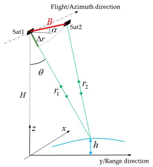
Figure 1.
Schematic diagram of triangulation altimetry of Imaging Radar Altimeter (IRA).
Altitude, H, and range, , can be precisely measured by other means, only leaving the look angle, , which varies with the target height unknown. However, the interferometric phase is directly related to the look angle as:
where is the so-called interferometric phase, i.e., the phase difference between two complex images of IRA, B is the baseline length, is the baseline inclination angle, and is the radar wavelength determined by center carrier frequency.
Based on Equations (1) and (2), the target height can be expressed as []:
the approximation on the right side of the equation is true when . The baseline length of IRA is no larger than a few kilometers, which meets the approximation condition. The approximated equation can be used to derive altimetric error transfer functions for simplification, however, only the non-approximation equation should be used to calculate the target height, since any approximation may introduce major altimetric errors.
The altimetric accuracy is determined by all kinds of errors, the most significant ones are baseline length error, baseline inclination error, and interferometric phase error. Based on Equation (3), the altimetric error transfer functions are derived from partial differentiation:
where is the target position along the range direction.
Equation (4) indicates that the altimetric error introduced by baseline length error, , is affected by the baseline length, baseline inclination, altitude, and radar look angle. The selection of altitude and baseline inclination has limited degrees of freedom; therefore, small look angle and large baseline should be set to reduce the altimetric error.
Equation (5) indicates that small look angle decreases the altimetric error induced by baseline inclination error, , and the altimetric error increases linearly with target position along the range direction. Different from single-platform IRA, whose baseline is usually formed by rigid mast, the baseline of LB-IRA is quite flexible, therefore the baseline inclination error is mostly from baseline length error instead of attitude jitter of the platform [], as shown in Figure 2.
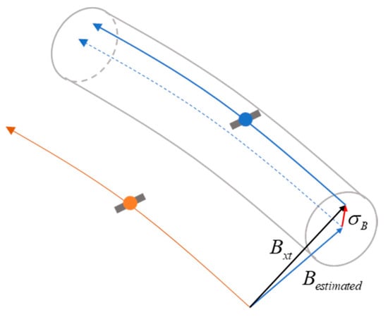
Figure 2.
Baseline inclination error of Large Baseline Imaging Radar Altimeter (LB-IRA) introduced by baseline length error.
According to Figure 2, the baseline inclination error between two satellites can be expressed as []:
where is the cross-track baseline length, and is the baseline length estimated from the orbit track. Apparently, for LB-IRA, large baseline can relatively decrease the altimetric error.
Equation (6) indicates that large baseline or small look angle leads to low altimetric error introduced by interferometric phase error. Interferometric error includes phase bias and random phase noise: the phase bias part can usually be calibrated, and therefore, the phase noise ultimately determines the altimetric accuracy level [].
From the above analysis, we have noticed that large baseline can improve the altimetric accuracy. However, large baseline can also deteriorate the phase noise level, and thus prevent further improving altimetric accuracy from increasing the cross-track baseline length. The contradiction can be solved by cross-interferometry, which will be addressed later in Section 4.
2.2. Relative Altimetric Accuracy
For marine applications such as geostrophic current inversion or gravity anomaly inversion, the relative altimetric accuracy is being more concerned than absolute accuracy, since the physical variables are inversed from the OST gradient instead of the absolute value. Apart from phase noise, all parameter errors of IRA will introduce spatial correlated altimetric error along the range direction, as indicted by variable in Equations (4)–(6). Figure 3 gives the example of altimetric error introduced by baseline inclination error. The error increases linearly along the range direction, the absolute altimetric error is defined as the difference between True OST and OST measured from IRA, and the relative altimetric error is defined as the difference between two adjacent points, A and B.
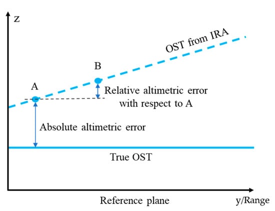
Figure 3.
Schematic diagram of relative and absolute altimetric error.
The relative altimetric error related to baseline length error, baseline inclination error, and phase noise, are as follows:
where is the horizontal distance between two points; in this paper, it stands for the grid resolution after multi-looking. Comparing Equations (8)–(10) to Equations (4)–(6), it appears that the relative altimetric errors are usually much smaller than the absolute errors since most of the common part has been cancelled out by differentiation. Therefore, the relative altimetric accuracy of IRA is determined by systematic parameter errors and the final resolution of the OST product.
3. Satellite Formation and Interferometry Baseline
3.1. Helix Orbit Configuration
The main objective of LB-IRA from satellite formation is to extend the baseline length, which is essential for improving altimetric accuracy. Different from single-platform interferometry, the baseline formed by satellite formation is flexible without any mast, thus the baseline length is determined by the orbit configuration. In order to obtain a cross-track baseline, a tiny angle is introduced between two orbit planes, as shown in Figure 4a. To provide passive safety in case of a vanishing along-track separation, the suggested safety formation distance should be larger than 150 m, hence a small eccentricity is introduced which yields the radial separation at the poles, as shown in Figure 4b. This type of orbit configuration is referred to as helix orbit by the TSX/TDX team [].
Figure 4.
LB-IRA satellite formation and the helix orbit configuration. (a) Maximum separation at equator, intersects near the poles, (b) maximum separation at equator, the small eccentricity offset causes different heights of perigee, snd (c) optional rotation of the perigee to achieve proper baseline configuration near the high-latitude region.
Under the helix orbit configuration, the variation cycle of cross-track/along-track baseline length could be adjusted by thrusters at the initial stage, and the cross-track baseline reaches its maximum length while the along-track baseline is about zero at the equator; after that, along-track baseline length starts to increase, and reaches its maximum near the poles. Since ocean surface is randomly changing, OST altimetry near the high latitude region will suffer from worse time decorrelation due to larger along-track separation. Therefore, the optional rotation of the argument of perigee can be adjusted to achieve proper baseline configuration [], as shown in Figure 4c; however, at the same time, the low-latitude region will no longer be suitable for OST altimetry.
3.2. Along-Track Baseline and Time Decorrelation
Different from single-platform interferometry, the triangulation of satellite formation is formed by two different time-space planes (except when the satellite formation is at the equator), as shown in Figure 5. At moment, Sat1 is ahead of Sat2, right in the triangulation area (the gray shaded area); after , Sat2 reaches to the same area, therefore the along-track baseline of LB-IRA is inevitable during OST altimetry.
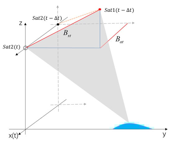
Figure 5.
Interferometry by LB-IRA.
The orbital velocity of ocean surface wave will aggravate the time decorrelation considerably, eventually decreasing the altimetric accuracy. The echoes received by two antennas of LB-IRA are from a combination of multiple wavelike scatterers within the same specific region, however with different time moments due to the along-track separation. Because of the randomness of wave orbital velocity of the scatterers, the doppler spectrum of two received echoes statistically deviate from each other []. The ocean coherence time can be used to quantify the statistics of doppler spectrum of ocean surface wave, and higher sea state (usually determined by surface wind velocity) and radar waveband lead to shorter ocean coherence time. The time decorrelation can then be expressed as []:
where is the ocean coherence time, is the time-lag determined by the along-track baseline, and is the satellite velocity. In consideration of other technical and engineering issues, the waveband of LB-IRA is chosen to be Ku-band (center carrier frequency is about 13.5~13.6 GHz). The surface wind velocity is set to be 7.4 m/s ( result) based on one year of statistical data from Cross-Calibrated Multi-Platform []. According to the evaluation method from Reference [], assuming surface wave propagates along the orbit track, the ocean coherence time is about 8 milliseconds at the Ku-band and under 7.4 m/s of wind velocity. According to Equation (11), the interferometric coherence will decrease to 0.79 due to time decorrelation, which corresponds to about 40 m of the along-track separation at the altitude of 891 km. Since IRA interferometric data will suffer from all kinds of decorrelations, we decided that 0.8 should be the lower bound for time decorrelation.
3.3. Baseline Variation Cycle
Under the helix orbit configuration, in consideration of the along-track baseline limitation, the angle between orbit plane, satellite altitude, and orbit inclination is set to be 7.88 m °, 891 km, and 78°, respectively. The orbit center deviates ~53 m from the earth center, to maintain a minimum safety distance of 150 m during the orbital cycle, as shown in Figure 6a. The variation cycle of cross-track and along-track baseline length are shown in Figure 6b,c, respectively. The cross-track baseline length reaches its maximum at the equator and decreases as latitude increases. The along-track baseline length reaches its minimum at the equator and increases as latitude increases, and the positive/negative sign stands for the relative position change of two satellites. In order to avoid severe time decorrelation, the suggested interferometry region should be within 44.6° northern/southern latitude, where the along-track baseline length is shorter than 40 m, and the across-track baseline length ranges between 629~1000 m, as indicated by the blue shaded area in Figure 6b,c. The baseline inclination angle is small and poses a minor influence to OST altimetry within the 44.6° latitude range.
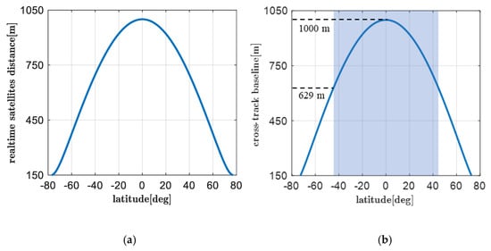
Figure 6.
Real-time distance and baseline variation versus latitude during half an orbit cycle. (a) Real-time distance, (b) cross-track baseline length, (c) along-track baseline length, and (d) baseline inclination angle.
According to Figure 6c, under the helix orbit configuration, OST altimetry near the high-altitude region will suffer from severe time decorrelation. In order to improve the altimetric accuracy, the orbit perigee can be adjusted for proper baseline length near the latitude region of interest.
4. CFS for Baseline Decorrelation Compensation
The cross-track baseline length of LB-IRA ranges between 629~1000 m, which is far larger than that of SWOT. Though SWOT has chosen the Ka-band and near-nadir look angle for short baseline defection, its altimetric sensitivity is still much lower than that of LB-IRA. However, too-large baseline also decreases the signal coherence due to baseline decorrelation, preventing altimetric accuracy from further being improved. In this section, we introduce the carrier frequency shift (CFS) method for baseline decorrelation compensation, hence LB-IRA will work in cross-interferometry mode to achieve much higher altimetric accuracy than normal interferometry.
4.1. Principle of Baseline Decorrelation
The interferometry of microwave also follows the optical diffraction grating principle from physical optics, therefore, the essential reason for baseline decorrelation is the radar look angle difference, which introduces a relative shift between the target spectrum received by two antennas [,]. The dual antennas in normal interferometry mode transmit pulses of the same carrier frequency and bandwidth, or, in other words, the transmitted spectrum window for target observing is identical, as shown in the upper left corner of Figure 7. The transmitted pulse eventually measures the target in space domain, and the spatial frequency of the target is usually defined as wavenumber, i.e., the reciprocal of the wavelength. Due to the tiny difference of look angle, the transmitted spectrum window will be shifted and stretched after being projected to the wavenumber domain (the stretching effect can be omitted since radar carrier frequency is much higher than signal bandwidth), as shown in the bottom of Figure 7. Only the overlapped region of wavenumber can be used for interferometry, leaving the non-overlapped part to decay to phase noise.
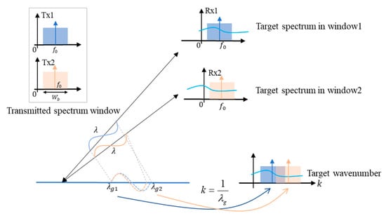
Figure 7.
Schematic diagram of the principle of baseline decorrelation.
Since wavenumber and frequency are basically the same physical quantity in space and time domain, therefore, the wavenumber shift can be equally expressed by frequency shift []:
where is the radar carrier frequency, is the vertical component of cross-track baseline, and is the average slope of ocean surface which changes the local incidence angle of microwave. According to Equation (12), longer vertical baseline and smaller look angle result in a bigger non-overlapped part of the received target spectrum, and since the envelope of the target spectrum is relatively flat, the baseline decorrelation can be expressed as []:
From Equation (13), we learn that enlarging the bandwidth can relatively restrain baseline decorrelation. However, a larger bandwidth leads to lower signal-to-noise ratio (SNR), as well as heavier data transmitting volume, which should be avoided to facilitate extensive OST altimetry. Besides, the cross-track baseline of LB-IRA can extend to 1000 m or even longer and enlarging the signal bandwidth cannot be of much help since the frequency shift is far larger than the signal bandwidth. Figure 8 shows the frequency shift versus radar look angle: the cross-track baseline length is 1000 m in this case. The frequency shift can reach to 180~760 MHz among the angle range of 0.7~4°, which is far bigger than the bandwidth of most of the spaceborne SAR/InSAR. It appears that larger look angle can alleviate the demand for wider bandwidth, however, even if the look angle increases to 20°, the maximum coherence is only 0.69, affected by baseline decorrelation alone, under the 100 MHz of bandwidth setting.
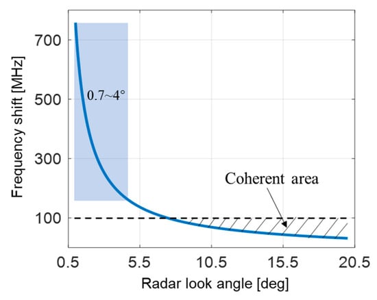
Figure 8.
Frequency shift versus radar look angle.
4.2. Design Princile of CFS
According to the principle of baseline decorrelation, a carrier frequency shift (CFS) can be introduced in between two transmitted signals, in order to shift back the non-overlapped part of the received spectrum as much as possible, and eventually compensate for the severe baseline decorrelation []. The CFS method in this paper is also named as cross-interferometry, first verified by the ERS-ENVISAT dataset, however, the dataset cannot be used to verify OST altimetry since the minimum interferometry time-lag is 28 min, during which the signals are no longer correlated due to time decorrelation.
The along-track baseline length of LB-IRA is 40 m at most in case of severe time decorrelation, however, the dual antennas both send pulses for interferometry, and therefore, the received signals may suffer from radio interference with each other. In order to prevent radio interference, the CFS and bandwidth should be compatible with each other. As shown in Figure 9, the CFS is set to be based on Equation (12) to compensate for the baseline decorrelation. The bandwidth of the transmitted pulses is , the bandwidth should be smaller than the CFS, so that the transmitted spectrum windows will not overlap with each other, as shown in the upper left corner of Figure 9. The received signal spectrum of both antennas are exactly the same, after being demodulated with the carrier frequency of and , respectively. Therefore, only the corresponding part of the spectrum can be demodulated correctly as a baseband signal. After bandpass filtering, the signal spectrum overlaps with each other very well owing to CFS, besides, the radio interference is avoided since the band-pass filter is designed according to the signal bandwidth.
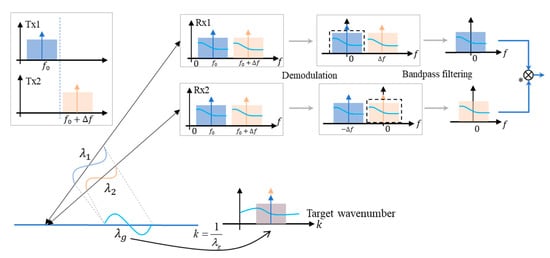
Figure 9.
Proper design of carrier frequency shift (CFS) and signal bandwidth to avoid radio interference. The * along with the circle with a multiplication sign in it, stands for complex multiplication, which is a standard operation for SAR signal processing.
Cross-interferometry or CFS compensation is easy to implement since the carrier frequency and bandwidth are programmable by Field-Programmable Gate Array (FPGA) nowadays []. The critical part is how to properly design the CFS to achieve both centimetric accuracy and kilometer resolution. According to Equation (12), the CFS is determined by several key parameters of LB-IRA, most of which are correlated or mutually restricted with each other. Therefore, the optimal design principle of CFS should be addressed for LB-IRA. The following focuses on the design principle of CFS, in terms of radar look angle, ocean surface slope, and the cross-track baseline length.
4.2.1. Radar Look Angle
During the selection of CFS, the swath width of LB-IRA and SNR should be taken into consideration while choosing the proper radar look angle. The look angle varies within a certain range to acquire a swath width of 50 km, at least. According to Figure 8, a smaller center look angle leads to wider variation range of look angle in order to cover up the swath width, and eventually, larger CFS variation range since the frequency shift is determined by radar look angle.
However, the CFS method can only select a constant frequency shift for the entire swath. The selected CFS may perfectly compensate for the baseline decorrelation at the swath center, however, it leaves the other part of the swath only partially compensated. Figure 10 shows the spectrum overlap before and after CFS; around the center range where CFS is selected accordingly, the spectrum perfectly overlaps with each other after CFS. However, due to the variation of radar look angle, the spectrum only partially overlaps with each other around the near or far range of the swath.
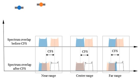
Figure 10.
Spectrum overlap before and after CFS along the range direction.
Figure 11a,b shows the coherence before and after CFS compensation, the cross-track baseline length and bandwidth are set to be 1000 m and 40 MHz, respectively. The look angle ranges of 9~12° and 12~15° cover up nearly the same swath width of 50 km, however the CFS variation of 9~12° is larger than that of 12~15°. Before CFS compensation, as shown in Figure 11a, the coherence is zero from the swath center to the near swath since the spectrum has no overlap part due to a smaller look angle. Only a small part of the spectrum overlaps with each other near the far range as the radar look angle increases, due to limited signal bandwidth. After CFS compensation, as shown in Figure 11b, although both of the coherence are high at the swath center (corresponds to center look angle), the coherence of 9~12° decreases more sharply than 12~15° due to larger CFS variation, as indicated by the dashed line in Figure 11a. Apparently, 12~15° is more preferable since the coherence is higher and more consistent among the entire swath.
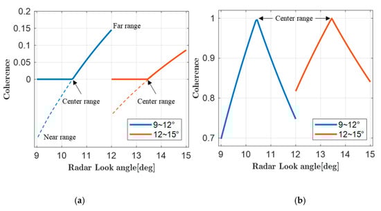
Figure 11.
Coherence determined by baseline decorrelation, (a) before CFS compensation, and (b) after CFS compensation.
However, too-large look angle may decrease the SNR significantly since the normalized radar cross-section (NRCS) decreases as radar look angle increases, and the decorrelation by thermal noise will get worse. Referring to the NRCS from Global Precipitation Mission (GPM) [], 12~15° of radar look angle is selected for LB-IRA, which compensates for the baseline decorrelation well among the entire swath and maintains a reasonable SNR level as well.
4.2.2. Cross-Track Baseline Length
Although the decorrelation from large baseline can be well-compensated by CFS, larger baseline also leads to smaller altimetric ambiguity, and further leads to more severe volume decorrelation. The volume decorrelation of ocean surface is different from terrain [], introduced by the random distribution of surface wave height as well as the slightly different measurement geometry. As shown in Figure 12, the received echoes by LB-IRA antennas are from a combination of multiple scatterers within the same resolution grid. LB-IRA records an echo as a complex number, the phase of which is directly related to satellite-ocean surface range, and because of the randomness of surface wave height, the range-associated phase recorded by two antennas deviate from each other, as indicated in Figure 12 by blue and yellow arrows within the complex plane, the summation of which suffer from a certain degree of randomness, or equally speaking, the signal decorrelation.
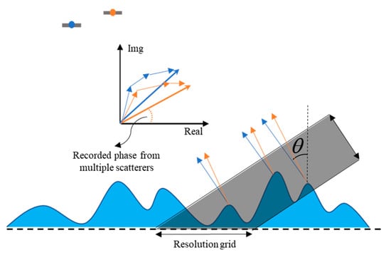
Figure 12.
Schematic diagram of wave volume decorrelation.
To quantify the wave volume decorrelation, suppose surface wave height follows the Gaussian distribution, then, the coherence decided by wave volume decorrelation can be expressed as []:
where is the standard deviation of interferometric phase, and is the standard deviation of surface wave height of ocean surface, related to the significant wave height (SWH) as . Figure 13a,b shows the wave volume decorrelation under different SWH settings, where the cross-track baseline length of each is 629 and 1000 m, respectively. The SWH = 2 m situation corresponds to of global ocean wave height distribution. From Figure 13, we learn that though CFS can compensate for the baseline decorrelation, the wave volume decorrelation still gets worse as the baseline length increases. In order to avoid severe wave volume decorrelation, the cross-track baseline length is restricted below 1000 m for the LB-IRA.
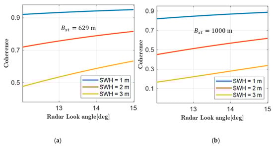
Figure 13.
Coherence determined by wave volume decorrelation. (a) Cross-track baseline length of 629 m, and (b) cross-track baseline length of 1000 m.
4.2.3. Ocean Surface Slope
The slope here refers to the ocean surface slope that extends beyond at least one resolution grid of 1 km. The influence of the wave slope variation within one resolution grid causes the signal decorrelation rather than frequency shift and can be decomposed into wave volume or time decorrelation, etc.
The OST variation is normally less than a few decimeters over a spatial extension of tens or hundreds of kilometers. Suppose a sub-mesoscale eddy of 50 km diameter and 50 cm height anomaly located in the middle of the swath, then the slope introduced by the eddy is merely arcsec, and its influence to frequency shift can be totally omitted. Under rough condition where surges may reside, the slope could be large enough that it causes a non-negligible frequency shift, however, the OST altimetry of LB-IRA is restricted to work below level 4 of sea state (corresponds to SWH smaller than 2 m), since OST of high sea state is considered unreliable.
5. Methodology for Altimetric Accuracy Analysis
5.1. Parameters Setting
The altimetric errors of LB-IRA are mainly introduced from interferometric phase noise, baseline inclination, and length error. The interferometric phase noise is determined by the signal coherence, therefore, LB-IRA works in cross-interferometry mode which introduces the CFS to compensate for baseline decorrelation. Apart from baseline decorrelation, time decorrelation, thermal decorrelation, and wave volume decorrelation should all be taken into consideration while selecting the system parameters. The signal coherence can also be improved by averaging neighboring resolution cells, usually referred to as multi-looking by the InSAR community, which will be explained later.
The altimetric error from baseline inclination or length error can only be decreased by longer cross-track, higher radar band, or smaller radar look angle. Therefore, apart from the CFS method, proper system parameters must be selected for LB-IRA. Figure 14 shows the flowchart of the methodology for parameters selection. Since the LB-IRA is mainly focused on geostrophic current or marine gravity anomaly inversion, whether the systems parameters are properly selected is determined if the centimetric relative accuracy is achieved at 1 km resolution.
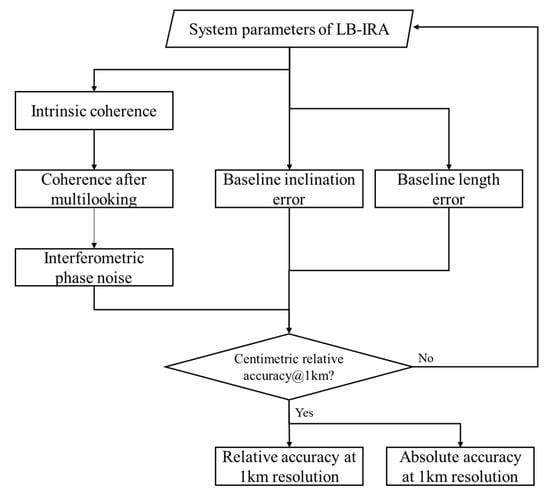
Figure 14.
Flowchart of the methodology for parameters selection.
The main system parameters for numerical analysis are listed in Table 1. Since the baseline length that determines the CFS varies with latitude, the CFS needs to be accommodated with varying latitude during the orbit cycle, besides, the bandwidth needs to be accommodated with varying CFS in case of radio interference. Therefore, the CFS and its corresponding radar carrier frequency and bandwidth vary within a recommended range rather than being a fixed value, as listed in Table 1.

Table 1.
System parameters.
5.2. Multi-Looking
The total coherence which ultimately determines the phase noise level of LB-IRA can be expressed as:
where is the baseline decorrelation in cross-interferometry mode, is the thermal decorrelation, is the wave volume decorrelation, and is the time decorrelation. In addition to the above decorrelation factors, quantization, ambiguities, and processing, etc., all may lead to signal decorrelation, however, they can be considered minor comparing to those major ones. The total coherence is shown in Figure 15, along with all major decorrelation factors as well, and the parameters used for numerical analysis are from Table 1. Figure 15a,b corresponds to the results of 629 and 1000 m of cross-track baseline length, respectively. The total coherence of 629 m is above 0.5, and as the cross-track baseline length increases to 1000 m, the total coherence decreases due to more severe wave volume decorrelation, however, it is still above 0.4 throughout most of the swath.
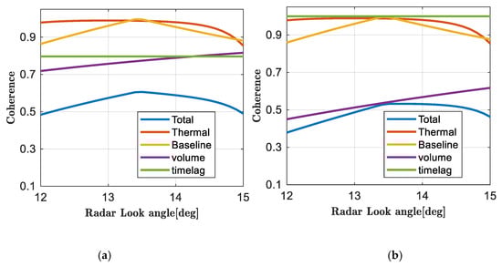
Figure 15.
Total coherence alongside other major decorrelation factors of LB-IRA. (a) Cross-track baseline length of 629 m, and (b) cross-track baseline length of 1000 m.
The phase noise due to coherence loss can be considered as white noise, hence spatial averaging, or, in other words, multi-looking, can be utilized to suppress phase noise in order to increase the altimetric accuracy [,]. Different from terrain topography, OST varies extremely mildly, therefore, large numbers of independent pixels of intrinsic resolution can be multi-looked. The phase noise standard deviation after multi-looking is []:
where is the total coherence before multi-looking, , are the number of independent resolution cells along the range and azimuth direction respectively, and are the intrinsic resolution along range and azimuth direction respectively, and is the grid resolution after multi-looking.
6. Numerical Results of LB-IRA
The altimetric accuracy of LB-IRA is evaluated and discussed based on the selected parameters from Table 1. Figure 16a, b shows the absolute altimetric accuracy determined by phase noise alone, under a cross-track baseline length of 629 and 1000 m, respectively. Although the total coherence of LB-IRA is relatively low, as shown in Figure 15, owing to multi-looking, which considerably suppresses the phase noise, the absolute altimetric accuracy still meets the centimetric accuracy requirement at 1 km resolution. Assuming the phase noise of two neighboring grids are totally uncorrelated, then, the relative accuracy will be decreased by a factor of , which is still better than 1 cm for most cases.
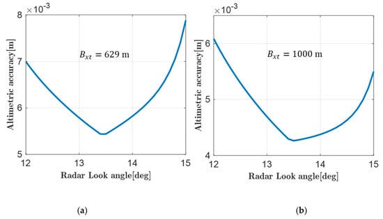
Figure 16.
The absolute altimetric accuracy determined by phase noise, at 1 km resolution. (a) Cross-track baseline length of 629 m, and (b) cross-track baseline length of 1000 m.
According to Reference [], the baseline length error of TSX/TDX is smaller than 1 mm by DGPS evaluation. Figure 17a shows the absolute accuracy determined by a baseline length error of 1 mm, the absolute accuracy is a few centimeters among the variation range of cross-track baseline. The relative accuracy determined by the same baseline length error is shown in Figure 17b. Due to differentiation which cancels out most of the common parts of error, the relative accuracy is far better than the centimetric requirement.
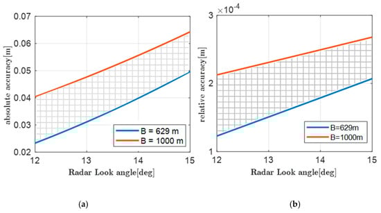
Figure 17.
The altimetric accuracy determined by a baseline length error of 1 mm. (a) The absolute accuracy and (b) the relative accuracy.
According to Equation (7), a baseline length error of 1 mm will result in an equivalent inclination error of 0.2~0.3 arcsec, corresponding to the baseline length of 629~1000 m. Figure 18a indicates that the absolute centimetric accuracy cannot be met without further calibration from the ground, which is also the same dilemma faced by SWOT []. However, the relative accuracy is as high as 1~2 mm, as shown in Figure 18b, which is quite sufficient for applications such as geostrophic current or marine gravity anomaly inversion.
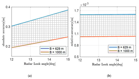
Figure 18.
The altimetric error determined by an equivalent baseline inclination error. (a) The absolute accuracy and (b) the relative accuracy.
Although the relative altimetric accuracy of LB-IRA can be as high as a few millimeters, the absolute accuracy still cannot fulfill the centimetric accuracy requirement at present. The biggest altimetric error comes from the baseline length error, due to limited ranging accuracy between two satellites. If the ranging accuracy can be improved by an order of magnitude by calibration from the ground, or utilizing other advanced ranging techniques, for example, the K-band ranging system on Gravity Recovery And Climate Experiment (GRACE) satellite whose accuracy is only a couple of microns [], the altimetric capability of LB-IRA will be improved remarkably.
7. Conclusions
This paper proposed the LB-IRA from satellite formation which utilizes CFS to compensate for large baseline decorrelation. The simulation results indicate that ~1 cm relative accuracy can be achieved at 1 km resolution. The LB-IRA is currently a possible solution rather than a specific satellite mission for OST altimetry. Comparing to single satellite altimetry, the advantages of satellite formation are:
- The CFS method can release the baseline length limitation from baseline decorrelation, also increasing the freedom of selecting other interferometric parameters.
- The altimetric error associated to phase noise is only a few millimeters, which is quite extraordinary owing to much larger baseline length than that of the single platform.
- It poses relatively easier or fewer technical or engineering challenges, such as the rigorous attitude control accuracy, or the mast vibration or dilation error that should be addressed by the SWOT team.
- The relative altimetric accuracy is quite consistent throughout the entire swath, facilitating marine application based on the OST gradient.
However, one major issue to be addressed is the limited observation coverage of LB-IRA; due to time decorrelation, the suggested altimetry region is within 44.6° N/S latitude at an orbit inclination of 78°. The possible solution is to adjust the orbit perigee so that the along-track baseline is short at the high-latitude region, as shown in Figure 4c. An alternative solution for the insufficient coverage is to launch two sets of LB-IRAs, however, this is at the cost of a higher budget.
Another issue is the restricted condition for conducting OST altimetry. The SWH should be smaller than 2 m for higher reliability of the altimetry result, which is the same dilemma faced by any other IRA as well. However, since one of the primary applications for LB-IRA is ocean bathymetry inversion (which requires centimetric relative accuracy of OST at least), a large volume of data within a long time range may compensate for the limited observation efficiency.
Author Contributions
Conceptualization, W.K. and B.L.; funding acquisition, B.L.; investigation, W.K. and B.L.; methodology, W.K.; supervision, B.L. and J.S.; writing—original draft, W.K.; writing—review and editing, W.K., B.L., J.S., R.Z. and X.S. All authors have read and agreed to the published version of the manuscript.
Funding
This research was funded by Qian Xuesen Lab.—DFH Sat. Co Joint Research and Development Fund (Grant No. M-2017-006), the National Defense Science and Technology Innovation Special Zone Project (Grant No. Y-SYS-GZZ-SK-002), and the National Natural Science Foundation of China (Grant No. 42074225).
Acknowledgments
We would like to thank the support from the “National defense Basic research program” and the “China Aerospace Science and Technology Corporation Limited independent research and development project”.
Conflicts of Interest
The authors declare no conflict of interest.
References
- Fu, L.-L.; Chelton, D.B.; Le Traon, P.-Y.; Morrow, R. Eddy dynamics from satellite altimetry. Oceanography 2010, 23, 14–25. [Google Scholar] [CrossRef]
- Sandwell, D.T.; Smith, W.H. Marine gravity anomaly from Geosat and ERS 1 satellite altimetry. J. Geophys. Res. Solid Earth 1997, 102, 10039–10054. [Google Scholar] [CrossRef]
- Chelton, D.B.; Ries, J.C.; Haines, B.J.; Fu, L.-L.; Callahan, P.S. Satellite altimetry. In International Geophysics; Elsevier: Amsterdam, The Netherlands, 2001; Volume 69, pp. 1–2. [Google Scholar]
- Scharroo, R.; Bonekamp, H.; Ponsard, C.; Parisot, F.; von Engeln, A.; Tahtadjiev, M.; de Vriendt, K.; Montagner, F. Jason continuity of services: Continuing the Jason altimeter data records as Copernicus Sentinel-6. Ocean Sci. 2016, 12, 471–479. [Google Scholar] [CrossRef]
- Quartly, G.D.; Legeais, J.-F.; Ablain, M.; Zawadzki, L.; Fernandes, M.J.; Rudenko, S.; Carrère, L.; García, P.N.; Cipollini, P.; Andersen, O.B. A new phase in the production of quality-controlled sea level data. Earth Syst. Sci. Data 2017, 9, 557–572. [Google Scholar] [CrossRef]
- Bamler, R.; Hartl, P. Synthetic aperture radar interferometry. Inverse Probl. 1998, 14, R1. [Google Scholar] [CrossRef]
- Rodriguez, E.; Pollard, B.; Martin, J. Wide-swath ocean altimetry using radar interferometry. IEEE Trans. Geosci. Remote Sens. 1999. Available online: http://hdl.handle.net/2014/17962 (accessed on 23 September 2020).
- Fu, L.-L.; Ubelmann, C. On the transition from profile altimeter to swath altimeter for observing global ocean surface topography. J. Atmos. Ocean. Technol. 2014, 31, 560–568. [Google Scholar] [CrossRef]
- Moreira, A.; Prats-Iraola, P.; Younis, M.; Krieger, G.; Hajnsek, I.; Papathanassiou, K.P. A tutorial on synthetic aperture radar. IEEE Geosci. Remote Sens. Mag. 2013, 1, 6–43. [Google Scholar] [CrossRef]
- Fu, L.-L.; Alsdorf, D.; Morrow, R.; Rodriguez, E.; Mognard, N. SWOT: The Surface Water and Ocean Topography Mission: Wide-Swath Altimetric Elevation on Earth; Jet Propulsion Laboratory, National Aeronautics and Space: Pasadena, CA, USA, 2012.
- Fu, L.-L.; Alsdorf, D.; Rodriguez, E.; Morrow, R.; Mognard, N.; Lambin, J.; Vaze, P.; Lafon, T. The SWOT (Surface Water and Ocean Topography) mission: Spaceborne radar interferometry for oceanographic and hydrological applications. In Proceedings of the OCEANOBS’09, Venice, Italy, 21–25 September 2009. [Google Scholar]
- Agnes, G.S.; Waldman, J.; Peterson, L.; Hughes, R. Testing the Deployment Repeatability of a Precision Deployable Boom Prototype for the Proposed SWOT KaRIn Instrument. In Proceedings of the 2nd AIAA Spacecraft Structures Conference, Kissimmee, FL, USA, 5–9 January 2015; p. 1838. [Google Scholar]
- Farr, T.G.; Rosen, P.A.; Caro, E.; Crippen, R.; Duren, R.; Hensley, S.; Kobrick, M.; Paller, M.; Rodriguez, E.; Roth, L. The shuttle radar topography mission. Rev. Geophys. 2007, 45. [Google Scholar] [CrossRef]
- Van Zyl, J.J. The Shuttle Radar Topography Mission (SRTM): A breakthrough in remote sensing of topography. Acta Astronaut. 2001, 48, 559–565. [Google Scholar] [CrossRef]
- Fjørtoft, R.; Gaudin, J.-M.; Pourthié, N.; Lalaurie, J.-C.; Mallet, A.; Nouvel, J.-F.; Martinot-Lagarde, J.; Oriot, H.; Borderies, P.; Ruiz, C. KaRIn on SWOT: Characteristics of near-nadir Ka-band interferometric SAR imagery. IEEE Trans. Geosci. Remote Sens. 2013, 52, 2172–2185. [Google Scholar] [CrossRef]
- Kong, W.; Chong, J.; Tan, H. Performance analysis of ocean surface topography altimetry by Ku-Band Near-Nadir interferometric SAR. Remote Sens. 2017, 9, 933. [Google Scholar] [CrossRef]
- Moreira, A.; Krieger, G.; Hajnsek, I.; Hounam, D.; Werner, M.; Riegger, S.; Settelmeyer, E. TanDEM-X: A TerraSAR-X add-on satellite for single-pass SAR interferometry. In Proceedings of the IGARSS 2004. 2004 IEEE International Geoscience and Remote Sensing Symposium, Anchorage, AK, USA, 20–24 September 2004; pp. 1000–1003. [Google Scholar]
- Gatelli, F.; Guamieri, A.M.; Parizzi, F.; Pasquali, P.; Prati, C.; Rocca, F. The wavenumber shift in SAR interferometry. IEEE Trans. Geosci. Remote Sens. 1994, 32, 855–865. [Google Scholar] [CrossRef]
- Wegmüller, U.; Santoro, M.; Werner, C.; Strozzi, T.; Wiesmann, A.; Lengert, W. DEM generation using ERS–ENVISAT interferometry. J. Appl. Geophys. 2009, 69, 51–58. [Google Scholar] [CrossRef]
- Arnaud, A.; Adam, N.; Hanssen, R.; Inglada, J.; Duro, J.; Closa, J.; Eineder, M. ASAR ERS interferometric phase continuity. In Proceedings of the IGARSS 2003. 2003 IEEE International Geoscience and Remote Sensing Symposium. Proceedings (IEEE Cat. No. 03CH37477), Toulouse, France, 21–25 July 2003; pp. 1133–1135. [Google Scholar]
- Perissin, D.; Prati, C.; Engdahl, M.E.; Desnos, Y.-L. Validating the SAR wavenumber shift principle with the ERS–Envisat PS coherent combination. IEEE Trans. Geosci. Remote Sens. 2006, 44, 2343–2351. [Google Scholar] [CrossRef]
- Santoro, M.; Askne, J.I.; Wegmuller, U.; Werner, C.L. Observations, modeling, and applications of ERS-ENVISAT coherence over land surfaces. IEEE Trans. Geosci. Remote Sens. 2007, 45, 2600–2611. [Google Scholar] [CrossRef]
- Rodriguez, E.; Martin, J. Theory and design of interferometric synthetic aperture radars. In Proceedings of the IEE Proceedings F (Radar and Signal Processing); April 1992; pp. 147–159. Available online: https://digital-library.theiet.org/content/journals/10.1049/ip-f-2.1992.0018 (accessed on 26 October 2020).
- Krieger, G.; Moreira, A.; Fiedler, H.; Hajnsek, I.; Werner, M.; Younis, M.; Zink, M. TanDEM-X: A satellite formation for high-resolution SAR interferometry. IEEE Trans. Geosci. Remote Sens. 2007, 45, 3317–3341. [Google Scholar] [CrossRef]
- Esteban-Fernandez, D. SWOT Project Mission Performance and Error Budget Document. JPL D-79084; 2014; pp. 41–43. Available online: https://pdms.jpl.nasa.gov/ (accessed on 23 September 2020).
- Reale, F.; Pugliese Carratelli, E.; Di Leo, A.; Dentale, F. Wave orbital velocity effects on radar Doppler altimeter for sea monitoring. J. Mar. Sci. Eng. 2020, 8, 447. [Google Scholar] [CrossRef]
- Suchandt, S.; Romeiser, R. X-band sea surface coherence time inferred from bistatic SAR interferometry. IEEE Trans. Geosci. Remote Sens. 2017, 55, 3941–3948. [Google Scholar] [CrossRef]
- Frasier, S.J.; Camps, A.J. Dual-beam interferometry for ocean surface current vector mapping. IEEE Trans. Geosci. Remote Sens. 2001, 39, 401–414. [Google Scholar] [CrossRef]
- Prati, C.; Rocca, F. Improving slant-range resolution with multiple SAR surveys. IEEE Trans. Aerosp. Electron. Syst. 1993, 29, 135–143. [Google Scholar] [CrossRef]
- Chua, M.Y.; Koo, V.C. FPGA-based chirp generator for high resolution UAV SAR. Prog. Electromagn. Res. 2009, 99, 71–88. [Google Scholar] [CrossRef]
- Nouguier, F.; Mouche, A.; Rascle, N.; Chapron, B.; Vandemark, D. Analysis of dual-frequency ocean backscatter measurements at Ku-and Ka-bands using near-nadir incidence GPM radar data. IEEE Geosci. Remote Sens. Lett. 2016, 13, 1310–1314. [Google Scholar] [CrossRef]
- Alberga, V. Volume decorrelation effects in polarimetric SAR interferometry. IEEE Trans. Geosci. Remote Sens. 2004, 42, 2467–2478. [Google Scholar] [CrossRef]
- Peral, E.; Rodríguez, E.; Esteban-Fernández, D. Impact of surface waves on SWOT’s projected ocean accuracy. Remote Sens. 2015, 7, 14509–14529. [Google Scholar] [CrossRef]
- Dibarboure, G.; Labroue, S.; Ablain, M.; Fjortoft, R.; Mallet, A.; Lambin, J.; Souyris, J.-C. Empirical cross-calibration of coherent SWOT errors using external references and the altimetry constellation. IEEE Trans. Geosci. Remote Sens. 2011, 50, 2325–2344. [Google Scholar] [CrossRef]
- Kim, J.; Lee, S.W. Flight performance analysis of GRACE K-band ranging instrument with simulation data. Acta Astronaut. 2009, 65, 1571–1581. [Google Scholar] [CrossRef]
Publisher’s Note: MDPI stays neutral with regard to jurisdictional claims in published maps and institutional affiliations. |
© 2020 by the authors. Licensee MDPI, Basel, Switzerland. This article is an open access article distributed under the terms and conditions of the Creative Commons Attribution (CC BY) license (http://creativecommons.org/licenses/by/4.0/).