What Can We Learn from the CloudSat Radiometric Mode Observations of Snowfall over the Ice-Free Ocean?


1
DIATI, Politecnico di Torino, 10129 Turin, Italy
2
Earth Observation Science Group, Department of Physics and Astronomy, University of Leicester, Leicester LE1 7RH, UK
3
National Centre for Earth Observation, University of Leicester, Leicester LE1 7RH, UK
4
National Research Council of Italy (CNR), Institute of Atmospheric Sciences and Climate (ISAC), 00133 Rome, Italy
*
Author to whom correspondence should be addressed.
Remote Sens. 2020, 12(20), 3285; https://doi.org/10.3390/rs12203285
Submission received: 5 September 2020
/
Revised: 3 October 2020
/
Accepted: 6 October 2020
/
Published: 10 October 2020
(This article belongs to the Special Issue Radar Remote Sensing of Cloud and Precipitation)
Abstract
:The quantification of global snowfall by the current observing system remains challenging, with the CloudSat 94 GHz Cloud Profiling Radar (CPR) providing the current state-of-the-art snow climatology, especially at high latitudes. This work explores the potential of the novel Level-2 CloudSat 94 GHz Brightness Temperature Product (2B-TB94), developed in recent years by processing the noise floor data contained in the 1B-CPR product; the focus of the study is on the characterization of snow systems over the ice-free ocean, which has well constrained emissivity and backscattering properties. When used in combination with the path integrated attenuation (PIA), the radiometric mode can provide crucial information on the presence/amount of supercooled layers and on the contribution of the ice to the total attenuation. Radiative transfer simulations show that the location of the supercooled layers and the snow density are important factors affecting the warming caused by supercooled emission and the cooling induced by ice scattering. Over the ice-free ocean, the inclusion of the 2B-TB94 observations to the standard CPR observables (reflectivity profile and PIA) is recommended, should more sophisticated attenuation corrections be implemented in the snow CloudSat product to mitigate its well-known underestimation at large snowfall rates. Similar approaches will also be applicable to the upcoming EarthCARE mission. The findings of this paper are relevant for the design of future missions targeting precipitation in the polar regions.
1. Introduction
Snowfall is an important physical element of the Earth’s water and energy cycles, and its continuous monitoring and quantification on a global scale is fundamental to globally quantify water resources, and for understanding feedback mechanisms and interconnections in hydrology and climate. High latitude regions, where observations and measurements are sparse and the processes poorly known, are experiencing significant changes brought about by climate change, but the impact on precipitation, as well as on snow/ice extent and properties, and related feedback mechanisms, is not well documented and understood.
Remote sensing of snowfall remains among the most challenging tasks in global precipitation retrieval ([1,2,3,4,5,6,7], and many others). As opposed to visible-infrared (VIS-IR; N.B.: a full list of acronyms is provided in the Appendix A) sensors, used to analyse upper-level cloud structure and convective cloud properties, spaceborne microwave sensors have been largely used to extract quantitative information on snowfall, thanks to their ability to penetrate clouds. Passive microwave (PMW) sensors have high frequency channels (90–190 GHz) that are highly sensitive to the snowflakes scattering (e.g., [8,9]), and thanks to their large swath and availability on many platforms they ensure good global coverage and lengthy data records. However, the detection and quantification of snowfall by passive microwave observations is challenging because it involves complex and dynamic interactions between the cloud liquid and ice hydrometeors, atmospheric conditions, and the surface ([1,10,11].
Spaceborne radars, although not specifically designed to comprehensively characterize global snowfall, offer a valuable source of consistent measurements to observe falling snow. Cloud-oriented missions, such as CloudSat [12] (and EarthCARE [13] in the near future), offer high sensitivity thanks to their W-band (94 GHz) cloud profiling radar (CPR) that enables observing the vertical distribution of hydrometeors and to retrieve surface snowfall [14,15,16,17,18,19]. Several studies have demonstrated that CloudSat CPR sensitivity (−28 to −30 dBZ) and orbital characteristics (sampling from 82° N–82° S latitudes) allow it to be employed successfully for global snowfall research (e.g., [14,20,21]. A complete overview of CloudSat CPR capabilities to address fundamental snowfall monitoring questions on a global, seasonal and regional basis is provided by [19]. CloudSat has provided unprecedented data sets for the study of clouds and global snowfall up to 82° of latitude (e.g., [3,22,23,24]), including unique snowfall modes (e.g., cumuliform snow, [25]), that were previously unavailable from observational means on a near-global scale. In a recent paper by [26], an extensive validation of surface snowfall rate estimates from GPM products and from the CloudSat CPR shows that CPR snowfall rate estimates are by far in better agreement with the ground-based radar estimates than any other algorithm.
However, some CPR limitations need to be mentioned. CPR limited swath (with a revisiting time of 16 days for a square of 100 × 100 km2) does not provide the needed coverage for snowfall global monitoring. At W band, reflectivities for snow tend to saturate near 20 dBZ because of reduced backscattering efficiency of larger aggregates relative to lower frequencies and compensating effects of hydrometeor attenuation and multiple scattering in heavier, deeper snow events (e.g., [27]). These weaknesses are partly compensated by the Ku/Ka-band scanning Dual-frequency Precipitation Radar (DPR) on board the Global Precipitation Measurement (GPM) mission Core Observatory [11], but DPR lower sensitivity (and limited latitudinal coverage) does not allow to properly account for light snowfall occurrence and quantification in global snowfall climatology [6,28].
It is important to mention other CloudSat CPR limitations for snowfall observations. First, CPR reflectivity observations are contaminated by ground clutter, typically in the 1000 m closest to the surface [17,23,29,30]. Since retrieving surface snowfall rate requires extrapolating the values from such heights, large uncertainties are introduced in the presence of processes like sublimation or aggregation, causing large reflectivity gradients near the surface. Moreover, shallow snowfall events, often associated to cold-air outbreaks, with precipitation heights of less than 1500 m, could be partly missed, even if they occur twice as often as deep events, and contribute approximately equally to estimated annual accumulation [3,25,31]. Similar issues are encountered with warm boundary layer clouds and solutions for the next generation of radars have been proposed [32]. Second, supercooled liquid water clouds (SLWC) are ubiquitous in snowing clouds: [2] reported frequency of occurrence exceeding over the ice-free ocean, whereas [33] found occurrences of 57% and 33% over sea and land, respectively. Ground-based snowfall measurements at specific sites around the globe have confirmed that supercooled liquid water (SLW) is often associated with snowfall events [34,35,36].
For CloudSat observations, the presence of SLWC has been identified either via the use of synergistic observations of the CALIPSO lidar [33] or of the A-Train AMSR/E microwave radiometer [2]. Moreover, ref. [2] showed that larger values of liquid water path (LWP) occur in correspondence to weak snowfall (i.e., near-surface radar reflectivity between −10 and 0 dBZ equivalent to snow-rates of 0.02 and 0.15 mmh−1) rather than to the heaviest snowfall observed. The impact of SLWC on PMW satellite remote sensing of snowfall has been investigated using radiative transfer simulations, as well as using coincident observations from active and passive MW sensors (e.g., [2,4,37,38,39]). These studies have shown how the presence of SLWC may significantly affect the PMW snowfall related signature. Radiometrically, SLWCs produce a brightness temperature (TBs) warming caused by emission that tend to compensate the TB cooling caused by snowflakes’ scattering. Over land, the non-monotonic relationship between the TBs at frequencies greater than 89 GHz and the snowfall intensity (due to the emission and scattering effects by SLWC and snowflakes, respectively) is complicated by the changes in the snow-cover physical properties as it accumulates on the ground [39]. Such complexity is reduced over ocean, where it is possible to better interpret the dependencies of TBs on SLWC and snowfall intensity.
An opportunity to understand and analyze the impact of SLWC on Cloudsat global snowfall observations is offered by the novel Level-2 CloudSat 94 GHz Brightness Temperature Product (2B-TB94), developed in recent years by processing the noise floor data contained in the 1B-CPR product. The value of the CPR 94 GHz passive mode has been discussed for warm clouds [40,41]; the goal of this study is to investigate its potential for snowfall studies. The analysis is restricted to the ice-free ocean where emissivity and backscattering properties can be better constrained. Over land or in presence of sea-ice, the surface emissivities are difficult to model (e.g., they are affected by the amount of accumulated snow, its structure, and its state), which makes the interpretation of the brightness temperatures much more challenging. This is similar for the normalised radar cross sections, which prevents the possibility of using the reduction in the surface return to estimate the path integrated attenuation (PIA) via the surface reference technique [42].
The methodology is presented in Section 2 and demonstrated with a case study in Section 3. The observations are interpreted in terms of radiative transfer simulations (Section 4); then a climatology of the TB signal in conjunction with other variables like the path integrated attenuation (PIA), the snow water path (SWP), and the integrated water vapour (IWV) is produced (Section 5). Finally, conclusions and recommendations are drawn in Section 6.
2. Dataset and Methodology
This study exploits data from the CloudSat 94 GHz Cloud Profiling Radar (CPR) [12] and the CALIPSO Cloud-Aerosol Lidar with Orthogonal Polarization (CALIOP) [43]. Different products derived from the measurements of these two instruments have been used in the analysis:
- the DARDAR_MASK product (http://www.icare.univ-lille1.fr/projects/dardar/) which provides a feature mask that allows identifying ice, mixed-phase and SLWC clouds (“DARMASK_Simplified_Categorization” variable), the radar reflectivity and the lidar backscattering resampled on a common 60 m vertical grid and horizontally averaged in the CloudSat footprint [45];
- the CloudSat 2B-CLDCLASS for the identification of different cloud types and layers [46];
- the CloudSat 2C-PRECIP-COLUMN for the PIA and its uncertainty, the ice-free ocean flag via the “surface_type” variable and the snow/rain discrimination [47];
- the CloudSat 2C-SNOW-PROFILE which provides estimates of vertical profiles of snowfall rate, along with snow size distribution parameters, snow water content, and the snow echo top [16];
- the ECMWF-AUX which provides profiles of temperature, pressure, relative humidity, 10 m winds, sea surface temperature.
Snow-precipitating events are selected around at least one pixel with snowfall rate exceeding 0.05 mm/h (as derived by 2C-SNOW-PROFILE product), by clustering together adjacent pixels of ice-free ocean with 2-m temperature lower than 275 K. The 0.05 mm/h threshold is selected because snowfall rate below this threshold does not contribute significantly to the total accumulation (i.e., less than 4%).
Profiles are classified as snow-precipitating (based on the 2C-PRECIP-COLUMN Precip_flag), and further separated as snow with and without SLWC at cloud top. The latter separation is based on the presence of at least two 60 m pixels of SLWC or mixed-phase cloud (as identified by the DARDAR_MASK product) in a 1000 m layer centered at the snow echo top. Snow-free pixels are further classified as clear and cloudy, based on the 2C-PRECIP-COLUMN Cloud_flag. Clear and cloudy pixels are further classified according to the presence of SLWC. The procedure is illustrated in the flow chart presented in Figure 1.
Hydrometeor PIA estimates are further refined by using pixels identified as “radar-clear” and w/o SLW. For such profiles, it is sensible to assume that the hydrometeor PIA is zero and to use these points as anchor points for adjusting the PIA estimates; the PIA estimates of cloudy profiles are shifted so that they are on average zeros in the contiguous clear sky intervals.
Brightness temperatures are simulated with an Eddington radiative transfer model [48]. Ocean emissivities are computed using the TESSEM model [49] with the 10 m wind and the SST from the ECMWF-AUX product; a salinity of 38 ppm is used. Supercooled droplets absorption properties are derived as in [50] following the [51] model, whereas snow scattering properties are computed following the self-similar-Rayleigh–Gans approximation with the different models proposed by [52]. Three models which span the natural variability of scattering properties are used in the following analysis: two from the aggregation model proposed by Leinonen and Szyrmer in 2015 [53] with no riming and moderate riming (indicated hereafter as “LS15A0.0” and “LS15A0.2”, with the ice falling through a cloud with a supercooled liquid water path of 0.0 and 0.2 kg/m2, respectively) and one from Hogan and Westbrook in 2014 [54] (“HW14”). The models have different mass-size relationships and self-similar-Rayleigh–Gans structure parameters (details in [52,54]).
A relevant quantity for understanding the effect of the hydrometeors onto the TBs is the enhancement or depression with respect to the “clear sky” reference (i.e., the computed with the same atmosphere and ocean conditions, without the presence of the hydrometeors), which will be indicated hereafter as (positive or negative for enhancement or depression, respectively). Note that the “clear sky” reference values are also adjusted by small perturbation of the ocean emissivities, so that values of are equal to zero in correspondence to the same calibration points used for the PIAs.
3. Case Study
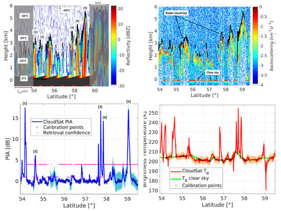
The methodology is demonstrated with a case study which occurred on the 2 January 2009 in the Gulf of Alaska (Figure 2). The profiles of CPR reflectivity (top left panel) clearly show a sequence of cells that tend to become increasingly taller (up to more than 5 km and to temperatures colder than −40 °C) when moving closer to the coast (located at approximately 59.5° N). The cells are isolated with gaps of clear sky, where the CALIOP backscattering profiles (Panel b) show very strong ocean surface backscattering. These profiles can be assumed to be “cloud-free” and can be used to calibrate the PIAs and the s. The 2B-CLDCLASS product (Panel c) labels these precipitating clouds mainly as stratus (St) and stratocumulus (Sc), with the tallest structures classified as nimbostratus (Ns) clouds. Note that shallow cumuliform snowfall is characteristic over the ice-free ocean, where it is typically triggered by cold outbreaks [3,25].
Regions over land and with 2 m temperature above freezing (grey shaded areas in the top panel of Figure 2) are excluded from our analysis, because in such areas, the interpretation of the PIA and the signal is complicated by the uncertainties of the surface emissivity and of the rain attenuation. The environment is quite dry with IWV around 5 kg/m2 (top panel in Figure 3); the 2C-SNOW-PROFILE product retrieves snowfall rates (SR) exceeding 1 mm/h in most of the cells and reaching 3 mm/h; similarly, SWP reaches up to 5 kg/m2 in correspondence to the cell at 59° N.
CloudSat PIA estimates from the surface reference technique [42] and s are shown in Figure 3b,c. The black dots indicate the points used as a calibration reference, where the hydrometeor PIA is adjusted to be zero [40]; similarly, such points are used to calibrate the ocean emissivities computed with the TESSEM model so that the clear sky s corresponding to the ECMWF profiles match the CloudSat s. Note that such “calibration intervals” have widths widely changing depending on the scene; they may be quite frequent in convective snow scenarios, but it can be extremely difficult to find “calibration intervals’’ for several hundred kilometers in the presence of deep nimbostratus clouds. Generally, there is a good correlation between enhanced PIAs and increased s. Several (5) cells have two-way hydrometeor PIA exceeding 5 dB and are flagged by the 2C-SNOW-PROFILE product as producing snowfall at the ground; correspondingly, s show strong (emission) enhancement (up to 254 K for the cell located at 57.7° N, i.e., a warming effect of ), for all cells but the one reaching 5 km in depth and 20 dBZ in reflectivities located at around 59.1° N, which shows a strong depression down to 170.5 K. Since the clear sky values are around 205 K, this corresponds to −35 K. This is a sign of strong scattering, likely caused by large density ice; the retrieved SWP is also quite exceptional (5.8 kg/m2), corresponding to the 99.987 percentile within the analysed dataset.
Five measured reflectivities and retrieved snowfall rate profiles exceeding PIAs of 6 dB and with snow at the surface located as shown in Figure 2a and in Figure 3b, demonstrate that, in all cases, reflectivities reach a maximum in the upper portion of the snow cloud and then decrease significantly in the lower troposphere. The 2C-SNOW-PROFILE algorithm clearly interprets such a decrease as sublimation, as highlighted by the snowfall rates that follow the measured reflectivity decrease in the lower levels. PIA and measurements seem to suggest a different interpretation: the measured reflectivity decrease is a result of attenuation caused by SLWC and/or by the snow itself. For the profiles [2] and [4], the strong enhancement, the low values of the maximum reflectivities, and the large drop of reflectivities from the height of maximum to the lowest clutter-free height seem to suggest the presence of embedded SLWC (the DARDAR cloud mask does not identify SLWC at cloud top). On the other hand, for profiles [1], [3] and [5] it is more likely that some of the attenuation could be caused by the snow itself and that it could be partially compensated (in the reflectivity profile but not in the PIA) by multiple scattering, as suggested by [27]; this would explain the smaller drop of the reflectivity in the lower layers compared to the PIA signal. Overall, the retrieval is very uncertain for these profiles, as highlighted by the low values of the retrieval confidence and the large retrieval errors. This example suggests that the presence of SLWC and/or snow attenuation remains a critical component in CPR snow retrievals.
4. Radiative Transfer Simulations
Simulations of s and PIAs are performed for different combiations of SWPs and LWPs. The deep profile [5] is used as a reference; the snow water content profile retrieved from the 2C-SNOW-PROFILE (modified to be constant below the maximum value reached at circa 4 km) is used as the shape of the profile, which is then modulated to produce any given SWP. The LWP is introduced as a 250 m thick layer. For the profile [5], the DARDAR product does not identify any SLWC at cloud top; therefore, the SLWC is positioned as embedded in the snow layer and located at half the cloud top height (identified by the black line in Figure 2).
To start with, we consider the effect of SLW and snow separately. The sensitivity of s and two-way PIAs to SLW-LWP and SWP is shown in Figure 5. SLW is roughly producing 8 dB of two-way attenuation for each kg/m2; the (warming) sensitivity of to LWP is quite large [118 K/(kg/m2)] at LWP = 0 kg/m2, decreases to 37.8 K/(kg/m2) at LWP = 0.5 kg/m2 and tends to saturate at large values (e.g., it is 10.5 K/(kg/m2) at LWP = 1 kg/m2). Attenuation due to snow is much more difficult to predict, but recent works have clearly demonstrated that, for reflectivities exceeding 10 dBZ [50,55], it cannot be neglected. Different scattering models predict two-way attenuation in a large range of values, e.g., ranging from 0.77 dB to 2.5 dB for each kg/m2 of SWP for the LS15A0.0 and the LS15A0.2, respectively. The corresponding (cooling) sensitivity is −2.3 K/(kg/m2), −3.9 K/(kg/m2) and −7.1 K/(kg/m2) at SWP = 0 kg/m2, peaking at −3.9 K/(kg/m2) −7.6 K/(kg/m2) and −12.7 K/(kg/m2) at circa SWP = 1 kg/m2 for the LS15A0.0, HW14 and LS15A0.2 models, respectively, and then decreasing again at larger SWPs.
Now we consider different combinations of LWPs and SWPs (Figure 6). There are two counteracting effects: the cooling induced by the scattering effect of snow and the warming produced by the SLWC emission. The snow cooling effect is critically dependent on the snow microphysics, with fluffy aggregates (left panel, model LS15A0.0) generally being less efficient in counteracting the SLWC warming (note the bending upwards of the isolines in the right panel for the LS15A0.2 model). Furthermore, because of the larger contribution of snow attenuation, much larger PIAs are attainable for the LS15A0.2 model. The black dots correspond to the best (SWP,LWP) pairs matching the different and PIA pairs measured for the case study (see Figure 3); the larger markers correspond to the five profiles shown in Figure 4. A Euclidean distance re-normalised by a standard deviation of 2 K and of 1 dB for the s and PIAs is used. Different solutions are found for different snow scattering models; for the LS15A0.0 model, a solution for profiles [1], [3] and [5] (diamond, hexagon, triangle) is found only for SWP > 10 kg/m2 (not shown, because deemed unrealistically large). As previously guessed, profile [2] and [4] (square and circle) seem to be dominated by the presence of large SLWC amounts, whereas the other three profiles seem to require the presence of large amounts of heavily rimed particles. Note that the SWP values retrieved for the five profiles from the 2C-SNOW-PROFILE are 1.27, 0.13, 1.33, 0.19 and 5.8 kg/m2, respectively (red symbols in Figure 6). While for profile [2], it is realistically to think of small SWP values (the best solution for all scattering models is SWP = 0.0 kg/m2), the same conclusion cannot be drawn for profile [4], which is characterised by a reflectivity exceeding 10 dBZ. For such a profile, the matching method provides a (SWP,LWP) solution of (5.4,1.1) kg/m2 and (2.1,1.1) kg/m2 for model LS15A0.0 and model LS15A0.2, respectively.
The impact of the position of the SLWC layer is illustrated in Figure 7, by embedding SLW layers instead of at cloud top in the middle of the cloud system corresponding to profile [5]. Because of the much colder temperature of the cloud, SLWC layers located at cloud top instead of embedded tend to produce colder s when large LWP are present. The effect is compensated with increasing SWP, because of the shadowing effect of the SLWC layer on the scattering depressions caused by the underlying ice.
5. Statistical Results and Discussion
The entire 2008 CloudSat dataset has been used to characterize snow profiles over the ice-free ocean. The total snowfall occurrence (conditional mean snow rate) over ice-free ocean is 48% (0.20 mm/h), while over sea ice it is 52% (0.17 mm/h): overall, snowfall over ice-free ocean represents 52% of the amount for snowfall over the ocean. Figure 8 shows the ice-free ocean global maps of snowfall occurrence (normalised to the total snowfall occurrences over ocean, including sea ice) and of the mean annual snowfall rate, obtained from the 2C-SNOW-PROFILE CPR product. Distinct snowfall occurrence maxima exceeding 30% can be noted in the Northern Atlantic Ocean West of Greenland in the Barents Sea, in the southern Bering Sea, and the Southern Hemispheric pan-oceanic region, between 60° S and 70° S. CloudSat-generated snowfall rates are also partitioned between different regions, and the highest snowfall rates exceeding 500mm/y−1 are found in the regions previously mentioned. A similar pattern has been found in a more extensive analysis (2006–2010) by [3]. It is worth mentioning that this snowfall climatology is subject to the CloudSat CPR limitations previously mentioned (attenuation, ground clutter, although limited over ocean, limited temporal and spatial coverage, and 2C-SNOW-PROFILE algorithm assumptions).
Of the snowy profiles over the ice-free ocean 67% and 28% are classified as Sc/Cu or Ns, whereas 55% (45%) have (have no) SLWC at cloud top with a preponderance of profiles without (with) SLWC at cloud top for Ns (Sc/Cu). Sc/Cu clouds occur predominatly at lower IWV contents whereas Ns tend to produce higher SWP (see Figure 9).
The probability distribution functions (pdfs) of PIA (Figure 10, left panel) show that PIA is certainly not negligible (larger than 3 dB) for roughly 6% of the snowy profiles, with a slightly greater likelihood of larger percentage for Sc/Cu clouds. The most extreme attenuation cases correspond to profiles without SLWC at cloud top. This is related to the fact that SLWC at cloud top are usually associated with lower SWP values [5]. Note that this does not exclude the fact that profiles with embedded SLWC layers can actually produce large attenuation; such profiles are indeed those where riming is expected to occur, with rimed particles generally producing much larger attenuation than fluffy aggregates.
pdfs show a mode close to zero with a very small fraction of values smaller than 0 K: depressions of more than 5 K occur in general for less than 1% of the profiles, except for Ns w/o SLW, for which the occurrence exceeds 2.5%. Large warming (of the order of 40 K) on the other hand are not that unusual. The −35 K value corresponding to profile [5] in Figure 2 appears, therefore, to be quite exceptional.
Two-dimensional (PIA,s) histograms are depicted in the left (right) panel of Figure 11 for snow cases with SWP lower (higher) than 1 kg/m2. The latter profiles represent less than 3% of the occurrences (see Figure 11), but correspond to the highest snow-rates where current CloudSat products are affected by strong underestimation [26,56]. For low SWP, there is a continuous trend of increasing s with the PIA, as expected by the dominant role played by the SLW: increasing values of LWP produce larger and larger PIAs and higher and higher s till saturation is reached. Note that some of the negative values of s in the left panel correspond to low PIA values and are very likely caused by errors in the determination of the “clear sky” baseline for the s, which represents a critical step for any interpretation of the s. This requires unbiased estimates of the surface emissivities and of the integrated water vapour. When considering values of SWP larger than 1 kg/m2, the increase of s with increasing PIAs is muted by the compensating effect of ice scattering which partly counterbalances the SLWC warming (e.g., compare the median curves in the left and in the right panels).
6. Conclusions
Accurate measurements of solid precipitation at high-latitude locations remain a critical gap in atmospheric science studies. Spaceborne radars (currently the CloudSat CPR and the GPM-DPR) represent the backbone of the satellite observing system [18,19], although passive microwave (PMW) radiometry is needed to achieve better temporal and spatial coverage. Thanks to their excellent sensitivity, W-band radars remain by far the best tool for snow detection [26]. Quantitative retrievals of snow at W-band, however, remain highly uncertain, with attenuation correction representing a major roadblock [56], mainly because of the uncertainty in the identification of SLWC layers.
The preliminary analysis carried out in this work highlights the potential role of the CloudSat radiometric mode for a better characterization and quantification of snow falling over the ice-free ocean, which has well constrained emissivity and backscattering properties. Falling snow generally cohabits with SLWC layers, with both hydrometeors contributing to non-negligible attenuation at W-band and above. Therefore, accurate quantitative estimates of snow at W-band (or at higher frequencies) require one to account for such attenuation. This is paramount because such estimates are used for calibrating PMW radiometer algorithms [4,6,26,57]. More radiative transfer simulations and synthetic retrievals are recommended in order to asses the improvement in the snow retrieval performances when radiometric modes are available.
The understanding of the SLWC vs. snow attenuation partitioning is not only relevant for properly correcting W-band attenuation (and, as a result, for improving global snowfall climatology), but also to fully understand the impact of SLWC in the presence of snowfall on the PMW spectral signature. Furthermore, refs. [4,58] highlighted that, at high latitudes in cold/dry conditions, the emission signal in the snowfall-sensing high-frequency channels (>90 GHz) due to SLWC at the cloud top is clearly evident in shallow snowfall clouds, while the interpretation of the signal due to embedded SLWC, associated with deeper clouds, is more complex. In [5,57], an all-surface PMW snowfall retrieval algorithm has been developed where the Cloudsat/Calipso-based SLW is used to account for the impact of SLWC on s. However, only the contribution of SLW at the cloud top is considered, when Cloudsat/Calipso-based SLW identification is more certain. In the present study, it has been evidenced that the impact of embedded SLWC on s can be very significant.
The possibility of including the CPR passive mode could be very useful to improve the detection of SLW embedded in the clouds. While the PIAs estimated from the reduction of the ocean surface backscattering return are generally proportional to the total optical thickness, the brightness temperatures react differently to the different hydrometeor: the SLWC optical thickness is associated to absorption/emission (thus causing warming), while the snow optical thickness is mainly linked to scattering (thus causing cooling). The combined information of perfectly co-located s and PIA (possible if the same antenna is shared by the radar and the radiometer) should therefore help in disentangling the two contributions. The main difficulty stems from the availability of “clear-sky” pixels, that can provide a baseline for the s. This issue is particularly critical for large stratiform systems which do not present gaps like convective systems. For such systems, the radiometric mode is therefore expected to have a greater impact.
The interpretation of the is also complicated by the variability of snow scattering properties and by the location of the SLWC, which, even with co-located lidar observations, may remain highly uncertain. Part of these ambiguities can be mitigated by the use of radar at higher frequency in the G-band (i.e., from 110 to 300 GHz, [59]), like recently implemented by [60]. At such frequencies, there is an enhanced sensitivity in the PIAs both to SLWC and snow attenuation, while s tend to produce much stronger cooling due to ice scattering (see thin lines with diamonds in Figure 5).
Future missions specifically targeting high latitude precipitation should therefore consider not only a multi-frequency approach [7], but also the inclusion of radiometric modes at W-band and above, which will be particularly useful over ice-free ocean surfaces to better constrain the liquid and snow water paths of snow-bearing clouds. One of the main difficulties in the interpretation of brightness temperature (and, partially, in the determination of PIAs) resides in the characterisation of the background conditions, mainly the water vapor profiles and the state of the ocean surface (e.g., sea surface temperature and wind), essential for the computation of the “clear sky” baseline and for the surface normalised backscattering cross section [41]. Therefore, it is highly recommended to fly such missions in constellation with passive microwave sensors (e.g., like the Copernicus Imaging Microwave Radiometer (CIMR), [61]) capable of a thorough characterization of the state of the surface at high resolution and, potentially, in nearly coincident time. The possibility of including: (1) multiple tones in the 183 GHz water vapour band as proposed by [62,63] should also be considered to better constrain the tropospheric water vapor and (2) Doppler capabilities like discussed in [7] to be able to discriminate different degrees of riming [64]. Note that such a system could indeed be very beneficial also for the characterization of snow over land and sea-ice regions. A detailed study of the benefit of such a mission for quantitative snow retrievals will be the topic of future research.
Author Contributions
A.B. did the CloudSat analysis and drafted the paper G.P. wrote the introduction, contributed to the analysis of results, and reviewed the paper. Both authors have read and agreed to the published version of the manuscript.
Funding
The work was funded by the ESA-project “Raincast” contract: 4000125959/18/NL/NA.
Acknowledgments
This research used the ALICE High Performance Computing Facility at the University of Leicester.
Conflicts of Interest
The authors declare no conflict of interest. The funders had no role in the design of the study; in the collection, analyses, or interpretation of data; in the writing of the manuscript, or in the decision to publish the results.
Appendix A. List of Acronyms
- AMSR-E: Advanced Microwave Scanning Radiometer for EOS
- CALIOP: Cloud-Aerosol Lidar with Orthogonal Polarization
- CIMR: Copernicus Imaging Microwave Radiometer
- CPR: Cloud Profiling Radar
- Cu: Cumulus
- DARDAR: RaDAR liDAR
- DPR: Dual-frequency Precipitation Radar
- EarthCARE: Earth Clouds, Aerosols and Radiation Explorer
- ECMWF: European Centre for Medium Range Forecast
- GPM: Global Precipitation Measurements
- IR: Infrared
- IWV: Integrated Water Vapour
- LWP: Liquid Water Path
- MW: MicroWave
- Ns: Nimbostratus
- PIA: Path Integrated Attenuation
- PMW: Passive MicroWave
- Sc: Stratocumulus
- SLW: Supercooled Liquid Water
- SLWC: Supercooled Liquid Water Content
- SST: Sea Surface Temperature
- TESSEM: Tool to Estimate Sea Surface Emissivity from Microwave to sub-M
- TB: Brightness Temperature
- VIS: Visible
References
- Levizzani, V.; Laviola, S.; Cattani, E. Detection and Measurement of Snowfall from Space. Remote Sens. 2011, 3, 145–166. [Google Scholar] [CrossRef] [Green Version]
- Wang, Y.; Liu, G.; Seo, E.K.; Fu, Y. Liquid water in snowing clouds: Implications for satellite remote sensing of snowfall. Atmos. Res. 2013, 131, 60–72. [Google Scholar] [CrossRef]
- Kulie, M.S.; Milani, L.; Wood, N.B.; Tushaus, S.A.; Bennartz, R.; L’Ecuyer, T.S. A Shallow Cumuliform Snowfall Census Using Spaceborne Radar. J. Hydrometeorol. 2016, 17, 1261–1279. [Google Scholar] [CrossRef]
- Panegrossi, G.; Rysman, J.F.; Casella, D.; Marra, A.C.; Sanò, P.; Kulie, M.S. CloudSat-Based Assessment of GPM Microwave Imager Snowfall Observation Capabilities. Remote Sens. 2017, 9, 1263. [Google Scholar] [CrossRef] [Green Version]
- Rysman, J.F.; Panegrossi, G.; Sanò, P.; Marra, A.; Dietrich, S.; Milani, L.; Kulie, M. SLALOM: An All-Surface Snow Water Path Retrieval Algorithm for the GPM Microwave Imager. Remote Sens. 2018, 10, 1278. [Google Scholar] [CrossRef] [Green Version]
- Skofronick-Jackson, G.; Kulie, M.; Milani, L.; Munchak, S.J.; Wood, N.B.; Levizzani, V. Satellite Estimation of Falling Snow: A Global Precipitation Measurement (GPM) Core Observatory Perspective. J. Appl. Meteorol. Climatol. 2019, 58, 1429–1448. [Google Scholar] [CrossRef]
- Battaglia, A.; Kollias, P.; Dhillon, R.; Roy, R.; Tanelli, S.; Lamer, K.; Grecu, M.; Lebsock, M.; Watters, D.; Mroz, K.; et al. Spaceborne Cloud and Precipitation Radars: Status, Challenges, and Ways Forward. Rev. Geophys. 2020, 58, e2019RG000686. [Google Scholar] [CrossRef]
- Bennartz, R.; Bauer, P. Sensitivity of microwave radiances at 85–183 GHz to precipitating ice particles. Radio Sci. 2003, 38. [Google Scholar] [CrossRef]
- Skofronick-Jackson, G.; Johnson, B.T. Surface and atmospheric contributions to passive microwave brightness temperatures for falling snow events. J. Geophys. Res. 2011, 116, D02213. [Google Scholar] [CrossRef]
- You, Y.; Wang, N.Y.; Ferraro, R.; Meyers, P. A Prototype Precipitation Retrieval Algorithm over Land for ATMS. J. Hydrometeorol. 2016, 17, 1601–1621. [Google Scholar] [CrossRef]
- Skofronick-Jackson, G.; Kirschbaum, D.; Petersen, W.; Huffman, G.; Kidd, C.; Stocker, E.; Kakar, R. The Global Precipitation Measurement (GPM) mission’s scientific achievements and societal contributions: Reviewing four years of advanced rain and snow observations. Quart. J. R. Meteor. Soc. 2018, 144, 27–48. [Google Scholar] [CrossRef] [PubMed] [Green Version]
- Tanelli, S.; Durden, S.L.; Im, E.; Pak, K.S.; Reinke, D.G.; Partain, P.; Haynes, J.M.; Marchand, R.T. CloudSat’s Cloud Profiling Radar After Two Years in Orbit: Performance, Calibration, and Processing. IEEE Trans. Geosci. Remote Sens. 2008, 46, 3560–3573. [Google Scholar] [CrossRef]
- Illingworth, A.J.; Barker, H.W.; Beljaars, A.; Ceccaldi, M.; Chepfer, H.; Clerbaux, N.; Cole, J.; Delanoë, J.; Domenech, C.; Donovan, D.P.; et al. The EarthCARE Satellite: The Next Step Forward in Global Measurements of Clouds, Aerosols, Precipitation, and Radiation. Bull. Am. Met. Soc. 2015, 96, 1311–1332. [Google Scholar] [CrossRef] [Green Version]
- Kulie, M.S.; Bennartz, R. Utilizing Spaceborne Radars to Retrieve Dry Snowfall. J. Appl. Meteorol. Climatol. 2009, 48, 2564–2580. [Google Scholar] [CrossRef] [Green Version]
- Hiley, M.J.; Kulie, M.S.; Bennartz, R. Uncertainty Analysis for CloudSat Snowfall Retrievals. J. Appl. Meteorol. Climatol. 2011, 50, 399–418. [Google Scholar] [CrossRef]
- Wood, N.B.; L’Ecuyer, T.S. Level 2C Snow Profile Process Description and Interface Control Document, Version 0. CloudSat Project: A NASA Earth System Science Pathfinder Mission. 2013. Available online: http://www.cloudsat.cira.colostate.edu/sites/default/files/products/files/2C-SNOW-PROFILE_PDICD.P_R04.20130210.pdf (accessed on 19 June 2020).
- Bennartz, R.; Fell, F.; Pettersen, C.; Shupe, M.D.; Schuettemeyer, D. Spatial and temporal variability of snowfall over Greenland from CloudSat observations. Atmos. Chem. Phys. 2019, 19, 8101–8121. [Google Scholar] [CrossRef] [Green Version]
- Liu, G. Satellite Precipitation Measurement; Advances in Global Change Research, 67, Chapter Radar Snowfall Meausurements; Springer Nature: Cham, Switzerland, 2020; Volume 1, pp. 277–296. [Google Scholar] [CrossRef]
- Kulie, M.; Milani, L.; Wood, N.; L’Ecuyer, T. Satellite Precipitation Measurement; Advances in Global Change Research, 69, Chapter Global Snowfall Detection and Measurement; Springer Nature: Cham, Switzerland, 2020; Volume 2, pp. 277–296. [Google Scholar] [CrossRef]
- Liu, G. A database of microwave single-scattering properties for nonspherical ice particles. Bull. Am. Met. Soc. 2008, 89, 1563–1570. [Google Scholar] [CrossRef] [Green Version]
- Mätzler, C.; Morland, J. Advances in Surface-Based Radiometry of Atmospheric Water; Technical Report; University of Bern: Bern, Switzerland, 2008. [Google Scholar]
- Behrangi, A.; Stephens, G.; Adler, R.F.; Huffman, G.J.; Lambrigtsen, B.; Lebsock, M. An Update on the Oceanic Precipitation Rate and Its Zonal Distribution in Light of Advanced Observations from Space. J. Clim. 2014, 27, 3957–3965. [Google Scholar] [CrossRef] [Green Version]
- Milani, L.; Kulie, M.S.; Casella, D.; Dietrich, S.; L’Ecuyer, T.S.; Panegrossi, G.; Porcù, F.; Sanò, P.; Wood, N.B. CloudSat snowfall estimates over Antarctica and the Southern Ocean: An assessment of independent retrieval methodologies and multi-year snowfall analysis. Atmos. Res. 2018, 213, 121–135. [Google Scholar] [CrossRef]
- Palerme, C.; Kay, J.E.; Genthon, C.; L’Ecuyer, T.; Wood, N.B.; Claud, C. How much snow falls on the Antarctic ice sheet? Cryosphere 2014, 8, 1577–1587. [Google Scholar] [CrossRef] [Green Version]
- Kulie, M.S.; Milani, L. Seasonal variability of shallow cumuliform snowfall: A CloudSat perspective. Quart. J. R. Meteor. Soc. 2018, 144, 329–343. [Google Scholar] [CrossRef] [Green Version]
- Mróz, K.; Montopoli, M.; Panegrossi, G.; Baldini, L.; Battaglia, A.; Kirstetter, P. Quality assessment of spaceborne active and passive microwave snowfall products over the continental United States. J. Hydrometeorol. 2020. submitted. [Google Scholar]
- Matrosov, S.Y.; Battaglia, A. Influence of multiple scattering on CloudSat measurements in snow: A model study. Geophys. Res. Lett. 2009, 36, L12806. [Google Scholar] [CrossRef] [Green Version]
- Casella, D.; Panegrossi, G.; Sanò, P.; Marra, A.C.; Dietrich, S.; Johnson, B.T.; Kulie, M.S. Evaluation of the GPM-DPR snowfall detection capability: Comparison with CloudSat-CPR. Atmos. Res. 2017, 197, 64–75. [Google Scholar] [CrossRef]
- Palerme, C.; Claud, C.; Wood, N.B.; L’Ecuyer, T.; Genthon, C. How Does Ground Clutter Affect CloudSat Snowfall Retrievals Over Ice Sheets? IEEE Geosci. Remote Sens. Lett. 2019, 16, 342–346. [Google Scholar] [CrossRef] [Green Version]
- Matrosov, S.Y. Comparative Evaluation of Snowfall Retrievals from the CloudSat W-band Radar Using Ground-Based Weather Radars. J. Atmos. Ocean. Technol. 2019, 36, 101–111. [Google Scholar] [CrossRef]
- Pettersen, C.; Kulie, M.S.; Bliven, L.F.; Merrelli, A.J.; Petersen, W.A.; Wagner, T.J.; Wolff, D.B.; Wood, N.B. A Composite Analysis of Snowfall Modes from Four Winter Seasons in Marquette, Michigan. J. Appl. Meteorol. Climatol. 2020, 59, 103–124. [Google Scholar] [CrossRef]
- Lamer, K.; Kollias, P.; Battaglia, A.; Preval, S. Mind-the-gap part I: Accurately locating warm marine boundary layer clouds and precipitation using spaceborne radars. Atmos. Meas. Tech. Discuss. 2020, 13, 2363–2379. [Google Scholar] [CrossRef]
- Battaglia, A.; Delanöe, J. Synergies and complementarities of CloudSat-CALIPSO snow observations. J. Geophys. Res. Atmos. 2013, 118, 721–731. [Google Scholar] [CrossRef] [Green Version]
- Shupe, M.D. Clouds at Arctic Atmospheric Observatories. Part II: Thermodynamic Phase Characteristics. J. Appl. Meteorol. Climatol. 2011, 50, 645–661. [Google Scholar] [CrossRef]
- Lubin, D.; Zhang, D.; Silber, I.; Scott, R.C.; Kalogeras, P.; Battaglia, A.; Bromwich, D.H.; Cadeddu, M.; Eloranta, E.; Fridlind, A.; et al. AWARE: The Atmospheric Radiation Measurement (ARM) West Antarctic Radiation Experiment. Bull. Am. Met. Soc. 2020, 101, E1069–E1091. [Google Scholar] [CrossRef] [Green Version]
- Pettersen, C.; Bennartz, R.; Merrelli, A.J.; Shupe, M.D.; Turner, D.D.; Walden, V.P. Precipitation regimes over central Greenland inferred from 5 years of ICECAPS observations. Atmos. Chem. Phys. 2018, 18, 4715–4735. [Google Scholar] [CrossRef] [Green Version]
- Kneifel, S.; Löhnert, U.; Battaglia, A.; Crewell, S.; Siebler, D. Snow scattering signals in ground-based passive microwave radiometer measurements. J. Geophys. Res. 2010, 115, D16214. [Google Scholar] [CrossRef] [Green Version]
- Ebtehaj, A.M.; Kummerow, C.D. Microwave retrievals of terrestrial precipitation over snow-covered surfaces: A lesson from the GPM satellite. Geophys. Res. Lett. 2017, 44, 6154–6162. [Google Scholar] [CrossRef]
- Takbiri, Z.; Ebtehaj, A.; Foufoula-Georgiou, E.; Kirstetter, P.E.; Turk, F.J. A Prognostic Nested k-Nearest Approach for Microwave Precipitation Phase Detection over Snow Cover. J. Hydrometeorol. 2019, 20, 251–274. [Google Scholar] [CrossRef] [PubMed]
- Lebsock, M.D.; Suzuki, K. Uncertainty Characteristics of Total Water Path Retrievals in Shallow Cumulus Derived from Spaceborne Radar/Radiometer Integral Constraints. J. Atmos. Ocean. Technol. 2016, 33, 1597–1609. [Google Scholar] [CrossRef]
- Battaglia, A.; Kollias, P.; Dhillon, R.; Lamer, K.; Khairoutdinov, M.; Watters, D. Mind-the-gap Part II: Improving quantitative estimates of cloud and rain water path in oceanic warm rain using spaceborne radars. Atmos. Meas. Tech. Discuss. 2020, 13, 4865–4883. [Google Scholar] [CrossRef]
- Leinonen, J.; Lebsock, M.D.; Stephens, G.L.; Suzuki, K. Improved Retrieval of Cloud Liquid Water from CloudSat and MODIS. J. Appl. Meteorol. Climatol. 2016, 55, 1831–1844. [Google Scholar] [CrossRef]
- Winker, D.M.; Pelon, J.; Coakley, J.A., Jr.; Ackerman, S.A.; Charlson, R.J.; Colarco, P.R.; Flamant, P.; Fu, Q.; Hoff, R.M.; Kittaka, C.; et al. The CALIPSO Mission: A global 3D view of aerosols and clouds. Bull. Am. Met. Soc. 2010, 91, 1211–1229. [Google Scholar] [CrossRef]
- Mace, G.G.; Avey, S.; Cooper, S.; Lebsock, M.; Tanelli, S.; Dobrowalski, G. Retrieving Co-Occurring Cloud and Precipitation Properties of Warm Marine Boundary Layer Clouds with A-Train Data. J. Geophys. Res. 2016, 121, 4008–4033. [Google Scholar] [CrossRef] [Green Version]
- Delanoë, J.; Hogan, R.J. Combined CloudSat-CALIPSO-MODIS retrievals of the properties of ice clouds. J. Geophys. Res. Atmos. 2010, 115, D00H29. [Google Scholar] [CrossRef] [Green Version]
- Sassen, K.; Wang, Z. Classifying clouds around the globe with the CloudSat radar: 1-year of results. Geophys. Res. Lett. 2008, 35, L04805. [Google Scholar] [CrossRef]
- Haynes, J.M.; L’Ecuyer, T.S.; Stephens, G.L.; Miller, S.D.; Mitrescu, C.; Wood, N.B.; Tanelli, S. Rainfall retrieval over the ocean with spaceborne W-band radar. J. Geophys. Res. Atmos. 2009, 114, D00A22. [Google Scholar] [CrossRef]
- Kummerow, C. On the accuracy of the Eddington approximation for radiative transfer in the microwave frequencies. J. Geophys. Res. 1993, 98, 2757–2765. [Google Scholar] [CrossRef]
- Prigent, C.; Aires, F.; Wang, D.; Fox, S.; Harlow, C. Sea-surface emissivity parametrization from microwaves to millimetre waves. Quart. J. R. Meteor. Soc. 2017, 143, 596–605. [Google Scholar] [CrossRef]
- Tridon, F.; Battaglia, A.; Kneifel, S. How to estimate total differential attenuation due to hydrometeors with ground-based multi-frequency radars? Atmos. Meas. Tech. Discuss. 2020, 2020, 1–29. [Google Scholar] [CrossRef]
- Turner, D.D.; Kneifel, S.; Careddu, M.P. An Improved Liquid Water Absorption Model at Microwave Frequencies for Supercooled Liquid Water Clouds. J. Atmos. Ocean. Technol. 2016, 33, 33–44. [Google Scholar] [CrossRef]
- Mróz, K.; Battaglia, A.; Kneifel, S.; von Terzi, L.; Karrer, M.; Ori, D. Linking rain into ice microphysics across the melting layer in stratiform rain: A closure study. Atmos. Meas. Tech. Discuss. 2020. preprint. [Google Scholar] [CrossRef]
- Leinonen, J.; Szyrmer, W. Radar signatures of snowflake riming: A modeling study. Earth Space Sci. 2015, 2, 346–358. [Google Scholar] [CrossRef]
- Hogan, R.J.; Westbrook, C.D. Equation for the microwave backscatter cross section of aggregate snowflakes using the Self-Similar Rayleigh-Gans Approximation. J. Atmos. Sci. 2014, 71, 3292–3301. [Google Scholar] [CrossRef] [Green Version]
- Protat, A.; Rauniyar, S.; Delanoë, J.; Fontaine, E.; Schwarzenboeck, A. W-Band (95 GHz) Radar Attenuation in Tropical Stratiform Ice Anvils. Available online: https://journals.ametsoc.org/jtech/article/36/8/1463/343564/W-Band-95-GHz-Radar-Attenuation-in-Tropical (accessed on 9 October 2020).
- Cao, Q.; Hong, Y.; Chen, S.; Gourley, J.J.; Zhang, J.; Kirstetter, P.E. Snowfall Detectability of NASA’s CloudSat: The First Cross-Investigation of its 2c-Snow-Profile Product and National Multi-Sensor Mosaic QPE (NMQ) Snowfall Data. Progress Electromagn. Res. 2014, 148, 55–61. [Google Scholar] [CrossRef]
- Rysman, J.F.; Panegrossi, G.; Sanò, P.; Marra, A.C.; Dietrich, S.; Milani, L.; Kulie, M.S.; Casella, D.; Camplani, A.; Claud, C.; et al. Retrieving Surface Snowfall With the GPM Microwave Imager: A New Module for the SLALOM Algorithm. Geophys. Res. Lett. 2019, 46, 13593–13601. [Google Scholar] [CrossRef]
- Edel, L.; Rysman, J.F.; Claud, C.; Palerme, C.; Genthon, C. Potential of Passive Microwave around 183 GHz for Snowfall Detection in the Arctic. Remote Sens. 2019, 11, 2200. [Google Scholar] [CrossRef] [Green Version]
- Battaglia, A.; Westbrook, C.D.; Kneifel, S.; Kollias, P.; Humpage, N.; Löhnert, U.; Tyynelä, J.; Petty, G.W. G band atmospheric radars: New frontiers in cloud physics. Atmos. Meas. Tech. 2014, 7, 1527–1546. [Google Scholar] [CrossRef] [Green Version]
- Roy, R.J.; Lebsock, M.; Millán, L.; Cooper, K.B. Validation of a G-Band Differential Absorption Cloud Radar for Humidity Remote Sensing. J. Atmos. Ocean. Technol. 2020, 37, 1085–1102. [Google Scholar] [CrossRef] [Green Version]
- Kilic, L.; Prigent, C.; Aires, F.; Boutin, J.; Heygster, G.; Tonboe, R.T.; Roquet, H.; Jimenez, C.; Donlon, C. Expected Performances of the Copernicus Imaging Microwave Radiometer (CIMR) for an All-Weather and High Spatial Resolution Estimation of Ocean and Sea Ice Parameters. J. Geophys. Res. Oceans 2018, 123, 7564–7580. [Google Scholar] [CrossRef] [Green Version]
- Battaglia, A.; Kollias, P. Evaluation of differential absorption radars in the 183 GHz band for profiling water vapour in ice clouds. Atmos. Meas. Tech. 2019, 12, 3335–3349. [Google Scholar] [CrossRef] [Green Version]
- Millán, L.; Roy, R.; Lebsock, M. Assessment of global total column water vapor sounding using a spaceborne differential absorption radar. Atmos. Meas. Tech. Discuss. 2020, 13, 5193–5205. [Google Scholar] [CrossRef]
- Mason, S.L.; Chiu, C.J.; Hogan, R.J.; Moisseev, D.; Kneifel, S. Retrievals of Riming and Snow Density From Vertically Pointing Doppler Radars. J. Geophys. Res. Atm. 2018, 123, 13807–13834. [Google Scholar] [CrossRef] [Green Version]
Figure 1.
Flow chart illustrating the methodology followed to: first, identify snow events; then, classify the profiles within the event as snow-free w/ and w/o supercooled liquid water clouds (SLWC) and as snowy w/ and w/o SLWC; finally, compute , i.e., the variation in snowfall conditions compared to the clear sky reference (see text for details). Rhomboid boxes correspond to the CloudSat satellite products used in the analysis.

Figure 2.
Case study of 2 January 2009. (a) CPR reflectivity. (b) Cloud-Aerosol Lidar with Orthogonal Polarization (CALIOP) backscattering. (c) cloud classification. NC = No cloud; Ci = cirrus; As = Altostratus; Ac = Altocumulus; St = Stratus; Sc = Stratocumulus; Cu = Cumulus; Ns = Nimbostratus; DC = Deep Convection. Note that no Dc, Cu, Ac and Ci are present in this scene. Red points correspond to SLWC as identified by the RaDAR liDAR (DARDAR) mask. In all panels, the black line corresponds to the top of the tallest cloud layer, as identified by the radar.

Figure 3.
For the case study shown in Figure 2: (a) integrated water vapour (IWV), surface snowfall rate (SR) and path integrated attenuation (PIA), the snow water path (SWP); (b) CloudSat hydrometeor path integrated attenuation (PIA) adjusted to have zero mean for the calibration intervals marked as black dots; (c) CloudSat s. Shadings correspond to measurements uncertainties as reported in the 2C-SNOW-PROFILE product. Retrieval confidence range from 0 (no confidence) to 4 (high confidence). The reflectivity profiles labelled as [1], ⋯, [5], are shown in Figure 4.

Figure 4.
Profiles of reflectivities (left) and snowfall rates (right) producing maximum PIA for the event shown in Figure 2. Each profile is labelled by a number with its position within the system identified in Figure 2, Panel a. Retrieval confidence (RC) and retrieved surface snowfall rates with corresponding errors computed by the 2C-SNOW-PROFILE algorithm included in the legend demonstrate the high level of uncertainty in the retrieval.

Figure 5.
94 GHz (left) and two-way PIA (right) sensitivity for liquid cloud only (blue line) and for snow-only for different snow scattering models (dashed lines) as a function of liquid water path (LWP) and SWP. SWP is divided by 5 to make scales comparable. Thin lines with diamonds correspond to results for 240 GHz.

Figure 6.
Radiative transfer simulation showing as indicated by the colorbar values with a snow precipitating clouds with different SWP and LWP. The SLWC layer is embedded in the cloud. The clear sky is 203.9 K. The black dots correspond to the best (SWP, LWP) pairs matching the measurements for the case study illustrated in Figure 2, with the black large symbols corresponding to the measurement for the different profiles shown in Figure 4 (with the same symbols), whereas the red symbols on the x-axis represent the SWP for each profile as retrieved in the 2C-SNOW-PROFILE algorithm. Isolines of s and two-way PIAs are plotted as dashed magenta and blue lines.

Figure 7.
Impact of SLWC layer position on . Difference in the between the case of SLWC at cloud top and embedded for the LS15A0.0 model. Isolines of s are plotted as dashed lines.
Figure 7.
Impact of SLWC layer position on . Difference in the between the case of SLWC at cloud top and embedded for the LS15A0.0 model. Isolines of s are plotted as dashed lines.

Figure 8.
CloudSat derived snowfall occurrence (in %) (top) and mean annual snowfall rate (bottom) over ice-free ocean in bins for the 2008 dataset. Snowfall occurrence is defined as the number of snowfall events over ice-free ocean divided by the total number of observations in each grid box.
Figure 8.
CloudSat derived snowfall occurrence (in %) (top) and mean annual snowfall rate (bottom) over ice-free ocean in bins for the 2008 dataset. Snowfall occurrence is defined as the number of snowfall events over ice-free ocean divided by the total number of observations in each grid box.

Figure 9.
Frequency histograms of the 2008 snow profiles for different integrated water path (IWV) (left) and SWP (right) classes.
Figure 9.
Frequency histograms of the 2008 snow profiles for different integrated water path (IWV) (left) and SWP (right) classes.

Figure 10.
PIA (left) and (right) pdfs for snowy profiles for different snow cloud types (Ns and Sc+Cu) and with or without SLWC at cloud top. The percentage in the bracket in the legend of the two panels represents the percentage exceeding the 3 dB threshold and −5 K threshold, respectively, as indicated by the shaded grey regions.

Figure 11.
Two-dimensional occurrence histogram in scale (so 1, ⋯, 4 mean 10, counts) of snow profiles for different combinations of PIA and s. Dashed and continuous lines correspond to the median value for the pdf at any given PIA value for the cases without and with SLWC at cloud top, respectively.

© 2020 by the authors. Licensee MDPI, Basel, Switzerland. This article is an open access article distributed under the terms and conditions of the Creative Commons Attribution (CC BY) license (http://creativecommons.org/licenses/by/4.0/).
Share and Cite
MDPI and ACS Style
Battaglia, A.; Panegrossi, G. What Can We Learn from the CloudSat Radiometric Mode Observations of Snowfall over the Ice-Free Ocean? Remote Sens. 2020, 12, 3285. https://doi.org/10.3390/rs12203285
AMA Style
Battaglia A, Panegrossi G. What Can We Learn from the CloudSat Radiometric Mode Observations of Snowfall over the Ice-Free Ocean? Remote Sensing. 2020; 12(20):3285. https://doi.org/10.3390/rs12203285
Chicago/Turabian StyleBattaglia, Alessandro, and Giulia Panegrossi. 2020. "What Can We Learn from the CloudSat Radiometric Mode Observations of Snowfall over the Ice-Free Ocean?" Remote Sensing 12, no. 20: 3285. https://doi.org/10.3390/rs12203285
Note that from the first issue of 2016, this journal uses article numbers instead of page numbers. See further details here.