Detection of Methane Emission from a Local Source Using GOSAT Target Observations
by
 , , and
Akihiko Kuze
1,* ,
,
Nobuhiro Kikuchi
1,
Fumie Kataoka
2,
Hiroshi Suto
1,
Kei Shiomi
1 and
Yutaka Kondo
3 1
Japan Aerospace Exploration Agency, Tsukuba-City, Ibaraki 305-8505, Japan
2
Remote Sensing Technology Center of Japan, Tsukuba-City, Ibaraki 305-8505, Japan
3
National Institute of Polar Research, Tachikawa-City 190-8518, Japan
*
Author to whom correspondence should be addressed.
Remote Sens. 2020, 12(2), 267; https://doi.org/10.3390/rs12020267
Submission received: 14 November 2019
/
Revised: 30 December 2019
/
Accepted: 6 January 2020
/
Published: 13 January 2020
(This article belongs to the Special Issue Remote Sensing of Carbon Dioxide and Methane in Earth’s Atmosphere)
Abstract
:Emissions of atmospheric methane (CH4), which greatly contributes to radiative forcing, have larger uncertainties than those for carbon dioxide (CO2). The Thermal And Near-infrared Sensor for carbon Observation Fourier-Transform Spectrometer (TANSO-FTS) onboard the Greenhouse gases Observing SATellite (GOSAT) launched in 2009 has demonstrated global grid observations of the total column density of CO2 and CH4 from space, and thus reduced uncertainty in the global flux estimation. In this paper, we present a case study on local CH4 emission detection from a single-point source using an available series of GOSAT data. By modifying the grid observation pattern, the pointing mechanism of TANSO-FTS targets a natural gas leak point at Aliso Canyon in Southern California, where the clear-sky frequency is high. To enhance local emission estimates, we retrieved CO2 and CH4 partial column-averaged dry-air mole fractions of the lower troposphere (XCO2 (LT) and XCH4 (LT)) by simultaneous use of both sunlight reflected from Earth’s surface and thermal emissions from the atmosphere. The time-series data of Aliso Canyon showed a large enhancement that decreased with time after its initial blowout, compared with reference point data and filtered with wind direction simulated by the Weather Research and Forecasting (WRF) model.
1. Introduction
Among trace gases in the atmosphere, methane (CH4) contributes significantly to radiative forcing, second only to carbon dioxide (CO2), although its emissions estimates have larger uncertainties than those of CO2. Major anthropogenic source sectors are oil/gas production, coal mining, livestock, landfills, wastewater, and rice cultivation. A better understanding of the distribution and amount of emissions contributes to effective reductions in CH4 emissions. In situ measurements taken on the ground or by aircraft, using such instruments as cavity-ringdown spectrometers, have high accuracy and precision, but the number of observation points is limited. Airborne remote sensing has demonstrated CH4 point-source emissions and their plumes using imaging capabilities [1,2,3]. With its high spatial resolution, these measurements can detect the fine horizontal structure of plumes from individual emission source, but these are temporary. Long-term measurements are needed for more systematic estimates of CH4 emissions. Satellite observations can provide global CH4 data in a long time-series (over a decade) to investigate anthropogenic CH4 emissions. Compared to the wide-spread urban CO2 emissions, such as those from transportation, most anthropogenic CH4 source areas are smaller than a single pixel in satellite footprints. Such areas can be treated as point sources for existing satellite observations. Jacob et al. [4] reviewed the value of present, future, and proposed satellite observations to better quantify and understand CH4 emissions through inverse analyses from the global scale down to the scale of point sources.
The Scanning Imaging Absorption Spectrometer for Atmospheric CHartographY (SCIAMACHY) is the first spectrometer to observe both CO2 and CH4 form space [5]. After its operation in April 2012 and prior to the launch of the Orbiting Carbon Observatory-2 (OCO-2) for CO2 in 2014, TanSAT for CO2 in 2015, GHGSat for CH4 in 2016, TROPOspheric Monitoring Instrument (TROPOMI) onboard the Sentinel-5 Precursor satellite for CH4 in 2017, and OCO-3 onboard International Space Station (ISS) for CO2 in 2019, the Greenhouse gases Observing SATellite (GOSAT) was the only instrument that could provide CO2 and CH4 column amounts, which are sensitive to the surface from space [6,7,8,9,10,11,12]. GOSAT has demonstrated global grid observation of total column density of CO2 and CH4 from space, and thus has reduced the uncertainty in global flux estimation.
Missions with high spectral resolution for measuring thermal emission include the Atmospheric Infrared Sounder (AIRS) onboard the Earth Observing System (EOS) PM spacecraft, the Tropospheric Emission Spectrometer (TES) onboard the EOS Aura, the Infrared Atmospheric Sounding Interferometer (IASI) onboard Metop satellite, and the Cross-track Infrared Sounder (CrIS) onboard the Suomi National Polar-orbiting Partnership Project (SNPP). They can provide vertical profile information but do not have sufficient sensitivity for enhancements near the surface [13,14,15,16].
As summarized in Table 1, GOSAT is the only nadir-viewing mission that can observe reflected and scattered solar light with two linear polarizations and thermal emission simultaneously. An individual linear polarization band include information on highly polarized scattering by particles. By providing long-term high-resolution spectral data, TANSO-FTS is a pathfinder for subsequent missions and it also provides information to better understand radiative transfer.
However, the grid scan mode covers only 0.1% of Earth’s surface and has missed most CH4 point sources. Turner et al. and Sheng et al. estimated CH4 emissions from North America from different source sectors from sparse sampling data [17,18]. To capture all CH4 emissions, the satellite footprint must cover the point source area. In this study, we modified the pointing pattern locally and retrieved the columnar densities of lower troposphere (LT) CH4 and CO2 by simultaneous use of reflected shortwave-infrared (SWIR) solar light and thermal infrared (TIR) emissions. This paper describes how a local CH4 emission could be detected using existing GOSAT functionalities and wind simulation. We also discuss the possible causes of uncertainty in the local flux estimates and suggest possibilities that might reduce such uncertainties using imaging capabilities on the local flux estimate through satellite data.
2. Data Acquisition and Analytical Dataset for Local Emission Detection
2.1. GOSAT Observations
GOSAT carries the Thermal And Near-infrared Sensor for carbon Observation Fourier-Transform Spectrometer (TANSO-FTS), which simultaneously observes both reflected SWIR solar light and TIR emissions with a single FTS mechanism. Table 2 lists the principal specifications of the GOSAT orbit and the TANSO-FTS spectral band. As described in Table 3, it measures narrow spectral bands at 0.76 m for oxygen (O2), 1.6 m for CO2 and CH4, and 2.0 m for CO2, with a spectral sampling interval of 0.2 cm−1. It also has a wide spectral band to measure thermal emissions from Earth’s surface and atmosphere, including CO2 and CH4. The reflected SWIR solar light passes through Earth’s troposphere, reflects over the surface, and then returns to space. The O2 A band at 0.76 m provides the surface pressure (Psurf). Two linear polarization bands provide information on light-path modification and make accurate remote sensing possible, even under aerosol and thin-cloud contaminated conditions. To maximize the optical throughput of FTS, GOSAT has a circular instantaneous field of view (IFOV) of 15.8 mrad to collect enough photons to improve the signal-to-noise ratio (SNR). The footprint is 10.5 km in diameter for nadir observations.
2.2. Targeting Point Sources
TANSO-FTS has a two-axis agile pointing system, which allows cross-track (CT) and along-track (AT) motions of ±35° and ±20°, respectively, and compensates for the satellite image-motion during interferogram acquisition. It was originally designed for grid scan observations and viewing onboard calibration sources. It takes 4 s to acquire a single interferogram and 0.6 s for pointing and turnaround of the FTS mechanism. For the first six years of GOSAT operations, TANSO-FTS operated mainly in three-point CT scan mode to monitor global CO2 and CH4 with a three-day revisit cycle, using the primary part of the redundant pointing systems with a grid of about 300 km. After the pointing mechanism was switched from primary to secondary on 26 January 2015, the pointing showed more accurate geolocation and stable settling than the degraded primary system. We decided to make more frequent target observations, by uploading AT and CT pointing angles and observation timing as commands from the ground every day [12]. The pointing bias and its fluctuations have generally been smaller than 0.1°, corresponding to a 1 km surface footprint bias or fluctuations. When a sufficiently strong point source is located within the 10.5 km footprint in nadir, GOSAT can capture total CH4 emissions that spread horizontally and vertically. Over the three-day revisit cycle, data of 56,000 locations are acquired, most of which are grid observations and onboard calibrations. About 1000 locations are allocated to target observations, such as the Total Carbon Column Observing Network (TCCON) validation sites, desert areas for radiometric calibration, megacities, or large emission sources [12,19].
2.3. Derivation of CH4 Partial Column-averaged Density in the Lower Troposphere
Estimation of the CH4 local emission requires the columnar density of the LT CH4 in order to enhance near-surface density and reduce the inflow in the upper atmosphere. Existing GOSAT Level 2 products have provided the column-averaged dry-air mole fractions of CO2 and CH4 (XCO2 and XCH4, respectively), but only from the three SWIR-band data [20,21,22,23,24,25]. The standard deviation of XCO2 and XCH4 are 2.1 ppm or 0.5% and 13 ppb or 0.7%, respectively, compared with the TCCON data. Their biases are −1.48 ppm and −5.9 ppb for XCO2 and XCH4, respectively. Columnar CH4 density is the average value of the LT, upper troposphere (UT), and the stratosphere. Therefore, it is influenced by inflows of CH4 in the UT and the stratosphere from a much wider area. In estimating CH4 emissions from a local point source, it is highly desirable to extract columnar density only of the LT CH4. TIR spectra emitted from CO2 and CH4 contain vertical profile information, due to the temperature gradient. Conventional algorithms for the TIR band have attempted to acquire CO2 and CH4 densities for ten vertical layers in the troposphere, resulting in unstable retrievals due to the uncertainties of radiometric calibrations [26]. In addition, TIR data alone do not contain enough information of near-surface CO2 and CH4, and thus are inadequate for local emission analysis.
We reduced the number of vertical layers for a more robust retrieval [27,28]. We can retrieve the difference between the partial column-averaged dry-air mole fractions of the two individual layers of LT and UT (XCO2 (LT), XCO2 (UT), XCH4 (LT), and XCH4 (UT)) by combining TIR and SWIR spectra data simultaneously, thereby constraining the accurate total column density of XCO2 and XCH4.
We retrieved five vertical layers: two in the troposphere and three in the stratosphere. We used the entire spectral range acquired with the FTS listed in Table 3 including absorption bands of O2 A at 0.76 μm, CO2 and CH4 at 1.6 μm, and CO2 at 2.0 μm, and thermal emission from atmospheric CO2 and CH4. The simultaneous use of two liner polarizations can provide accurate light-path modification under thick aerosol conditions.
The retrieval method is the maximum a posteriori solution found by minimizing a cost function. For reflected solar light, we used the vector equation of radiative transfer for the diffuse components of the Stokes parameters. We define vertical layers of LT and UT not by temperature, but by the retrieved Psurf from individual O2 A band data as retrieved vertical temperature has a larger uncertainty. The pressure-height ranges of the LT and UT were taken as 0.6–1 Psurf and 0.2–0.6 Psurf, respectively. Both LT and UT have the same air masses. The exact ranges of each vertical layer were determined by individually retrieved Psurf. In the case of ocean data, the vertical range of LT becomes 0–4 km. We allocate three layers in the stratosphere to stabilize the retrieval. Most pieces of information on the stratosphere come from a priori data. The typical degrees of freedom for the signal (DFS) are roughly 1.8 for XCH4 (the total column) and 0.8 for XCH4 (LT). Therefore, most of the lower troposphere data are acquired from GOSAT observations. As the LT includes the entire boundary layer, analysis using XCO2 (LT) and XCH4 (LT) can double the signal of local emissions and remove the effects of CO2 and CH4 variability in the UT, which typically extends over a much wider area. We validated our XCO2 (LT) and XCH4 (LT) retrieval algorithm by coincident spiral flights with an airborne spectrometer during the annual calibration and validation campaigns at Railroad Valley in Nevada, USA [29,30,31,32]. The airplane carried the PICARRO cavity-ringdown spectrometer and measured vertical profiles of in-situ CO2 and CH4 density from the surface to 8 km. For this analysis, we used the Level 1B radiance spectra of version 210 to produce XCO2 (LT), XCO2 (UT), XCH4 (LT), and XCH4 (UT) [33].
3. Detectivity Study for Detecting Local Emission
3.1. Detectivity and Site Selection
For a detectivity study, the CH4 flux emitted from a point source using GOSAT target observation is modeled by Equation (1).
where , ap, V, and denote CH4 local flux, the partial air mass of the LT within the GOSAT footprint, wind speed in the boundary layer, and enhancement by emissions, respectively; Ls is the average cross-wind length, which is the average distance between the source location and edge of the GOSAT footprint; and the suffixes s and b denote source and background. We assume that CH4 emitted from a point source remains in the LT from the overpass time until the plume reaches the edge of the footprint. Considering the uncertainty of 13 ppb in XCH4 (LT)s and XCH4 (LT)b and the footprint area of 87 km2 in Equation (1), the local flux must be larger than the uncertainty level of 5.0 tons of CH4 per hour in the case of V = 2 m/s to be detected by GOSAT. In our case study for demonstrating the observation capability of GOSAT for monitoring large emission trends, we selected Southern California, USA, where clear skies are frequent. The largest emission in the EDGAR grid database in Southern California is lower than 10.0 tons of CH4 per hour, which is close to the level of uncertainty. For a case study, we need a significantly higher emission, thus we selected the natural gas leak at Aliso Canyon (Figure 1a), a blowout event. According to the company’s measurements, a gas leak over three months amounted to the emission of at least 97 Gg of CH4, which gives an average emission rate of 45 tons of CH4 per hour [34]. GOSAT can view Aliso Canyon from east-orbit path 36 on the first day of the three-day revisit and from west-orbit path 37 on the following day. Considering that TANSO-FTS needs 4.6 s to acquire a single datum and has a ground speed of 6.9 km/s, we can allocate four target observations for each of paths 36 and 37. After the blowout from natural gas storage was reported on 23 October 2015 [35], GOSAT started observing the target twice every three days.
3.2. Trend Analysis for the Gas Leak in Aliso Canyon
Figure 1b illustrates the geometric relation between the point-source location and the footprints of the GOSAT target observations: Simi Valley, located in the basin west of the leak point, was designated as the reference point; Aliso Canyon-N, which includes the leak point, where the topography of the footprint is uneven; Aliso Canyon-S, which is located just south of the leak point and has a flat topography; and Burbank, in the same basin, where the wind observation point at Burbank Airport is located near the GOSAT footprint [36]. The center of the footprints of Simi Valley, Aliso Canyon-N, Aliso Canyon-S, and Burbank are (34.28°N, 118.69°W), (34.28°N, 118.53°W), (34.21°N, 118.54°W), and (34.26°N, 118.44°W), respectively. All four sites are located to the south of the Transverse Range. Thompson et al. [1] indicated that the wind direction over the leak point changed frequently. For a north wind, the downwind plume entered the GOSAT footprint of Aliso Canyon-S.
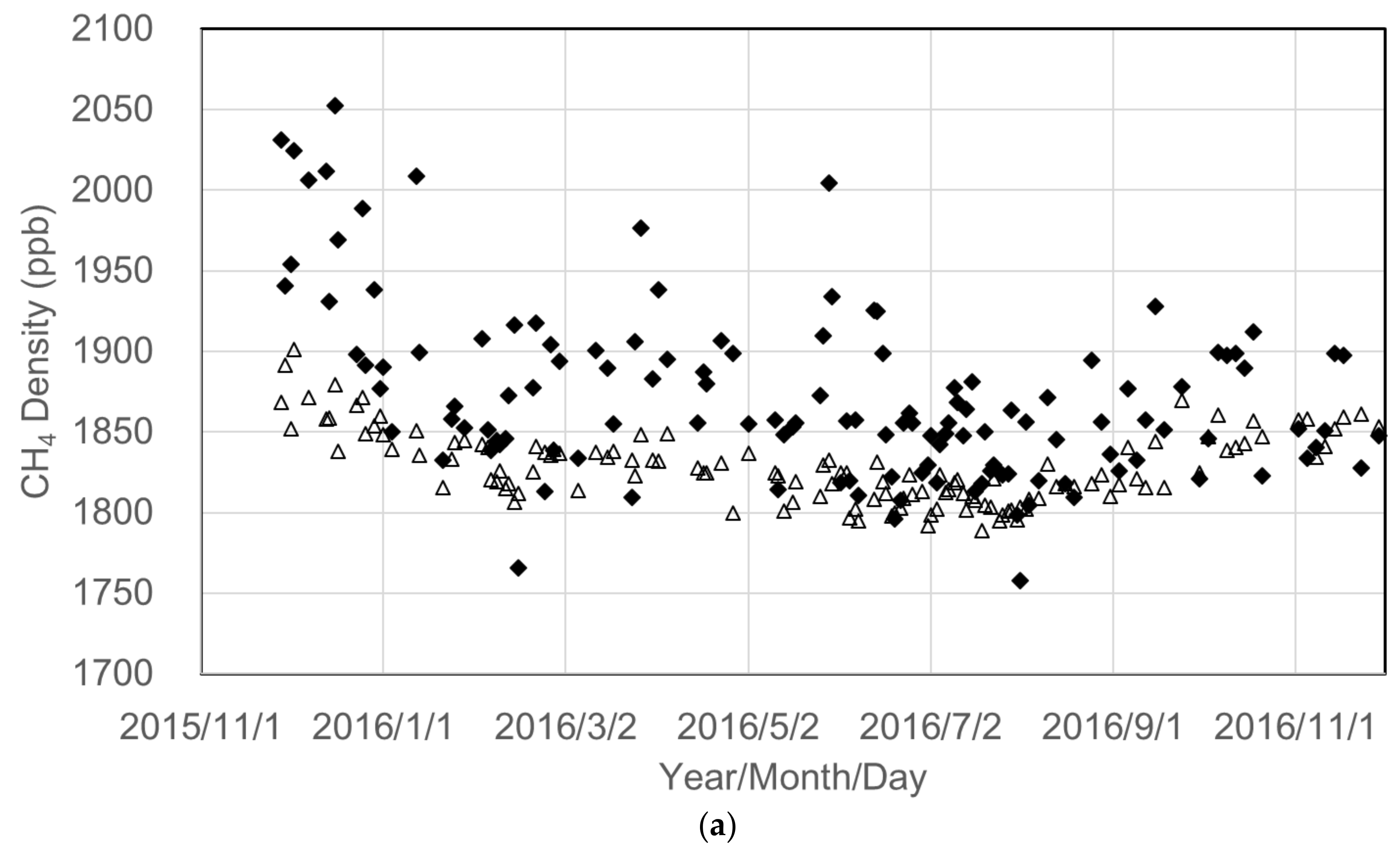
Figure 2a,b shows observed XCH4 and XCH4 (LT) and their DFS in retrieval. The LT data showed enhancement soon after the blowout event in 2015, which is much clearer than total column data. DFS values close to 1 demonstrate information content in the observed XCH4 (LT). Figure 3 shows the retrieved XCH4 (LT) and XCH4 (UT) at Aliso Canyon-S. The UT data did not indicate effect by the blowout event. Year-long data for both XCH4 (LT) and XCH4 (UT) showed decreases in summer, whereas, in the other seasons, the data largely fluctuated. Figure 3 shows XCH4(UT) data that are higher than those of XCH4 (LT). The possible cause is an inflow from other CH4 emission sources. There are several CH4 emission sources such as oil fields and dairy farms in California. We selected pairs of successfully retrieved data at Simi Valley as a reference to XCH4 (LT) at Aliso Canyon-S under clear-sky conditions. The detailed processes of background subtraction, normalization, and filtering are described in the Appendix A. Figure A1 shows the XCH4 (LT) enhancement from Simi Valley at: (a) Aliso Canyon-S; and (b) Aliso Canyon-N and Burbank after background subtraction. Figure A2 shows a reduction in the positive bias after normalization. Figure A3 shows the XCH4(LT)/XCO2(LT) ratio and the WRF wind direction at the leak point during GOSAT overpass for filtering. XCH4 (LT) data for both Simi Valley and Aliso Canyon-N/-S were possibly influenced by pollution inflow from the greater Los Angeles area. The measured XCH4 (LT) at these locations varied significantly, depending on wind conditions, resulting in large fluctuations. We assumed that: (1) urban pollution caused both CH4 and CO2 enhancements; (2) inflow to the reference point of Simi Valley and to Aliso Canyon had the same CH4 to CO2 ratios; and (3) no CO2 was emitted at the gas leak point on the hills of Aliso Canyon. XCH4 (LT) normalized by the retrieved XCO2 (LT) should remove the inflow portion inside the footprint.
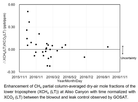
As illustrated in Figure 1b, the leak point was located at the edge of Aliso Canyon-N and outside of Aliso Canyon-S. The CH4 plume should not have entered the GOSAT footprint from any direction between 90° (east) and 315°. We rejected the data not meeting this criterion, based on Weather Research and Forecasting (WRF) model calculations [37]. We used simulated wind direction at the location of the leak point (34.31°N, 118.56°W), height of 906.9 hPa, and time of 20:50 UTC. As a result, large fluctuations in data were removed. The selected data showed a large enhancement in November (just after the blowout), followed by a clear decrease. The outliers above the uncertainty level of 0.056 ppb/ppm of △XCH4(LT)/XCO2(LT) were mostly removed, as shown in Figure 4. The flat topography of Aliso Canyon-S allowed for more accurate monitoring capability in detecting the blowout and confirming blocking of the leak. Figure 4 presents some data that have negative values larger than the uncertainty level, probably due to CH4 inflow, which is not correlated with CO2 enhancement. Simi Valley is not an ideal upwind reference.
4. Reducing Uncertainties in the Local Flux Estimation
There were four major causes of uncertainty in the case study for estimating the local flux from a point source using Equation (1): retrieval of XCH4 (LT), V, Ls, and background removal.
(a) Satellite remote sensing has common retrieval errors in forward calculation, in addition to random instrument noise and radiometric calibration errors. Multiple scattering by aerosols and clouds, bidirectional reflection on Earth’s surface, uncertainties in line parameters, and the solar model cause both bias and random errors. It is difficult to significantly reduce the current XCH4 retrieval uncertainty of 13 ppb. The GOSAT IFOV is too large, compared to the areas of the Aliso Canyon CH4 gas blowout. By improving spatial resolution to the scale of the emissions area, differential XCH4 (LT) measurements can be significantly enhanced, possibly enabling more accurate estimates of local CH4 emission.
(b) The number of sites where wind speed and direction are monitored regularly is limited. The data were available only at the Burbank Airport, which is 22 km away from the emissions source. In addition, their vertical profiles were not measured. Thus, we instead have to use a simulation such as the WRF model with large uncertainties. We need more validation data for the wind speed simulation in the boundary layer.
(c) In Aliso Canyon, the wind direction during the GOSAT overpass varied each day. The point of leakage was decentered for Aliso Canyon-N and outside the footprint for Aliso Canyon-S. Without accurate wind direction information, the flux cannot be estimated. Targeting the center of the emissions point can cover a plume in any wind direction. The present single-pixel GOSAT with its two-axis pointing system limits the number of observation points. Multi-pixel data will help in inferring the wind direction and in selecting proper reference points upwind for each flux estimate.
(d) A proper upwind reference closer to the emissions source assumed as a background can remove CH4 contamination from the surrounding area. Imaging capability and a smaller footprint with a flat topography would provide a more accurate background level than the current method using Simi Valley data. For example, XCH4 acquired by TROMOMI may be useful for this purpose [38]. A more robust algorithm for topography is also needed.
TANSO-FTS was designed to demonstrate accurate remote sensing from space with marginal spectral resolution using a single-pixel detector. FTS needs mechanical scan time to acquire the interferogram and the spectral resolution becomes worse when the off-axis angle becomes larger. Conventional space borne FTSs use near-optical axis areas: 1, 2 × 2, and 3 × 3 pixels for GOSAT, IASI, and CrIS, respectively. A grating spectrometer with a two-dimensional detector can acquire multiple pixel data in the CT direction within an electrical integration time, which is much shorter than the mechanical scan time of the GOSAT FTS. We can allocate spectral information in one dimension and CT electrical scan for the other dimension. Aberration-corrected grating technology can widen the CT field of view. With satellite motion, we can acquire image data that have at least 1000 times more sampling points than the existing GOSAT. To achieve this, we propose an imaging capability with a 1 km2 spatial resolution to monitor plume orientation and simultaneous measurement of short-lived species to estimate the wind speed and direction [39].
5. Conclusions
In this paper, we present a case study on CH4 emissions from a natural gas leak at Aliso Canyon using target observations with a pointing mechanism. We used the time-series of the partial column-averaged dry-air mole fractions of the lower troposphere, XCH4 (LT), retrieved by simultaneous use of reflected solar light and thermal emission. Frequent and long-term satellite observations, with appropriate background references, can detect CH4 enhancements from local-point emission sources and even capture total emissions. XCH4 (LT) minimizes the effects of inflow of CH4 in the UT and the stratosphere. The CH4 blowout event at Aliso Canyon was clearly seen in the temporal changes in XCH4 (LT). Normalization with XCO2 (LT) reduced the effects of CH4 inflow to the target areas. Geometric mismatch between the emission point and the center of the GOSAT footprint needed screening using the WRF wind direction data. However, the large footprint made it difficult to enhance XCH4 (LT) further with more flat topography and estimate the flux variation quantitatively. Imaging capability and a higher spatial resolution with a two-dimensional multi-pixel detector may reduce uncertainties in the local flux estimation from point sources.
Author Contributions
A.K. contributed to satellite operation, data analyses, and preparation of the manuscript. N.K. and F.K. are responsible for partial-column density retrieval and WRF calculation, respectively. H.S., K.S., and Y.K. selected target observation points and reviewed the data analysis. All authors have read and agreed to the published version of the manuscript.
Funding
This research received no external funding.
Acknowledgments
The authors thank Kenji Kowata of the Remote Sensing Technology Center of Japan and Emma Yates and Laura Iraci of NASA Ames research center. The authors also wish to thank the GOSAT operation team, RemoTeC team, and ACOS team. The level 1B radiance spectra data are available at GDAS. The GOSAT XCH4 data obtained in the target mode at the selected sites are available at http://www.eorc.jaxa.jp/GOSAT/CO2_monitor/index.html. European Commission: Emission Database for Global Atmospheric Research (EDGAR), release version 4.2, Tech. rep., Joint Research Centre (JRC)/Netherlands Environmental Assessment Agency (PBL), is available at: http://edgar.jrc.ec.europa.eu.
Conflicts of Interest
The authors declare no conflict of interest.
Appendix A. Background Subtraction, Normalization, and Filtering Processes
Appendix A.1. Background Subtraction Using Reference Point Data
Assuming the LT inflow is locally spatially constant, Equation (A1) calculates the enhancement from the point source using nearby reference data as follows:
where XCH4 (LT)s and XCH4 (LT)r are XCH4 (LT) over the source and reference points measured by GOSAT within the same orbit path, respectively.
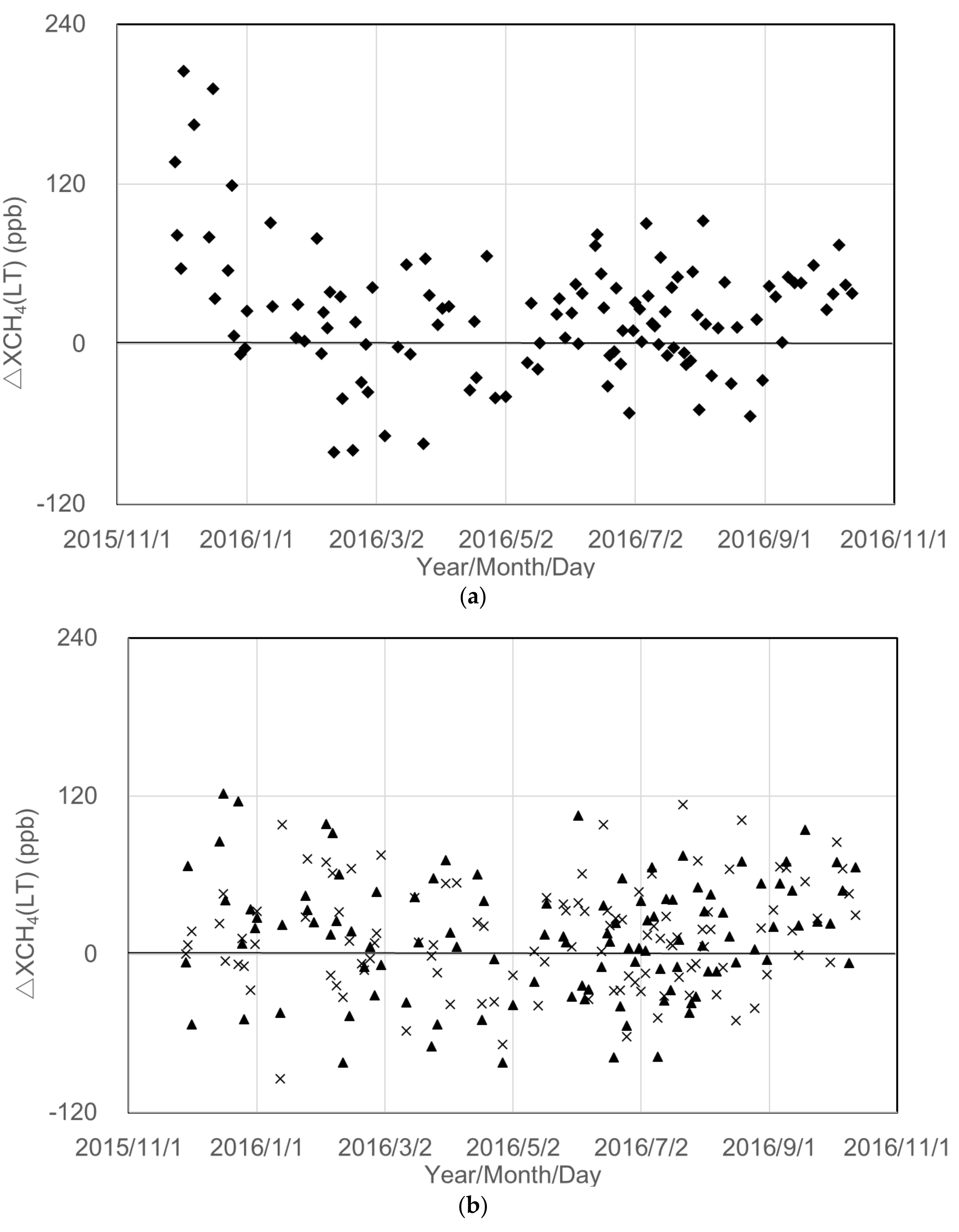
Figure A1 shows the XCH4 (LT) enhancement from Simi Valley at: (a) Aliso Canyon-S; and (b) Aliso Canyon-N and Burbank. Both Aliso Canyon-N and Aliso Canyon-S show enhancement in November and December 2015, and decrease with time in 2016. The enhancement in Burbank is less clear. Individual values show fluctuation and sometimes have negative values. Simi Valley, as a reference, is located close to the blowout point, but also close to urban areas. This is because the amount of inflow at Simi Valley was not the same for all the sites.
Figure A1.
Time trend of successfully retrieved data: (a) XCH4 (LT) enhancement from Simi Valley data of Aliso Canyon-S (diamonds); and (b) the same as (a) except for Aliso Canyon-N (triangles) and Burbank (crosses).
Figure A1.
Time trend of successfully retrieved data: (a) XCH4 (LT) enhancement from Simi Valley data of Aliso Canyon-S (diamonds); and (b) the same as (a) except for Aliso Canyon-N (triangles) and Burbank (crosses).

Appendix A.2. Normalization Process
As there are other CH4 and large CO2 emission sources in Southern California, we introduced the XCH4(LT)/XCO2(LT) ratio to reduce contamination by temporal inflow, which is not equal to the source and reference. Assuming the common virtual background for source and sink, the enhancement trend of Aliso Canyon can be monitored as presented in Equation (A2).
The suffixes e, b, si, and ri denote enhancement by emissions from the source, background, and inflow at the source and reference points, respectively.
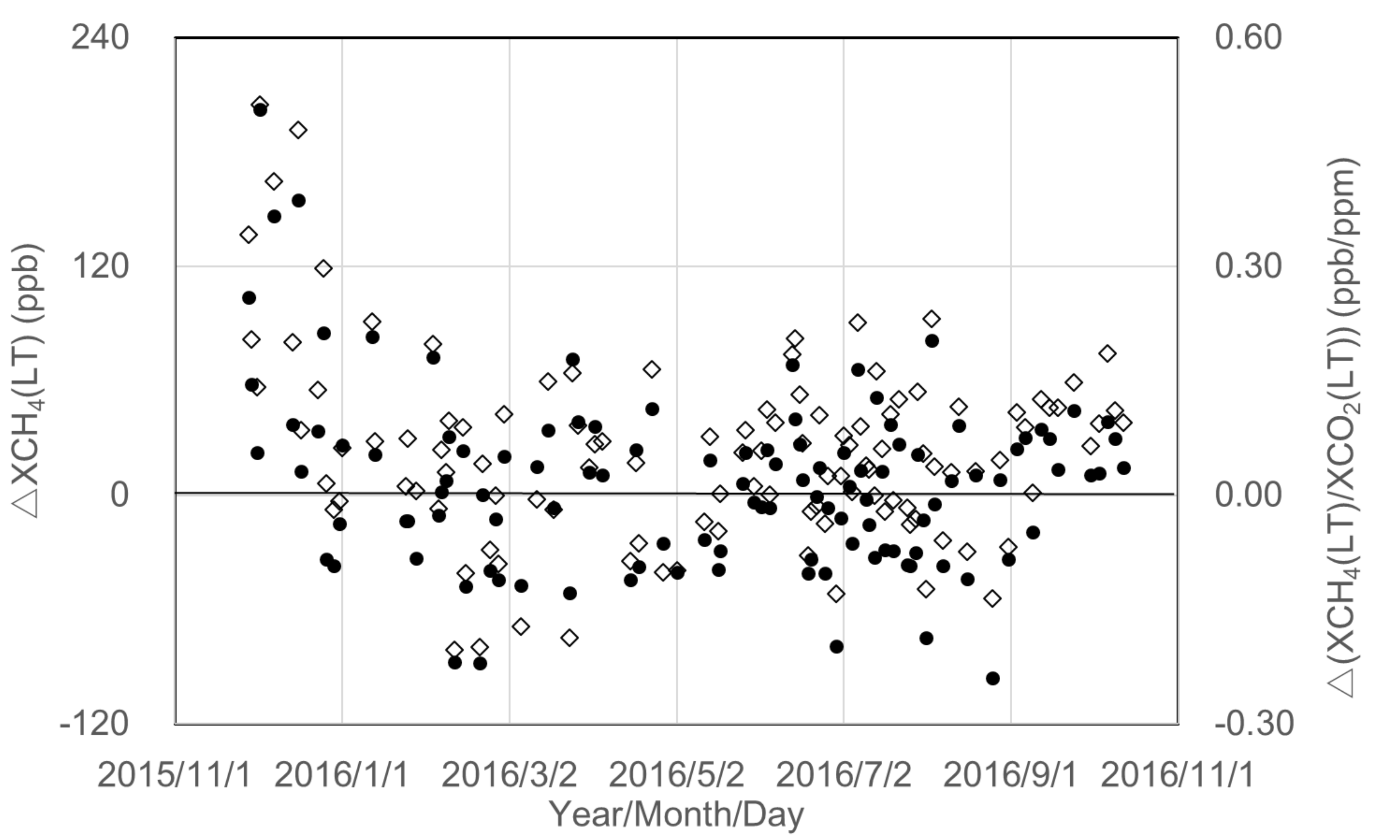
Aliso Canyon is surrounded by the Transverse Range and urban areas. There are both CO2 and CH4 emission sources in the urban areas; consequently, the inflow to Aliso Canyon has mixed contamination. Assuming that XCH4(LT)/XCO2(LT) of inflow to the source and reference from urban areas have common values, the above equation can extract enhancement from the CH4 point source. Figure A2 shows a reduction of 20 ppb in the positive bias in the case of background XCO2 (LT) of 400 ppm. Considering the uncertainty of 13 ppb in XCH4 (LT) and 2.1 ppm in XCO2 (LT) in the source and reference points, and assuming that both are random, the uncertainty level in enhancement is 0.056 ppb/ppm (Figure 4). This approach is effective for removing uncertainty due to the inflow and monitoring the trend, but we require wind information for quantitative discussion.
Figure A2.
XCH4 (LT) enhancement from Simi Valley data (diamonds) and for XCH4(LT)/XCO2(LT) (circles).
Figure A2.
XCH4 (LT) enhancement from Simi Valley data (diamonds) and for XCH4(LT)/XCO2(LT) (circles).

Appendix A.3. Filtering with Wind Direction
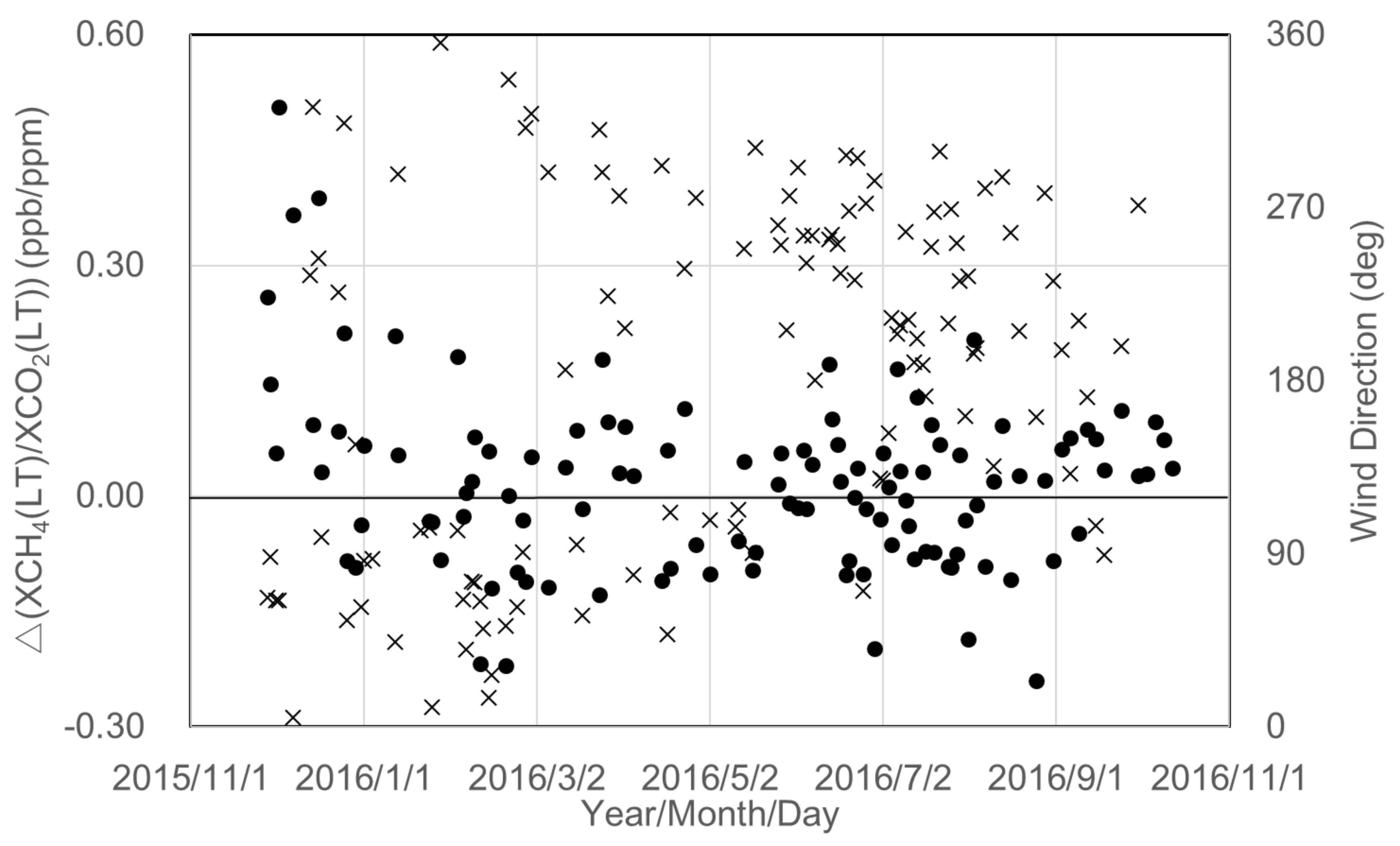
The sites where wind speed and direction are monitored regularly are limited. The data were available only at Burbank Airport, which is 22 km from the emissions source. Thus, we instead used the WRF model to simulate the actual atmospheric conditions. Figure A3 shows the XCH4(LT)/XCO2(LT) ratio and the WRF wind direction at the leak point (34.31°N, 118.56°W) during GOSAT overpass (20:50 UTC), at a height of 906.9 hPa. We filtered out data with a wind direction of East–South–Northwest (90–315°) using the WRF wind direction.
Figure A3.
XCH4(LT)/XCO2(LT) enhancement with time between the blowout and leak control (circles) as well as the WRF wind direction (crosses).
Figure A3.
XCH4(LT)/XCO2(LT) enhancement with time between the blowout and leak control (circles) as well as the WRF wind direction (crosses).
References
- Thompson, D.R.; Thorpe, A.K.; Frankenberg, C.; Green, R.O.; Duren, R.; Guanter, L.; Hollstein, A.; Middleton, E.; Ong, L.; Ungar, S. Space-based remote imaging spectroscopy of the Aliso Canyon CH4 superemitter. Geophys. Res. Lett. 2016, 43, 6571–6578. [Google Scholar] [CrossRef] [Green Version]
- Frankenberg, C.; Thorpe, A.K.; Thompson, D.R.; Hulley, G.; Kort, E.A.; Vance, N.; Borchardt, J.; Krings, T.; Gerilowski, K.; Sweeney, C.; et al. Airborne methane remote measurements reveal heavy-tail flux distribution in Four Corners region. Proc. Natl. Acad. Sci. USA 2016, 113, 9734–9739. [Google Scholar] [CrossRef] [Green Version]
- Duren, R.M.; Thorpe, A.K.; Foster, K.T.; Rafiq, T.; Hopkins, F.M.; Yadav, V.; Bue, B.D.; Thompson, D.R.; Conley, S.; Colombi, N.K.; et al. California’s methane super-emitters. Nature 2019, 575, 180–184. [Google Scholar] [CrossRef] [PubMed] [Green Version]
- Jacob, D.J.; Turner, A.J.; Maasakkers, J.D.; Sheng, J.; Sun, K.; Liu, X.; Chance, K.; Aben, I.; McKeever, J.; Frankenberg, C. Satellite observations of atmospheric methane and their value for quantifying methane emissions. Atmos. Chem. Phys. 2016, 16, 14371–14396. [Google Scholar] [CrossRef] [Green Version]
- Buchwitz, M.; de Beek, R.; Burrows, J.P.; Bovensmann, H.; Warneke, T.; Notholt, J.; Meirink, J.F.; Goede, A.P.H.; Bergamaschi, P.; Körner, S.; et al. Atmospheric methane and carbon dioxide from SCIAMACHY satellite data: Initial comparison with chemistry and transport models. Atmos. Chem. Phys. 2005, 5, 941–962. [Google Scholar] [CrossRef] [Green Version]
- Crisp, D.; Atlas, R.M.; Bréon, F.-M.; Brown, L.R.; Burrows, J.P.; Ciais, P.; Connor, B.J.; Doney, S.C.; Fung, I.Y.; Jacob, D.J.; et al. The Orbiting Carbon Observatory (OCO) mission. Adv. Space Res. 2004, 34, 700–709. [Google Scholar] [CrossRef] [Green Version]
- Yang, D.X.; Liu, Y.; Cai, Z.N.; Chen, X.; Yao, L.; Lu, D.R. First global carbon dioxide maps produced from TanSat measurements. Adv. Atmos. Sci. 2018, 35, 621–623. [Google Scholar] [CrossRef]
- Varon, D.J.; McKeever, J.; Jervis, D.; Maasakkers, J.D.; Pandey, S.; Houweling, I.; Aben, I.; Scarpelli, T.; Jacob, D.J. Satellite discovery of anomalously large methane point sources from oil/gas production. Geophys. Res. Lett. 2019, 46, 13507–13516. [Google Scholar] [CrossRef] [Green Version]
- Veefkind, J.; Aben, I.; McMullan, K.; Förster, H.; de Vries, J.; Otter, G.; Claas, J.; Eskes, H.; de Haan, J.; Kleipool, Q.; et al. TROPOMI on the ESA Sentinel-5 precursor: A GMES mission for global observations of the atmospheric composition for climate, air quality and ozone layer applications, the Sentinel missions—New opportunities for science. Remote Sens. Environ. 2012, 120, 70–83. [Google Scholar] [CrossRef]
- Eldering, A.; Kaki, S.; Crisp, D.; Gunson, M.R. The OCO-3 Mission; The American Geophysical Union Fall Meeting: San Francisco, CA, USA, 2013. [Google Scholar]
- Kuze, A.; Suto, H.; Nakajima, M.; Hamazaki, T. Thermal and near infrared sensor for carbon observation Fourier-transform spectrometer on the Greenhouse Gases Observing Satellite for greenhouse gases monitoring. Appl. Opt. 2009, 48, 6716–6733. [Google Scholar] [CrossRef]
- Kuze, A.; Suto, H.; Shiomi, K.; Kawakami, S.; Tanaka, M.; Ueda, Y.; Deguchi, A.; Yoshida, J.; Yamamoto, Y.; Kataoka, F.; et al. Update on GOSAT TANSO-FTS performance, operations, and data products after more than 6 years in space. Atmos. Meas. Tech. 2016, 9, 2445–2461. [Google Scholar] [CrossRef] [Green Version]
- Maddy, E.S.; Barnet, C.D.; Goldberg, M.; Sweeney, C.; Liu, X. CO2 retrievals from the Atmospheric Infrared Sounder: Methodology and validation. J. Geophys. Res. 2008, 113, D11301. [Google Scholar] [CrossRef] [Green Version]
- Beer, R.; Glavich, T.A.; Rider, D.M. Tropospheric emission spectrometer for the Earth Observing System’s Aura Satellite. Appl. Opt. 2001, 40, 2356–2367. [Google Scholar] [CrossRef] [PubMed]
- Clerbaux, C.; Boynard, A.; Clarisse, L.; George, M.; Hadji-Lazaro, J.; Herbin, H.; Hurtmans, D.; Pommier, M.; Razavi, A.; Turquety, S.; et al. Monitoring of atmospheric composition using the thermal infrared IASI/MetOp sounder. Atmos. Chem. Phys. 2009, 9, 6041–6054. [Google Scholar] [CrossRef] [Green Version]
- Tobin, D.; Tobin, D.; Revercomb, H.; Knuteson, R.; Taylor, J.; Best, F.; Borg, L.; DeSlover, D.; Martin, G.; Buijs, H.; et al. Suomi-NPP CrIS radiometric calibration uncertainty. J. Geophys. Res. Atmos. 2013, 118, 10589–10600. [Google Scholar] [CrossRef]
- Turner, A.J.; Jacob, D.J.; Wecht, K.J.; Maasakkers, J.D.; Biraud, S.C.; Boesch, H.; Bowman, K.W.; Deutscher, N.M.; Dubey, M.K.T.; Griffith, D.W.; et al. Estimating global and North American methane emissions with high spatial resolution using GOSAT satellite data. Atmos. Chem. Phys. 2015, 15, 7049–7069. [Google Scholar] [CrossRef] [Green Version]
- Sheng, J.-X.; Jacob, D.J.; Turner, A.J.; Maasakkers, J.D.; Benmergui, J.; Bloom, A.A.; Arndt, C.; Gautam, R.; Zavala-Araiza, D.; Boesch, H.; et al. 2010–2016 methane trends over Canada, the United States, and Mexico observed by the GOSAT satellite: Contributions from different source sectors. Atmos. Chem. Phys. 2018, 18, 12257–12267. [Google Scholar] [CrossRef] [Green Version]
- Wunch, D.; Toon, G.C.; Blavier, J.-F.L.; Washenfelder, R.A.; Notholt, J.; Connor, B.J.; Griffith, D.W.T.; Sherlock, V.; Wennberg, P.O. The Total Carbon Column Observing Network. Philos. Trans. R. Soc. A 2011, 369, 2087–2112. [Google Scholar] [CrossRef] [Green Version]
- Butz, A.; Guerlet, S.; Hasekamp, O.; Schepers, D.; Galli, A.; Aben, I.; Frankenberg, C.; Hartmann, J.-M.; Tran, H.; Kuze, A.; et al. Toward accurate CO2 and CH4 observations from GOSAT. Geophys. Res. Lett. 2011, 38, L14812. [Google Scholar] [CrossRef] [Green Version]
- Guerlet, S.; Butz, A.; Schepers, D.; Basu, S.; Hasekamp, O.P.; Kuze, A.; Yokota, T.; Blavier, J.-F.; Deutscher, N.M.; Griffith, D.W.T.; et al. Impact of aerosol and thin cirrus on retrieving and validating XCO2 from GOSAT shortwave infrared measurements. J. Geophys. Res. Atmos. 2013, 118, 4887–4905. [Google Scholar] [CrossRef] [Green Version]
- Schepers, D.; Guerlet, S.; Butz, A.; Landgraf, J.; Frankenberg, C.; Hasekamp, O.; Blavier, J.F.; Deutscher, N.M.; Griffith, D.W.T.; Hase, F.; et al. Methane retrievals from Greenhouse Gases Observing Satellite (GOSAT) shortwave infrared measurements: Performance comparison of proxy and physics retrieval algorithms. J. Geophys. Res. 2012, 117, D10307. [Google Scholar] [CrossRef] [Green Version]
- Crisp, D.; Fischer, B.M.; O’Dell, C.; Frankenberg, C.; Basilio, R.; Bösch, H.; Brown, L.R.; Castano, R.; Connor, B.; Deutscher, N.M.; et al. The ACOS XCO2 retrieval algorithm, Part II: Global XCO2 data characterization. Atmos. Meas. Tech. 2012, 5, 1–21. [Google Scholar] [CrossRef]
- Yoshida, Y.; Kikuchi, N.; Morino, I.; Uchino, O.; Oshchepkov, S.; Bril, A.; Saeki, T.; Schutgens, N.; Toon, G.C.; Wunch, D.M.; et al. Improvement of the retrieval algorithm for GOSAT SWIR XCO2 and XCH4 and their validation using TCCON data. Atmos. Meas. Tech. 2013, 6, 1533–1547. [Google Scholar] [CrossRef]
- Parker, R.; Boesch, H.; Cogan, A.; Fraser, A.; Feng, L.; Palmer, P.I.; Messerschmidt, J.; Deutscher, N.; Griffith, D.W.T.; Notholt, J.; et al. Methane observations from the Greenhouse Gases Observing SATellite: Comparison to ground–based TCCON data and model calculations. Geophys. Res. Lett. 2011, 38, L15807. [Google Scholar] [CrossRef] [Green Version]
- Saitoh, N.; Kimoto, S.; Sugimura, R.; Imasu, R.; Kawakami, S.; Shiomi, K.; Kuze, A.; Machida, T.; Sawa, Y.; Matsueda, H. Algorithm update of the GOSAT/TANSO-FTS thermal infrared CO2 product (version 1) and validation of the UTLS CO2 data using CONTRAIL measurements. Atmos. Meas. Tech. 2016, 9, 2119–2134. [Google Scholar] [CrossRef] [Green Version]
- Kikuchi, N.; Yoshida, Y.; Uchino, O.; Morino, I.; Yokota, T. An advanced retrieval algorithm for greenhouse gases using polarization information measured by GOSAT TANSO-FTS SWIR I: Simulation study. J. Geophys. Res. Atmos. 2016, 121. [Google Scholar] [CrossRef] [Green Version]
- Kikuchi, N.; Kuze, A.; Kataoka, F.; Shiomi, K.; Hashimoto, M.; Suto, H.; Knuteson, R.; Iraci, L.; Yates, E.; Gore, W.; et al. Three-Dimensional Distribution of Greenhouse Gas Concentrations over Megacities Observed by GOSAT; The American Geophysical Union Fall Meeting: San Francisco, CA, USA, 2017. [Google Scholar]
- Yates, E.L.; Lowenstein, M.; Iraci, L.T.; Tadic, J.; Sheffner, E.J.; Schiro, K.; Kuze, A. Carbon dioxide and methane at a desert site—A case study at Railroad Valley playa, Nevada, USA. MDPI Atmos. 2011, 2, 702–714. [Google Scholar] [CrossRef] [Green Version]
- Tadic, J.M.; Lowenstein, M.; Frankenberg, C.; Butz, A.; Roby, M.; Iraci, L.T.; Yates, E.L.; Gore, W.; Kuze, A. A comparison of in-situ aircraft measurements of carbon dioxide and methane to GOSAT data measured over Railroad Valley playa, Nevada, USA. IEEE Trans. Geosci. Remote Sens. 2014, 52, 7764–7774. [Google Scholar] [CrossRef]
- Tanaka, T.; Yates, E.; Iraci, L.; Johnson, M.S.; Gore, W.; Tadic, J.M.; Loewenstein, M.; Kuze, A.; Frankenberg, C.; Butz, A.; et al. Two year comparison of airborne measurements of CO2 and CH4 with GOSAT at Railroad Valley, Nevada. IEEE Trans. Geosci. Remote Sens. 2016, 54, 4367–4375. [Google Scholar] [CrossRef]
- Iraci, L.T.; Yates, E.L.; Parworth, C.; Kuze, A.; Kikuchi, N.; Kataoka, F.; Shiomi, K.; Suto, H.; Kulawik, S.S.; Basu, S. Vertical Profiles of Greenhouse Gases Collected over Land and Water in the Western US in Support of Partial Column Validation Efforts; A43R-3147; AGU Fall Meeting: San Francisco, CA, USA, 2019. [Google Scholar]
- Kataoka, F.; Knuteson, R.O.; Kuze, A.; Shiomi, K.; Suto, H.; Yoshida, J.; Kondo, S.; Saitoh, N. Calibration, Level 1 Processing and Radiometric Validation for TANSO-FTS TIR on GOSAT. IEEE Trans. Geosci. Remote Sens. 2019, 57, 3490–3500. [Google Scholar] [CrossRef]
- Bedford, B. Free flight time for projects in atmospheric sciences. EOS Earth Space Sci. News 2018, 99. [Google Scholar] [CrossRef]
- Conley, S.; Franco, G.; Faloona, I.; Blake, D.R.; Peischl, J.; Ryerson, T.B. Methane emissions from the 2015 Aliso Canyon blowout in Los Angeles, CA. Science 2016, 351, 1317–1320. [Google Scholar] [CrossRef] [PubMed] [Green Version]
- Weather Underground. Available online: https://www.wunderground.com/ (accessed on 30 December 2019).
- Skamarock, W.C.; Klemp, J.B.; Dudhia, J.; Gill, D.O.; Barker, D.M.; Duda, M.G.; Huang, X.-Y.; Wang, W.; Powers, J.G. A description of the advanced research WRF Version 3. NCAR Tech. Note NCAR/TN-475+STR 2008, 113. [Google Scholar] [CrossRef]
- Hu, H.; Landgraf, J.; Detmers, R.; Borsdorff, T.; Aan de Brugh, J.; Aben, I.; Butz, A.; Hasekamp, O. Toward global mapping of methane with TROPOMI: First results and intersatellite comparison to GOSAT. Geophys. Res. Lett. 2018, 45. [Google Scholar] [CrossRef]
- Kuze, A.; Suto, H. Imaging Spectrometer with an Agile Pointing System to Quantify Global and Regional Greenhouse Gas Fluxes and Monitor Localized Emission Sources. Trans. JSASS Aerosp. Tech. Jpn. 2018, 16, 147–151. [Google Scholar] [CrossRef]
Figure 1.
(a) Aliso Canyon location; and (b) geometric relationship between the leak point and the Greenhouse gases Observing SATellite (GOSAT) footprints (circles) in Simi Valley (dashed line), Aliso Canyon-N (dotted line), Aliso Canyon-S (bold line), and Burbank (dash-dotted line).
Figure 1.
(a) Aliso Canyon location; and (b) geometric relationship between the leak point and the Greenhouse gases Observing SATellite (GOSAT) footprints (circles) in Simi Valley (dashed line), Aliso Canyon-N (dotted line), Aliso Canyon-S (bold line), and Burbank (dash-dotted line).
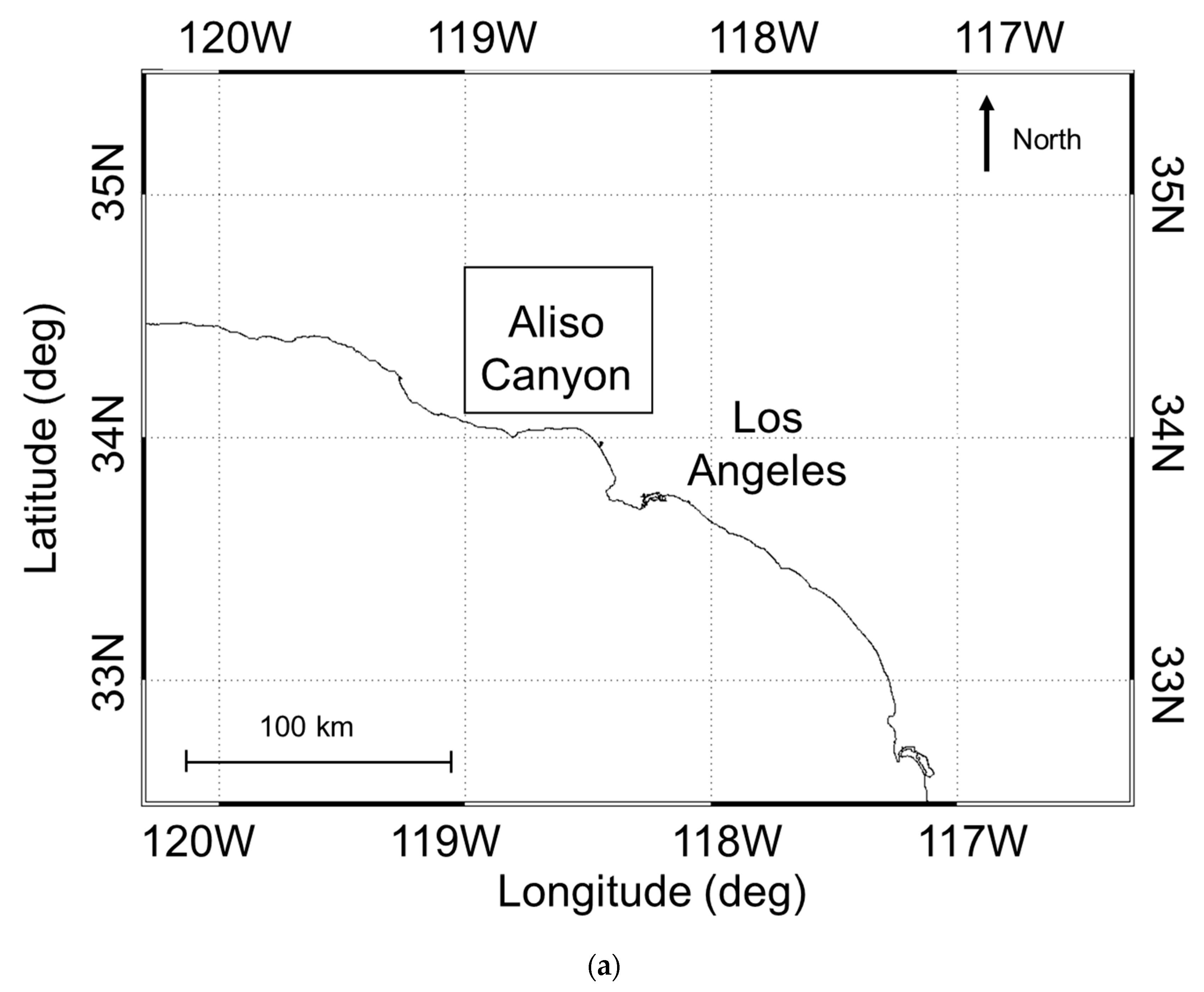
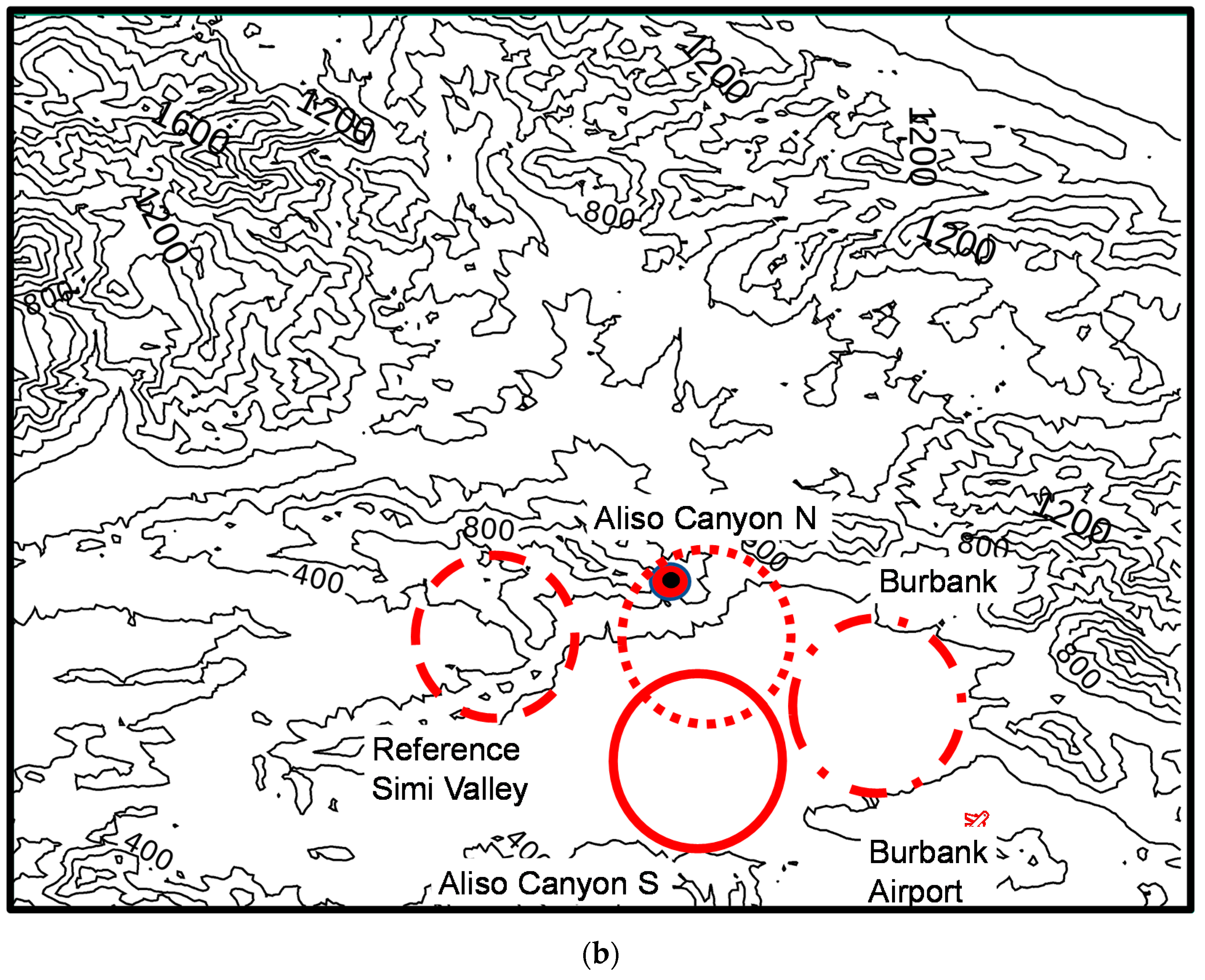
Figure 2.
(a) CH4 total partial column-averaged dry-air mole fractions (XCH4) (triangles) and the lower troposphere (XCH4 (LT)) (diamonds) at Aliso Canyon-S; and (b) the same as (a) except for the typical degrees of freedom for the signal (DFS) in retrieval.
Figure 2.
(a) CH4 total partial column-averaged dry-air mole fractions (XCH4) (triangles) and the lower troposphere (XCH4 (LT)) (diamonds) at Aliso Canyon-S; and (b) the same as (a) except for the typical degrees of freedom for the signal (DFS) in retrieval.

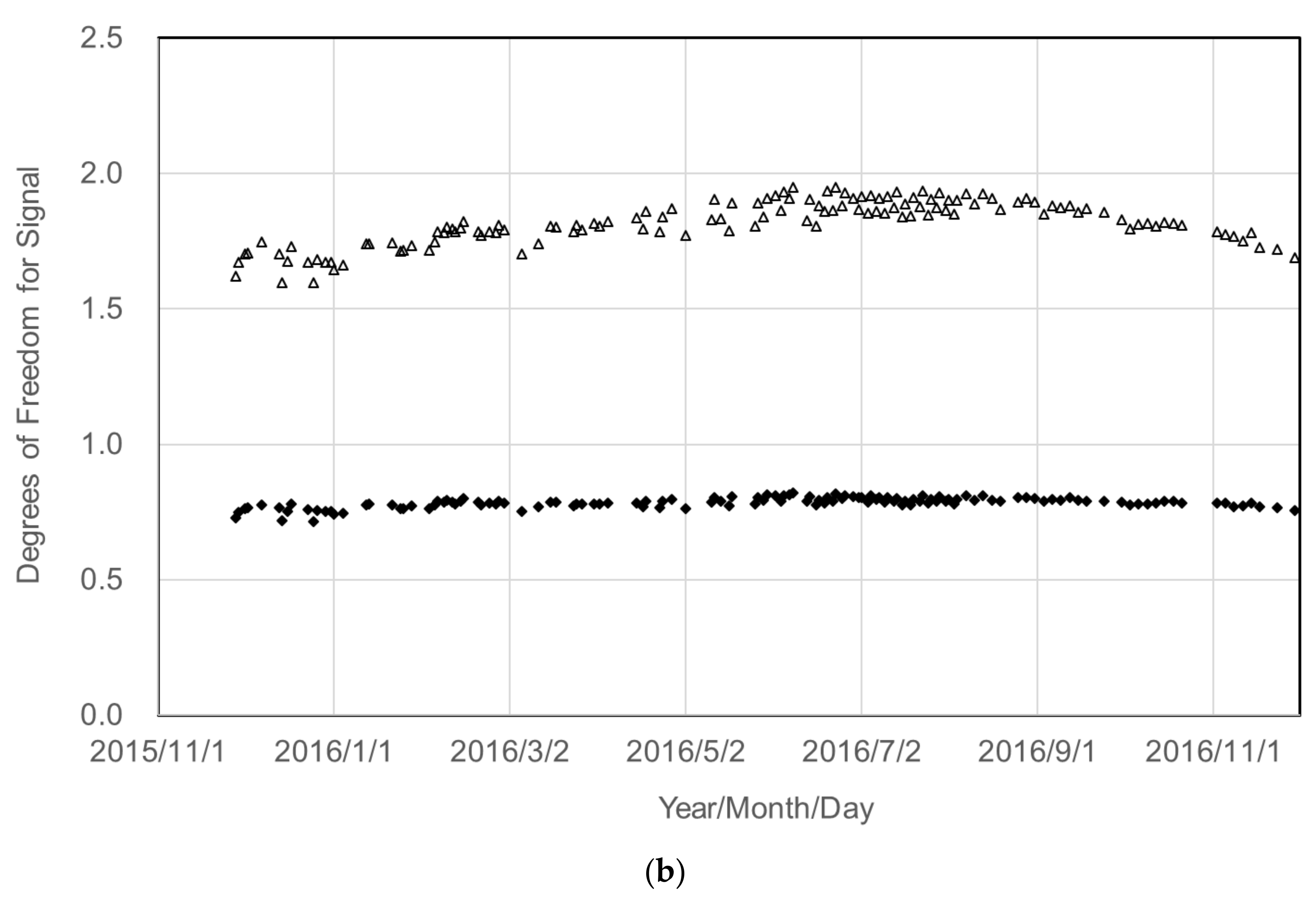
Figure 3.
CH4 partial column-averaged dry-air mole fractions of the lower troposphere (XCH4 (LT)) (diamonds) and the upper troposphere (XCH4 (UT)) (circles) at Aliso Canyon-S.
Figure 3.
CH4 partial column-averaged dry-air mole fractions of the lower troposphere (XCH4 (LT)) (diamonds) and the upper troposphere (XCH4 (UT)) (circles) at Aliso Canyon-S.

Figure 4.
XCH4 (LT) enhancements with time normalized with XCO2 (LT) between the blowout and leak control. Data with wind direction of East–South–Northwest at the leak point were filtered out.
Figure 4.
XCH4 (LT) enhancements with time normalized with XCO2 (LT) between the blowout and leak control. Data with wind direction of East–South–Northwest at the leak point were filtered out.


Table 1.
Nadir-viewing space-borne missions.
| Operation (Year) | Target | Reflected Solar Light | Thermal Emission | Pointing | Footprint | ||
|---|---|---|---|---|---|---|---|
| CO2 | CH4 | ||||||
| SCIAMACHY | 2002–2012 | ✓ | ✓ | ✓ | Entire surface | ||
| GOSAT | 2009–now | ✓ | ✓ | ✓ | ✓ | ✓ | Sparse |
| OCO-2 | 2014–now | ✓ | ✓ | Sparse | |||
| TanSAT | 2015–now | ✓ | ✓ | Sparse | |||
| GHGSat | 2016–now | ✓ | ✓ | ✓ | Sparse | ||
| TROPOMI | 2017–now | ✓ | ✓ | Entire surface | |||
| OCO-3 | 2019–now | ✓ | ✓ | ✓ | Sparse | ||
| AIRS | 2002–now | ✓ | ✓ | ✓ | Entire surface | ||
| TES | 2004–now | ✓ | ✓ | Sparse | |||
| IASI | 2006–now | ✓ | ✓ | Entire surface | |||
| CrIS | 2011–now | ✓ | ✓ | Entire surface | |||
Table 2.
Principal specifications of the GOSAT orbit and the TANSO-FTS instrument.
| Type of Orbit | Sun-Synchronized Sub-Recurrent Orbit | |
|---|---|---|
| Altitude of Orbit | 666 ± 0.6 km | |
| Local solar time | 13:00 ± 15 min | |
| Pointing mechanism | Cross track | ±35° |
| Along track: | ±20° | |
| Spectrometer | Type of interferometer | Double pendulum |
| Maximum optical path difference | ±2.5 cm (both sides) | |
| Aperture | 68 mm | |
| Scan speed (one way) | 4 s/Interferogram | |
| Interferogram acquisition | Both directions (forward and reverse scans) | |
| Instantaneous field of view | 15.8 mrad (10.5 km on the ground at nadir) | |
Table 3.
Specifications of spectral bands.
| Band 1 | Band 2 | Band 3 | Band 4 | |
|---|---|---|---|---|
| Spectral range (cm−1) | 12,900–13,200 | 5800–6400 | 4800–5200 | 700–1800 |
| Number of Linear polarization bands | 2 | 2 | 2 | N/A |
| Spectral resolution for P polarization (cm−1) * | 0.367 | 0.258 | 0.262 | N/A |
| Spectral resolution for S polarization (cm−1) * | 0.356 | 0.257 | 0.263 | N/A |
| Sampling interval (cm−1) | 0.2 | |||
| Detector | Si | InGaAs | InGaAs | PC-MCT |
* The spectral resolution is defined as full width at half maximum (FWHM) of the measured instrument line shape function (ILSF) before launch.
© 2020 by the authors. Licensee MDPI, Basel, Switzerland. This article is an open access article distributed under the terms and conditions of the Creative Commons Attribution (CC BY) license (http://creativecommons.org/licenses/by/4.0/).
Share and Cite
MDPI and ACS Style
Kuze, A.; Kikuchi, N.; Kataoka, F.; Suto, H.; Shiomi, K.; Kondo, Y. Detection of Methane Emission from a Local Source Using GOSAT Target Observations. Remote Sens. 2020, 12, 267. https://doi.org/10.3390/rs12020267
AMA Style
Kuze A, Kikuchi N, Kataoka F, Suto H, Shiomi K, Kondo Y. Detection of Methane Emission from a Local Source Using GOSAT Target Observations. Remote Sensing. 2020; 12(2):267. https://doi.org/10.3390/rs12020267
Chicago/Turabian StyleKuze, Akihiko, Nobuhiro Kikuchi, Fumie Kataoka, Hiroshi Suto, Kei Shiomi, and Yutaka Kondo. 2020. "Detection of Methane Emission from a Local Source Using GOSAT Target Observations" Remote Sensing 12, no. 2: 267. https://doi.org/10.3390/rs12020267
Note that from the first issue of 2016, this journal uses article numbers instead of page numbers. See further details here.