Compact Polarimetry Response to Modeled Fast Sea Ice Thickness


1
Science and Technology Branch, Environment and Climate Change Canada, Government of Canada, Dorval, QC H9P 1J3, Canada
2
Science and Technology Branch, Environment and Climate Change Canada, Government of Canada, Downsview, ON M3H 5T4, Canada
*
Author to whom correspondence should be addressed.
Remote Sens. 2020, 12(19), 3240; https://doi.org/10.3390/rs12193240
Submission received: 1 September 2020
/
Revised: 1 October 2020
/
Accepted: 1 October 2020
/
Published: 5 October 2020
(This article belongs to the Special Issue RADARSAT Constellation Mission (RCM))
Abstract
:Compact Polarimetric (CP) Synthetic Aperture Radar (SAR) is expected to gain more and more ground for Earth observation applications in the coming years. This comes in light of the recently launched RADARSAT Constellation Mission (RCM), which uniquely provides CP SAR imagery in operational mode. In this study, we present observations about the sensitivity of CP SAR imagery to thickness of thermodynamically-grown fast sea ice during early ice growth (September–December 2017) in the Resolute Bay area, Canadian Central Arctic. Fast ice is most suitable to use for this preliminary study since it exhibits only thermodynamic growth in absence of ice mobility and deformation. Results reveal that ice thickness up to 30 cm can be retrieved using several CP parameters from the tested set. This ice thickness corresponds to the thickness of young ice. We found the surface scattering mechanism to be dominant during the early ice growth, exposing an increasing tendency up to 30 cm thickness with a correlation coefficient with the thickness equal to 0.86. The degree of polarization was found to be the parameter with the highest correlation up to 0.95. While thickness retrieval within the same range is also possible using parameters from Full Polarimetric (FP) SAR parameters as shown in previous studies, the advantage of using CP SAR mode is the much larger swath coverage, which is an operational requirement.
1. Introduction
The Compact Polarimetric (CP) Synthetic Aperture Radar (SAR) configuration is gaining increased attention, especially following the launch of the RADARSAT Constellation Mission (RCM) in June 2019. Owned and operated by the Government of Canada, the RCM consists of the evolution of the RADARSAT program, which started back in 1995 with the launch of the RADARSAT-1 satellite [1]. The RCM uniquely provides in operational mode the CP option by transmitting a right-circularly polarized radar signal and receiving two mutually coherent orthogonal (horizontal and vertical) linear polarizations [2]. The increased swath of CP SAR configuration compared to the limited swath from the Full- (or quad-) Polarimetric (FP) SAR mode is an advantage for operational applications. Another advantage is the enhanced radar target information compared to conventional single and dual SAR systems [3].
One of the fundamental operational SAR applications, which could benefit from the CP SAR configuration, is the sea ice monitoring. A few studies explored the potential of CP SAR imagery for this application. Most of these studies are based on simulated CP SAR data. In [4], the potential of CP SAR data for classification of First Year Ice (FYI), Multiyear Ice (MYI) and Open Water (OW) in the spring before the onset of ice melting was investigated. The study used a large set of CP parameters derived from simulated CP SAR imagery for low and medium RCM imaging modes. This was followed by a more comprehensive study in [5] where CP parameters were investigated for all-season classification of ice types. In [6], CP parameters derived from simulated CP SAR imagery of the high-resolution RCM imaging mode were analyzed for classification of FYI and MYI. In [7], it was shown that automated classification of sea ice types using CP parameters or reconstructed pseudo quad pol data provides improved classification results, compared to conventional dual polarized SAR imagery. The reconstruction strategy of pseudo quad information from simulated CP SAR imagery was also investigated in [8] for sea ice classification. In [9], the potential of CP SAR parameters extracted from simulated CP SAR imagery for estimation of the fraction of melt ponds in Arctic sea ice was demonstrated. A new CP ratio was proposed in [10] for the retrieval of undeformed FYI thickness.
Only a limited number of studies explored the potential of CP SAR configuration for sea ice monitoring using real CP SAR imagery. For instance, [11] compared a set of CP parameters extracted from Radar Imaging Satellite 1 (RISAT-1) CP SAR imagery with CP parameters extracted from simulated CP SAR imagery obtained using near collocated RADARSAT-2 FP SAR imagery over seasonal sea ice during the melt season. This study was the first to investigate the possible effect of the non-perfectly circular RISAT-1 signal on the discrimination between sea ice types. In another study [12], RISAT-1 CP SAR imagery was evaluated for its capability in seasonal sea ice observation over Northeastern Greenland during the melt season. Herein, a mutual information analysis was applied for the extraction of optimum CP parameters for sea ice classification [12].
The innovative aspect of this study lies in the fact that it is the first to present the sensitivity of a large set of CP parameters to modeled ice thickness for thermodynamically-grown fast sea ice. Such a study is important since it comes in light of the new RCM which has been designed to provide CP SAR imagery in operational mode, supporting operational SAR applications such as sea ice monitoring. Fast ice was selected because its thickness is mostly thermodynamically-grown with no mechanical growth attributed to deformation caused by ice mobility. This latter factor impedes the use of SAR for ice thickness retrieval. CP parameters are extracted from simulated CP SAR data using a stack of 62 RADARSAT-2 FP images, which were acquired over the Resolute Bay area in the Canadian Central Arctic during the fall of 2017.
We analyze the temporal evolution of the extracted parameters against modeled ice thickness estimated for fast sea ice in Resolute Bay and a neighboring nameless fjord, which we named Fjord X. The model is initiated with weather data from the Resolute Weather Station of Environment and Climate Change Canada (ECCC). A resident operator of the Upper Air Network of ECCC at Resolute Bay provided limited field observations about the ice development. In this study, we also calculate and briefly analyze the correlation between the CP parameters for possible information redundancy.
It is important to clarify that our study is not intended to be a conclusive analysis of the sensitivity of CP parameters to fast sea ice thickness during early ice growth, since such a study would require intensive field measurements with coincident real CP SAR imagery and possibly ground-based polarimetric scatterometer measurements. The study rather aims at highlighting observations on trends of evolution of selected CP parameters with ice thickness estimated from an empirical model most suitable for thin ice. Such a study helps in better understanding the impacts of climate change on ice phenology and ice thickness in the Arctic region. We think this study is timely since the RCM has become recently operational (end of December 2019).
2. Study Area and SAR Imagery
Two sea water bodies located in Cornwallis Island, Canadian Central Arctic, were selected for the study (Figure 1): Resolute Bay (RB) and a nameless fjord located northwest of RB which we call Fjord X (FX). As shown in Figure 1, FX differs from RB in its narrower entrance, which limits the interaction between the ice inside and outside the fjord. This is not the case for RB with its wider entrance to Resolute Passage, which makes the intrusion of sea ice from outside easier. The intrusion of sea ice from outside the bay disturbs the formation of the ice inside the bay. Therefore, one would expect a delay in the onset of uninterrupted thermodynamic freezing of RB, when compared to FX.
The Resolute Weather Station, located at about 4 km northwest of RB, provided hourly and daily-average weather information, including air temperature, wind speed and direction, and snow fall. The air temperature and wind information were used to calculate the thickness of thermodynamically-grown ice in the two sites. Our analysis was further supported through site observations recorded by a resident operator of the Upper Air Network of ECCC at RB.
Given that our study is partly dealing with thin ice during the early ice growth at the onset of the dark season then with thicker ice well into the season, in situ measurements of ice properties, such as thickness, salinity, and snow cover were not feasible. Moreover, since snow in the region is mostly drifted, its distribution and properties (e.g., depth, density, and metamorphism) are highly variable within short distances and time scales. This was confirmed by the resident operator of the Upper Air Network of ECCC.
A set of 62 RADARSAT-2 FP SAR images was acquired between 20 September 2017 and 28 December 2017 (the onset of early ice freezing until it matures) covering the study area shown in Figure 1. The acquired data from different imaging beam modes between FQ7W and FQ20W are shown in Table 1. This gives a maximum range of incidence angle difference equal to 14.2° from all acquisitions. In [13], the effect of this range from the same dataset on the calibrated backscatter was proven to be negligible.
3. Methodology
3.1. Ice Thickness Modeling
All thermodynamic ice thickness models depend on the Freezing Degree Days (FDD). This term is defined as the sum of the daily temperatures below the freezing point in a given number of days. For example, if the daily average air temperature above the sea is −2.8, −3.4, and −5.6 °C and the freezing temperature of sea water is −1.8 °C, then FDD = 1 + 1.6 + 3.8 = 6.4 °C. In the absence of field measurements, ice thickness in our study is estimated using a well-known established empirical model [14] which accounts for the sensible heat loss when the ice is thin and the difference between its surface temperature and air temperature is large. Neglecting this factor causes underestimation of the thickness. The error is more severe at smaller FDD and almost abates at FDD = 50. Herein, ice thickness () of thermodynamically-grown sea ice is estimated using the following equation
where is the thermal conductivity (2.1 J.m−1s−1K−1), is the density (900 kg.m−3), is the latent heat of fusion (292 kJ.kg−1) and is a coefficient which accounts for the sensible heat flux from the ice surface to the air and depends on the wind speed. Based on [14], = 20 W.m−2 °C−1 was selected. This value suits the nominal range of wind speed in the present study area (between 10 and 30 km/h), and was successfully used in [13]. By investigating the sensitivity of to the selection of , we found higher sensitivity at small . For example, a change of ±2 of from its selected value of 20 would result in an 8% change of at 2 cm ice thickness, 2.5% when the thickness reaches 30 cm, and less than 1% when the thickness exceeds 1 m. Nevertheless, since the wind speed varies continuously over the ice cover, an average value of had to be selected. The above model comes with uncertainty since it implies some assumptions about the ice, such as the snow-free ice surface. As mentioned before, accurate and continuous snow data (depth, density, wetness, and metamorphism) was not feasible to obtain in the present study due to the dark season and the difficulty of monitoring the snow at the fine resolution of SAR over the large area of the selected bay and fjord. The snow is mostly drifted in this area, as confirmed by the resident operator of the Upper Air Network of ECCC at Resolute Bay, causing frequent changes in depth and compactness at short temporal and spatial scales. More information about the uncertainty of the used model for ice thickness estimation is presented in [14]. It is worth mentioning that C-band SAR signal penetrates dry snow up to 2 m [15]. However, the backscatter data in the present study must have originated from either a snow-free ice surface or the base of the snow layer when brine is wicked up during the ice thickness growth.
3.2. Ice Salinity Modeling
The ice bulk salinity (), defined as the average salinity over the entire thickness of the ice sheet, can be estimated in terms of ice thickness using a commonly-used empirical model as follow [16]
where h is the ice thickness. In (2), the bulk salinity is estimated in parts per thousand (‰). This empirical model suggests a linear relationship between ice bulk salinity and ice thickness. According to this equation, the at the onset of ice formation is 14.24‰. This is a reasonable value for fast ice, which usually pursues a columnar ice crystalline structure. If ice is initially formed under turbulent water conditions, frazil ice crystals are usually encountered, which brings to higher values [17,18]. The value of the constants in Equation (2) changes when the ice thickness exceeds 40 cm.
3.3. CP SAR Simulation
Although real CP SAR data are currently available from RCM, which is presently passing its early operational phase, our study is based on simulated CP SAR data. This is because the RCM was declared operational at the end of December 2019 after the end of the required period for such a study. Furthermore, requests for real-time SAR data acquisition (specifying period, location, SAR mode, etc.) should be submitted ahead of the acquisition period. Using simulated CP data is a necessary step to show the potential of the application, hence assisting in developing a data acquisition request. The Canada Center for Mapping and Earth Observation (CCMEO) has developed an in-house simulator for the simulation of CP SAR data. The simulator accepts as input RADARSAT-2 FP SAR imagery. The RADARSAT-2 16-bit complex HH, HV, VH, and VV products are converted to 32-bit floating complex by applying the provided calibration coefficients. Then, assuming a compact SAR configuration transmitting a right circular signal and coherently receiving linear (horizontal and vertical), the complex CP products RH (right circular transmission and linear horizontal receive) and RV (right circular transmission and linear vertical receive) can be given as follows [19]:
The complex RH and RV are converted to Stokes vector, which is then speckle filtered and used for the extraction of a total of 22 CP parameters shown in Table 2. Detailed information about the calculation of these parameters is presented in [4]. The derived CP parameters are sampled at the location of RB and FX for each of the 62 acquisitions (red polygons in Figure 1). It is worth mentioning that the sampling of RB and FX is performed in the flat surface of the fast ice. We avoid fast ice edges which might be affected by ocean waves or mobile ice. The number of selected pixels for RB is 35009, while for FX is 53373. Thus, we obtained a time series of the mean values of each CP parameter at the location of each site.
4. Backscattering Variation in Early Ice Growth
This section includes a brief account on the variation of the linear backscatter coefficients—namely and —during the early growth phase of sea ice, up to approximately 30 cm thick. These parameters are not used in this study. The information was obtained from established results in published studies. It serves as a point of reference to evaluate the performances of the selected CP parameters in this study to retrieve thin ice thickness. Previous studies show that and increase as sea ice thickness increases during the early growth phase. In a laboratory experiment, [24] found that co-polarization backscatter measured in C-band from sea ice increased with thickness and reached a peak at 30 cm before declining to reach a minimum at 150 cm thick. Data were obtained from artificial sea ice grown in an outdoor tank and confirmed using observations from a real aperture radar onboard of Cosmos satellite. Another study [25] reported a gradual increase in starting from the phase of grease/frazil ice (a few millimeters) throughout the phase of light nilas (an ice sheet of matte surface of thickness up to 10 cm). The data were obtained from scatterometer measurements in a thin ice field in the Arctic. In a different laboratory experiment to relate C-band polarimetric measurements to ice physical properties and assess the inversion of ice thickness [26], the authors observed an increase in co-polarization backscatter between 6 to 10 dB as ice grew from 3.0 to 11.2 cm in thickness. The data were obtained from a FP airborne SAR. This study suggested that the large enhancement of backscattering during the early sea ice growth period could be attributed to the increased brine pockets/channels during this active period of desalination. Using ENVISAT ASAR data, [27] shows maps of increasing by about 10 dB, measured from thin sea ice in the Ross ice shelf polynya, Antarctica, as ice thickness increased from a few centimeters to near 20 cm. In principle, the interconnection between the dense brine pockets/drainage channels might have increased scattering within the subsurface area. On the other hand, the desalination causes a decrease in the dielectric constant, which means less surface scattering. A full explanation of the backscattering increase with thickness from saline ice during its early formation phase has not been resolved. The above information is important as many of the CP parameters presented in the next section behave in the same manner as the linear backscattering coefficients during the early ice thickness range (0–30 cm).
5. Results
5.1. Evolution of Air Temperature, Ice Thickness, and Bulk Salinity
The evolution of air temperature (Figure 2a) revealed a continuous decreasing trend up to the middle of November. Between the middle and the end of November, air temperature began an increasing trend, which reached a daily average air temperature close to −4 °C. Then, the temperature resumed its winter decreasing trend. Figure 2b shows that the onset of uninterrupted ice thickness growth in FX started on 16 September, a few days earlier than the start in RB on 27 September. This is expected given the narrow entrance of FX which prevents the exchange of ice with the open sea. This exchange was allowed under the wind action between RB and the open sea, through its wide opening to Resolute Passage (Figure 1). As was reported by the resident ice operator at the Resolute Weather Station, prior to 27 September, the bay was partly filled with older ice imported from the passage, then the ice was cleared off in response to a strong wind on 26 September which varied between 30 and 63 km/h. Detailed information about the ice development at the experimental site before and after the onset of ice growth in both RB and FX can be found in [13].
Figure 2b also presents the evolution of the bulk salinity of sea ice in FX, which is slightly different than that in RB (not shown in Figure 2b). The salinity reveals a sharp decrease in the first 40 cm thickness, then the rate becomes milder for higher thickness. This is physically explained as brine drainage decreases at a lower rate as ice thickness increases [17,18]. The direct dependence of the thickness model and the indirect dependence of the salinity model on the FDD produce the continuous relations shown in Figure 2b. However, when the salinity and thickness are plotted against air temperature, new information emerges (Figure 3). Here, the data from each ice parameter are divided into two sets: one before 20 October and the second after 20 October. This date marks the ice thickness reaching 40 cm in both RS and FX. Before October 20, both parameters follow the linear trends shown by regression lines in Figure 3. This means that the increase in ice thickness during this period is associated with a trend of decrease in bulk salinity. After October 20 (i.e., when the ice becomes thicker than 40 cm), cold temperature still causes thickness increase, though at rates proportional to the increment of daily air temperature. On the other hand, brine drainage slows down, and salinity reaches a stable value between 6‰ and 8‰. Any change in air temperature in this case should affect brine volume and salinity through expansion and contraction of brine pockets and salt precipitation or melt within the pockets [17,18]. Two corollaries follow from the data in Figure 3. If radar parameters can be linked to the ice thickness during the initial ice growth phase (up to 30 cm thick), then they must be triggered by the sub-surface salinity or the bulk salinity. Secondly, if that turns out to be true, the rate of change of the bulk salinity during the same period can also be estimated. The absolute value cannot be estimated because we do not know the initial salinity trapped at the onset of freezing as this depends on the crystalline structure of the ice at that time, which is determined by the oceanic conditions—namely ice formation under turbulent (i.e., frazil ice) of quasi-steady surface (i.e., congealed ice).
5.2. CP Sensitivity to Ice Thickness
5.2.1. Backscattering Coefficients
The temporal evolution of the backscattering coefficients , , , and as a function of the modeled ice thickness is shown in Figure 4. Values of , , and reveal a linear increasing trend with ice thickness increase within a range up to 30 cm, which corresponds to the maximum thickness of young ice. After this thickness, the values decrease slightly before they stabilize after 50 cm thick around −20 dB for and , and −18 dB for . The aforementioned backscattering values from the smooth surface of the fast sea ice should be considered as a benchmark to convert the higher backscattering from rough or deformed ice surface in a drifted ice regime to estimate the degree of roughness or deformation. The behavior of , , and is identical to that from the two linear orthogonal co-polarized backscattering coefficients and as well as the total power from the quad pol mode of the same data set [13]. The stable value of both and is around −17 dB and the total power around −10 dB [13]. The backscattering coefficient achieves the highest correlation (0.84) with the first 30 cm of ice thickness. The lowest correlation (0.76) is given by . reveals only a tangible increasing trend during the first 30 cm of ice growth then stabilizes at a lower value of −25 dB. Since this parameter is highly correlated with the volume scattering mechanism [5], its slight increase at the onset of freezing might be an indication of the presence of volume scattering from the dendritic interface at the bottom when the ice is thin enough for the C-band to reach the interface, assuming no or transparent snow cover. In general, is not useful for ice thickness estimation because of its limited dynamic range.
5.2.2. Scattering Mechanisms
Variation of the three parameters that represent the scattering mechanisms (surface, volume, and double-bounce), obtained from the m-χ decomposition, against the ice thickness are presented in Figure 5. Figure 5a shows the sensitivity of surface scattering to ice thickness within the same range (up to 30 cm thick) shown by the backscattering coefficients. For ice thicker than 30 cm, the intensity of the surface scattering decreases slightly before it stabilizes around −20 dB once the thickness exceeds 50 cm. The typically smooth fast ice surface triggers a stable value of surface scattering. Here, surface scattering must have occurred from either a snow-free ice layer or the basal snow layer if it holds considerable brine volume. Within the 30 cm ice thickness, the linear trend line achieves a correlation of 0.86 (Figure 5a). As shown in Figure 5b, volume scattering reveals a limited increasing trend during the first 15 cm (although we did not have enough data points in the present set to establish a statistical significance of this observation). Here, the volume scattering from the first few points (thickness around 10 cm) is comparable to the surface scattering. This could be explained by the relatively large scattering portion of the signal from the dendritic ice–water interface, assuming a snow-free ice surface [13]. The stable value of volume scattering, encountered as ice exceeds 30 cm, is around −23 dB, which is slightly lower than the corresponding stable value of surface scattering (−20 dB). As expected, the double-bounce scattering is much lower (around −35 dB) and negligible; however, it mimics the same trend of increase then decrease within the first 20 cm of thickness (Figure 5c).
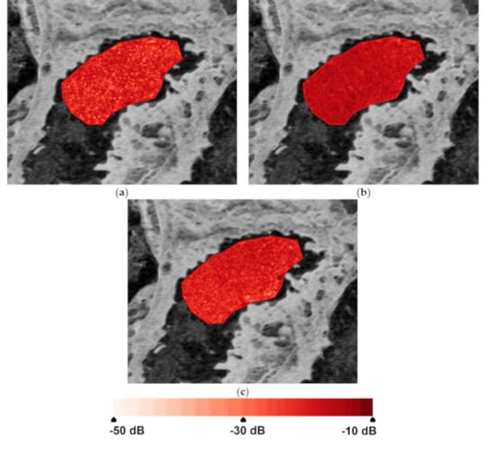
Our results indicate that surface scattering is the dominant scattering mechanism from a thermodynamically-grown fast sea ice. Therefore, we selected FX in Figure 6a–c to show the temporal differences of this mechanism as the ice grows. Figure 6a shows the intensity of the surface scattering mechanism for estimated ice thickness of 14.3 cm (27 September). This intensity reached its peak for ice thickness of 29.6 cm (≈30 cm) on 10 October, as shown in Figure 6b. The intensity of surface scattering slightly dropped before it stabilized for thickness exceeding 50 cm, as shown in Figure 6c (estimated thickness 122.1 cm on 25 December). It is worth noting that the scattering mechanisms from the m-δ decomposition provided results similar to those from the m-χ decomposition. Hence, we limit our presentation here to the m-χ decomposition results.
5.2.3. Stokes Vector
The Stokes vector consists of four elements: SV0 which is equal to the total average received power, SV1 which is equal to the power in the linear horizontal (SV1 > 0) or vertical (SV1 < 0) polarized components, SV2 which is equal to the power in the linearly polarized at tilt angle 45° (SV2 > 0) or tilt angle 135° (SV2 < 0) components, and SV3 which is equal to the average power received in left-circular (SV3 > 0) or right-circular (SV3 < 0) polarization [28].
Variations of the four elements of the Stokes vector with ice thickness are presented in Figure 7. While the four parameters exhibited remarkable variations until a 50 cm thickness, the linear increasing trend until a 30 cm thickness was clearer for SV0 and SV3. Between 30 and 50 cm, the values of SV0 and SV3 decreased, before relatively stabilizing beyond 50 cm ice thickness. The correlation coefficients from the regressed data of SV0 and SV3 are 0.79 and 0.87, respectively. The positive values of SV3 agree with the previously observed surface scattering mechanism which switches the right-circular incident signal to left-circular scattered signal. Beyond 50 cm thickness, SV1 exhibited a fairly constant value from both RB and XF around zero, indicating a power in linear horizontal or vertical close to zero. For the other three parameters, the variability in the stable zone beyond 50 cm ice thickness seems visually lower in the case of FX. This probably reflects the more stable conditions of the ice in FX as its interaction with the mobile ice from Resolute Passage is more limited due to its narrow opening to the passage.
5.2.4. Shannon Entropy
The Shannon entropy consists of two components: the intensity (SE_Int) and the polarimetric (SE_Pol). The SE_Int component is a scaled value of the total backscattering power SV0 [4], while the SE_Pol component depends on the Barakat degree of polarization [21]. The temporal evolution of the SE_Int (Figure 8a) and SE_Pol (Figure 8b) components with ice thickness reveals the same linear increasing trend up to 30 cm, similar to that observed from the above described parameters. After that thickness, the values of both components slightly dropped until they relatively stabilized at about 50 cm thick. It is worth noting the slight increase in the SE_Pol component between 85 and 95 cm ice thickness, which happened during the air temperature increase between the middle and the end of November. Therefore, it seems that this air temperature increase has raised the wetness of the snow cover which caused a rise in the polarization of the returned signal. Interestingly, the SE_Pol achieved a much higher correlation value (0.90), compared to the SE_Int (0.81), during the linear increasing trend (Figure 8).
5.2.5. Degree of Polarization, Conformity, and RH RV Correlation Coefficients
The evolution the degree of polarization (m), the conformity coefficient (μ), and the RH RV cross-correlation coefficient () with ice thickness are presented in Figure 9. The μ ranges between −1 to 1. Values of μ close to 1 pronounce the presence of the surface scattering mechanism, while for μ close to −1, double bounce scattering exists. If μ is close to 0, then volume is the dominant scattering mechanism [19].
The same variability pattern was observed for the three CP parameters but at a different scale, which indicates a similar information content. The tendency of m is expected, given the presence of the volume scattering mechanism at thin ice thickness around 10 cm, which could be associated with signal return from the dendritic ice–water interface. The scattering mechanism rapidly switched to surface scattering with the ice growth, causing an increase in m close to 0.8 at 30 cm thickness. The parameter m slightly dropped then stabilized at 50 cm thickness (Figure 9a). A similar tendency was observed for (Figure 9c). The μ parameter confirms the presence of the surface scattering mechanism since the values of this parameter increased with the ice thickness growth, reaching about 0.8 at 30 cm thickness (Figure 9b). The values of this parameter slightly dropped after 30 cm thick until a thickness of 50 cm, and then remained stable as the ice thickened at a value of around 0.6. It is worth noting that μ with values close to 0 at the beginning of the ice growth (thin ice) confirms the observed presence of the volume scattering mechanism from thin ice [13]. The trend line of the m parameter achieved the highest correlation value (0.95), compared to μ and (0.93), as presented in Figure 9.
5.2.6. Circular Polarization Ratio, Alpha Angle, and RH-RV Phase Difference
The three remaining CP parameters (Table 2) are the circular polarization ratio (), the alpha angle (), and the phase difference between RH and RV (). The evolution of these parameters with ice thickness shows that and reveal an inverse relationship with ice thickness up to 30 cm thick (Figure 10a,b). Next, the two parameters slightly increased until a thickness of about 50 cm. Beyond this thickness, the values of the two parameters became relatively stable. This behavior should be expectable for both parameters. Analytically, the surface scattering mechanism increased the backscattering coefficient given that the complex RL = 0.5 (HH + VV) [19]. The parameter is associated with the surface scattering mechanism, where values close to 0 indicate the presence of this mechanism. Therefore, the values of decrease (up to 5°) as the surface scattering mechanism increases with the ice thickness growth (up to 30 cm thickness). The evolution of did not reveal any trend with the ice thickness increase (Figure 10c). It remained relatively stable during the ice thickness growth, with the exception of a remarkable slight increase in the beginning of the ice growth for ice thickness around 10–15 cm. This could be related to a similar increase in the volume scattering mechanism in the beginning of the ice growth as explained before. The trend line of exposed a correlation of −0.91, while achieved a correlation of −0.85.
6. Discussion
This study demonstrated that most of the CP SAR parameters are sensitive to thermodynamically-grown fast sea ice. However, this sensitivity is limited to an upper bound ice thickness of 30 cm, which corresponds to the thickness of young ice. Therefore, polynomial regression models could be developed to link the identified sensitive CP parameters with ice thickness. These models should be developed and validated using in situ measurements and real CP SAR data. Admittedly, such in situ measurements are not easily accessible given that those field measurements would need to be over thin ice in a time period which includes the Arctic polar night.
In [13], we obtained similar results using parameters extracted from FP SAR imagery. Examples of these parameters are the entropy and alpha-angle from the Cloude–Pottier decomposition and the co-polarized backscattering coefficients and [13]. Therefore, CP SAR imagery would be favorable compared to FP SAR, given the wider spatial coverage. This study showed that the surface scattering is the dominant scattering mechanism during the early ice growth. This scattering mechanism comes either from the ice surface, assuming a snow-free ice, or the basal snow layer over the ice when brine is wicked up during the ice thickness growth. This confirms findings, such as those presented in [29], where in a scattering model study, the surface scattering was found to be the dominating scattering mechanism from thin ice between 12 and 17 cm, and it was described by surface roughness statistics and dielectric constant. However, at the onset of freezing when the ice is thin (≤10 cm), volume scattering might occur from the dendritic ice–water interface in a snow-free ice surface scenario [13].
Given that the ice bulk salinity is a function of the ice thickness, a similar but opposite tendency is expected for all CP parameters showing sensitivity to the ice thickness growth. Figure 11 shows an example of the sensitivity of ice bulk salinity to CP parameters. In this example, we selected the parameter m where we obtained the highest correlation (0.95) with ice thickness up to 30 cm. Herein, the values of m increased with the decrease in ice bulk salinity until a peak, which corresponded to a salinity around 8.5‰. Next, the values of the ice salinity did not significantly change. A trend line (red) illustrating the linear increasing of m with the salinity is shown in Figure 11. The observed trend in the salinity occurred during the thickness growth to 30 cm. The absolute correlation of the ice bulk salinity up to 8.5‰ with m was 0.95, which is equal to the correlation of the ice thickness with m.
It is important to clarify that the identification of CP parameters sensitive to ice bulk salinity during the ice growth up to 30 cm thickness (range of maximum drainage) do not imply that the salinity can be retrieved. This is because the initial value of the ice salinity at the onset of freezing is unknown.
Figure 12 presents the average absolute Pearson’s correlation of the CP parameters from RB and FX. CP parameters with absolute correlation <0.5 appear in black. Given that 31 images were acquired over each bay (total 62 images over both RB and FX), the degree of freedom is 31 – 2 = 29. Considering a significance level alpha = 0.05, we obtained from the table of the critical values of Pearson’s correlation a critical value = 0.355 [30]. Therefore, the null hypothesis of zero correlation between two parameters is rejected for absolute correlation >0.355.
As shown in Figure 12, several CP parameters present mutual information, which varies depending on the resulting correlation. Remarkably, some CP parameters expose very high correlation >0.90. An example is the m, μ, and parameters, which show a correlation >0.90 in Figure 12. This confirms our observed similar variability pattern of these three parameters. Interestingly, m, μ, and are also highly correlated with the SE_Pol and parameters, indicating a similar information content. It is worth noting that since has an inverse relationship with ice thickness, its correlation is negative. Given that the surface scattering is the dominant scattering mechanism during the ice growth, m-χ_S and m-δ_S are highly correlated with the backscattering coefficients , , and . Consequently, m-χ_S and m-δ_S should also be highly correlated with the total backscattering power (SV0) and SE_Int (a scaled value of SV0), as shown in Figure 12. This is not the case for due to the increased contribution (doubled) of cross-polarization (RR = 0.5(HH – VV – 2iHV)) in this backscattering coefficient. Therefore, is highly correlated with m-χ_V and m-δ_V (Figure 12). The fact that SV0 is a scaled value of SE-Int, their correlation is equal to 1. The correlation of m-χ_V and m-δ_V is also equal to 1, given that they are estimated from identical mathematical formula. As we previously explained, the positive values of SV3 depict the presence of the surface scattering mechanism due to the switching of the right-circular incident signal to left-circular scattered signal. Therefore, SV3 is highly correlated with m-χ_S and m-δ_S. Furthermore, it is highly correlated with SV0, and .
Given that the RCM provides compact polarization option in operational mode, results of this study could support the development of ice information retrieval algorithms as well as programs of operational ice monitoring.
7. Conclusions
This study aimed at demonstrating the potential of compact polarimetry for the retrieval of thermodynamically-grown fast sea ice information from SAR acquisitions at C-band. Our study focuses on two modeled ice properties: thickness and salinity. Ice thickness and bulk salinity were calculated from established and widely-used empirical models. Although these models assume a snow-free ice surface, they are suitable for the purpose of the study which is directed at the trends of the CP parameters rather than the fluctuations. The latter is likely triggered by possible changes in snow conditions. The study was conducted on an experimental site in the Canadian Central Arctic, which included Resolute Bay (RB) and a nearby fjord, which we call Fjord X (FX). Over the experimental site, time-series of RADARSAT-2 FP SAR images were acquired, covering the period from the onset of the uninterrupted thermodynamic freeze of RB and FX in September until the ice matured in December 2017. Furthermore, weather information was available to support the analysis of the study.
Out of the 22 CP parameters derived from the simulated CP SAR data using the acquired RADARSAT-2 images, 14 CP parameters were visually identified to be sensitive to ice thickness, but for young ice (thickness ~ 30 cm). Our visual interpretation was statistically supported by estimating the correlation of the identified parameters with the first 30 cm ice thickness. We found the absolute correlation of the identified 14 parameters to be >0.75. The surface scattering mechanism was found to be the dominant scattering mechanism, resulting from either the surface of a snow-free ice layer or the snow basal containing brine volume due to ice growth, assuming a scenario of snow-covered ice. The m parameter achieved the highest absolute correlation which was equal to 0.95 with both ice thickness and salinity. The lowest absolute correlation with ice thickness was 0.76 given by . It is worth noting that all the identified parameters presented a tendency close to linear with ice thickness and salinity. This tendency was positive for ice thickness, except for and . The 14 identified CP parameters presented a similar but opposite tendency with the modeled bulk salinity of sea ice. This is expected since the estimated bulk salinity is a function of the ice thickness. We found that sensitive CP parameters increase with the decrease in ice bulk salinity until a peak around 8.5‰. This salinity corresponds to approximately 30 cm ice thickness. It is worth mentioning that the identified 14 CP parameters include the three backscattering coefficients , , and . This could be an indication that a single-polarized SAR system might be sufficient for fast sea ice information retrieval.
We estimated Pearson’s correlation between all the CP parameters to briefly analyze their mutual information. The observed correlation indicated that several CP parameters are highly correlated (absolute correlation > 0.90), leading to the conclusion that optimum less-correlated subset of CP parameters could be selected for the fast sea ice information retrieval. This is a recommended subject of a future research work. Including real CP SAR data from RCM was not possible, given that the mission declared operational at the end of December 2019, after the required study period. However, it is expected to confirm our findings with real RCM CP SAR data in a future work.
Author Contributions
M.D. and M.S. conceived the study and processed the data. M.D. analyzed the results. All authors contributed to the writing of the paper. All authors have read and agreed to the published version of the manuscript.
Funding
This research received no external funding.
Acknowledgments
The authors would like to thank Dean Flett of the Canadian Ice Service (CIS) for endorsing this project, Benjamin Deschamps and Celine Fabi of CIS for the scene selection and acquisition of Radarsat-2 data, and Wayne Davidson from the Upper Air Network of Environment and Climate Change Canada at Resolute Bay who provided information on ice development during the study period. RADARSAT-2 Data and Products © Maxar Technologies Ltd. (2018)—All Rights Reserved. RADARSAT is an official mark of the Canadian Space Agency.
Conflicts of Interest
The authors declare no conflict of interest.
References
- Séguin, G.; Ahmed, S. RADARSAT constellation, project objectives and status. In Proceeding of the 2nd International Electronic Conference on Remote Sensing, Cape Town, South Africa, 12–17 July 2009; pp. 894–897. [Google Scholar]
- Raney, R.K. Hybrid-polarity SAR architecture. IEEE Trans. Geosci. Remote Sens. 2007, 45, 3397–3404. [Google Scholar] [CrossRef] [Green Version]
- Dabboor, M.; Iris, S.; Singhroy, V. The RADARSAT constellation mission in support of environmental applications. Proceedings 2018, 2, 323. [Google Scholar] [CrossRef] [Green Version]
- Dabboor, M.; Geldsetzer, T. Towards sea ice classification using simulated RADARSAT constellation mission compact polarimetric SAR imagery. Remote Sens. Environ. 2014, 140, 189–195. [Google Scholar] [CrossRef]
- Geldsetzer, T.; Arkett, M.; Zagon, T.; Charbonneau, F.; Yackel, J.; Scharien, R. All-season compact-polarimetry C-band SAR observations of sea ice. Can. J. Remote Sens. 2015, 41, 485–504. [Google Scholar] [CrossRef]
- Dabboor, M.; Montpetit, B.; Howell, S. Assessment of the high resolution SAR mode of the RADARSAT constellation mission for first year ice and multiyear ice characterization. Remote Sens. 2018, 10, 594. [Google Scholar] [CrossRef] [Green Version]
- Ghanbari, M.; Clausi, D.A.; Xu, L.; Jiang, M. Contextual classification of sea-ice types using compact polarimetric SAR data. IEEE Trans. Geosci. Remote Sens. 2019, 57, 7476–7491. [Google Scholar] [CrossRef]
- Zhang, X.; Zhang, J.; Liu, M.; Meng, J. Assessment of C-band compact polarimetry SAR for sea ice classification. Acta Oceanol. Sin. 2016, 35, 79–88. [Google Scholar] [CrossRef]
- Li, H.; Perrie, W.; Li, Q.; Hou, Y. Estimation of melt pond fractions on first year sea ice using compact polarization SAR. J. Geophys. Res. Oceans 2017, 122, 8145–8166. [Google Scholar] [CrossRef]
- Zhang, X.; Dierking, W.; Zhang, J.; Meng, J.; Lang, H. Retrieval of the thickness of undeformed sea ice from simulated C-band compact polarimetric SAR images. Cryosphere 2016, 10, 1529–1545. [Google Scholar] [CrossRef] [Green Version]
- Espeseth, M.M.; Brekke, C.; Johansson, A.M. Assessment of RISAT-1 and Radarsat-2 for Sea Ice Observations from a Hybrid-Polarity Perspective. Remote Sens. 2017, 9, 1088. [Google Scholar] [CrossRef] [Green Version]
- Singha, S.; Ressel, R. Arctic sea ice characterization using RISAT-1 compact-pol SAR imagery and feature evaluation: A case study over Northeast Greenland. IEEE J. Sel. Top. Appl. Earth Obs. Remote Sens. 2017, 10, 3504–3514. [Google Scholar] [CrossRef] [Green Version]
- Shokr, M.; Dabboor, M. Observations of SAR polarimetric parameters of lake and fast sea ice during the early growth phase. Remote Sens. Environ. 2020, 247, 111910. [Google Scholar] [CrossRef]
- Ashton, G.D. Thin ice growth. Water Resour. Res. 1989, 25, 564–566. [Google Scholar] [CrossRef]
- Ulaby, F.; Moore, R.K.; Fung, A.K. Microwave Remote Sensing: Active and Passive, Vol. II: Radar Remote Sensing and Surface Scattering and Emission Theory; Artech House Inc.: Norwood, MA, USA, 1982. [Google Scholar]
- Cox, G.F.N.; Weeks, W.F. Salinity variation in sea ice. J. Glaciol. 1974, 13, 109–120. [Google Scholar] [CrossRef] [Green Version]
- Weeks, W.F. On Sea Ice; University of Alaska Press: Fairbanks, AK, USA, 2010. [Google Scholar]
- Shokr, M.; Sinha, N. Sea Ice: Physics and Remote Sensing; John Wiley and Sons: Hoboken, NJ, USA, 2015. [Google Scholar]
- Truong-Loi, M.; Freeman, A.; Dubois-Fernandez, P.; Pottier, E. Estimation of soil moisture and Faraday rotation from bare surfaces using compact polarimetry. IEEE Trans. Geosci. Remote Sens. 2009, 47, 3608–3615. [Google Scholar] [CrossRef]
- Raney, R.K.; Cahill, J.T.S.; Patterson, G.W.; Bussey, D.B. The m-chi decomposition of hybrid dual-polarimetric radar data with application to lunar craters. J. Geophys. Res. 2012, 117, E00H21. [Google Scholar] [CrossRef]
- Réfrégier, P.; Goudail, F.; Chavel, P.; Friberg, A. Entropy of partially polarized light and application to statistical processing techniques. JOSA 2004, 21, 2124–2134. [Google Scholar] [CrossRef] [Green Version]
- Cloude, S.R.; Goodenough, D.G.; Chen, H. Compact decomposition theory. IEEE Trans. Geosci. Remote Sens. 2011, 9, 28–32. [Google Scholar] [CrossRef]
- Charbonneau, F.; Brian, B.; Raney, K.; McNairn, H.; Liu, C.; Vachon, P.; Shang, J.; De Abreu, R.; Champagne, C.; Merzouki, A.; et al. Compact polarimetry overview and applications assessment. Can. J. Remote Sens. 2010, 36, S298–S315. [Google Scholar] [CrossRef]
- Grenfell, T.C.; Cavalierie, D.I.; Comiso, I.; Drinkwater, M.R.; Onstott, R.; Rubinstein, I.; Steffen, K.; Winebrenner, D.P. Considerations for microwave remote sensing of thin sea ice. In Microwave Remote Sensing of Sea Ice; Carsey, F., Ed.; American Geophysical Union: Washington, DC, USA, 1992. [Google Scholar]
- Beaven, S.G.; Gogineni, S.P.; Shanablen, M. Radar backscatter signatures of thin sea ice in the central Arctic. Int. J. Remote Sens. 1994, 15, 1149–1154. [Google Scholar] [CrossRef]
- Nghiem, S.V.; Kwok, R.; Yuch, S.H.; Gow, A.J.; Perovich, D.K.; Kong, J.A.; Hsu, C.C. Evolution in polarimetric signatures of thin saline ice under constant growth. Radio Sci. 1997, 32, 127–151. [Google Scholar] [CrossRef]
- Nihashi, S.; Ohshima, K.I. Circumpolar mapping of antarctic coastal polynyas and landfast sea ice: Relationship and variability. J. Clim. 2015, 28, 3650–3670. [Google Scholar] [CrossRef]
- Lee, J.S.; Pottier, E. Polarimetric Radar Imaging: From Basics to Applications; CRC Press: Boca Raton, FL, USA, 2009. [Google Scholar]
- Patterson, M.; Grandell, J.; Carlstrom, A.; Pallonen, J.; Ulander, L.M.H.; Hallikainen, M. Analysis of C-band backscatter measurements of thin Arctic sea ice. In Proceedings of the International Geoscience and Remote Sensing Symposium, Florence, Italy, 10–14 July 1995; pp. 262–360. [Google Scholar]
- Weathington, B.L.; Cunningham, C.J.L.; Pittenger, D.J. Understanding Business Research; John Wiley & Sons: Hoboken, NJ, USA, 2012. [Google Scholar]
Figure 1.
Map of the experimental site showing the location of Resolute Bay and Fjord X. Red polygons indicate the selected samples.
Figure 1.
Map of the experimental site showing the location of Resolute Bay and Fjord X. Red polygons indicate the selected samples.

Figure 2.
Temporal evolution of (a) the air temperature and (b) the estimated fast sea ice thickness in RB and FX and ice bulk salinity for FX.
Figure 2.
Temporal evolution of (a) the air temperature and (b) the estimated fast sea ice thickness in RB and FX and ice bulk salinity for FX.


Figure 3.
Modeled bulk salinity and ice thickness variation with air temperature before and after 20 October 2017. This date marks the ice thickness of 40 cm. Data are obtained from RB and FX.
Figure 3.
Modeled bulk salinity and ice thickness variation with air temperature before and after 20 October 2017. This date marks the ice thickness of 40 cm. Data are obtained from RB and FX.

Figure 4.
Variation of backscattering coefficients (a) , (b) , (c) , and (d) with ice thickness. Red trend line is included for the range when the parameter is sensitive to ice thickness. R is the correlation coefficient of linearly regressed data.
Figure 4.
Variation of backscattering coefficients (a) , (b) , (c) , and (d) with ice thickness. Red trend line is included for the range when the parameter is sensitive to ice thickness. R is the correlation coefficient of linearly regressed data.


Figure 5.
Temporal evolution of (a) surface scattering, (b) volume scattering, and (c) double-bounce scattering from m-χ decomposition. Red trend line is included for values in the range sensitive to ice thickness. R is the correlation coefficient of linearly regressed data.
Figure 5.
Temporal evolution of (a) surface scattering, (b) volume scattering, and (c) double-bounce scattering from m-χ decomposition. Red trend line is included for values in the range sensitive to ice thickness. R is the correlation coefficient of linearly regressed data.

Figure 6.
Evolution of the surface backscattering in FX on (a) 27 September (estimated ice thickness = 14.3 cm), (b) 10 October (estimated ice thickness = 29.6 cm), and (c) 25 December (estimated ice thickness = 122.1 cm) within the selected sample polygon. Background is the total backscattering power (SPAN) of 23 September 2017.

Figure 7.
Temporal evolution of the Stokes elements with ice thickness for (a) SV0, (b) SV1, (c) SV2, and (d) SV3. Red trend line is included for values in the range sensitive to ice thickness. R is the correlation coefficient of linearly regressed data.
Figure 7.
Temporal evolution of the Stokes elements with ice thickness for (a) SV0, (b) SV1, (c) SV2, and (d) SV3. Red trend line is included for values in the range sensitive to ice thickness. R is the correlation coefficient of linearly regressed data.


Figure 8.
Temporal evolution of the (a) intensity and (b) polarimetric components of the Shannon entropy with ice thickness. Red trend line is included for values in the range sensitive to ice thickness. R is the correlation coefficient of linearly regressed data.
Figure 8.
Temporal evolution of the (a) intensity and (b) polarimetric components of the Shannon entropy with ice thickness. Red trend line is included for values in the range sensitive to ice thickness. R is the correlation coefficient of linearly regressed data.


Figure 9.
Temporal evolution of (a) m, (b) μ, and (c) with ice thickness. Red trend line is included for values in the range sensitive to ice thickness. R is the correlation coefficient of linearly regressed data.
Figure 9.
Temporal evolution of (a) m, (b) μ, and (c) with ice thickness. Red trend line is included for values in the range sensitive to ice thickness. R is the correlation coefficient of linearly regressed data.

Figure 10.
Temporal evolution of (a) , (b) , and (c) with ice thickness. Red trend line is included for values in the range sensitive to ice thickness. R is the correlation coefficient of linearly regressed data.
Figure 10.
Temporal evolution of (a) , (b) , and (c) with ice thickness. Red trend line is included for values in the range sensitive to ice thickness. R is the correlation coefficient of linearly regressed data.


Figure 11.
Temporal evolution of m with estimated ice bulk salinity. Red trend line is included for values in the range sensitive to ice salinity. R is the correlation coefficient of linearly regressed data.
Figure 11.
Temporal evolution of m with estimated ice bulk salinity. Red trend line is included for values in the range sensitive to ice salinity. R is the correlation coefficient of linearly regressed data.

Figure 12.
Absolute correlation between the CP parameters.


Table 1.
A list of the RADARSAT-2 acquisitions sorted by imaging beam modes.
| Beam | Incident Angle | Date | |
|---|---|---|---|
| Near | Far | ||
| FQ7W | 24.9° | 28.3° | 27-09-2017 |
| FQ7W | 21-10-2017 | ||
| FQ7W | 14-11-2017 | ||
| FQ8W | 26.1° | 29.4° | 20-09-2017 |
| FQ8W | 14-10-2017 | ||
| FQ8W | 07-11-2017 | ||
| FQ8W | 01-12-2017 | ||
| FQ8W | 25-12-2017 | ||
| FQ10W | 28.4° | 31.6° | 07-10-2017 |
| FQ10W | 31-10-2017 | ||
| FQ10W | 18-12-2017 | ||
| FQ12W | 30.6° | 33.7° | 30-09-2017 |
| FQ12W | 24-10-2017 | ||
| FQ12W | 17-11-2017 | ||
| FQ12W | 11-12-2017 | ||
| FQ13W | 31.7° | 34.7° | 10-11-2017 |
| FQ13W | 04-12-2017 | ||
| FQ13W | 28-12-2017 | ||
| FQ14W | 32.7° | 35.7° | 23-09-2017 |
| FQ14W | 17-10-2017 | ||
| FQ15W | 33.7° | 36.7° | 10-10-2017 |
| FQ15W | 03-11-2017 | ||
| FQ15W | 27-11-2017 | ||
| FQ15W | 21-12-2017 | ||
| FQ16W | 34.8° | 37.6° | 03-10-2017 |
| FQ16W | 20-11-2017 | ||
| FQ16W | 14-12-2017 | ||
| FQ17W | 35.7° | 38.6° | 27-10-2017 |
| FQ18W | 36.7° | 39.5° | 23-11-2017 |
| FQ20W | 38.6° | 41.3° | 30-11-2017 |
| FQ21W | 39.5° | 42.1° | 07-12-2017 |
Table 2.
Assessed Compact Polarimetric (CP) parameters.
| Short Form | Description |
|---|---|
| Sigma naught backscattering—right circular transmit and horizontal linear, vertical linear, left circular, or right circular receive polarization [4] | |
| m-χ_S, m-χ_V, m-χ_DB | Surface, volume, and double bounce scattering from m-χ decomposition [20] |
| m-δ_S, m-δ_V, m-δ_DB | Surface, volume, and double bounce scattering from m-δ decomposition [2] |
| SV0, SV1, SV2, SV3 | Stokes vector elements [20] |
| SE_Pol, SE_Int | Shannon entropy polarimetric and intensity components [21] |
| m | Degree of polarization [20] |
| μ | Conformity coefficient [19] |
| RH RV correlation coefficient [4] | |
| Circular polarization ratio [2] | |
| Alpha feature related to the ellipticity of the compact scattered wave [22] | |
| RH RV phase difference [23] |
© 2020 by the authors. Licensee MDPI, Basel, Switzerland. This article is an open access article distributed under the terms and conditions of the Creative Commons Attribution (CC BY) license (http://creativecommons.org/licenses/by/4.0/).
Share and Cite
MDPI and ACS Style
Dabboor, M.; Shokr, M. Compact Polarimetry Response to Modeled Fast Sea Ice Thickness. Remote Sens. 2020, 12, 3240. https://doi.org/10.3390/rs12193240
AMA Style
Dabboor M, Shokr M. Compact Polarimetry Response to Modeled Fast Sea Ice Thickness. Remote Sensing. 2020; 12(19):3240. https://doi.org/10.3390/rs12193240
Chicago/Turabian StyleDabboor, Mohammed, and Mohammed Shokr. 2020. "Compact Polarimetry Response to Modeled Fast Sea Ice Thickness" Remote Sensing 12, no. 19: 3240. https://doi.org/10.3390/rs12193240
Note that from the first issue of 2016, this journal uses article numbers instead of page numbers. See further details here.