Evaluation of the Significant Wave Height Data Quality for the Sentinel-3 Synthetic Aperture Radar Altimeter


1
College of Oceanography and Space Informatics, China University of Petroleum, No. 66, Changjiangxi Road, Huangdao District, Qingdao 266580, China
2
College of Control Science and Engineering, China University of Petroleum, No. 66, Changjiangxi Road, Huangdao District, Qingdao 266580, China
3
Marine Environmental Monitoring Center of Wenzhou, The State Oceanic Administration, No. 2, Xinanjiang Road, Wenzhou Avenue, Wenzhou 325000, China
4
Remote Sensing Office of The First Institute of Oceanography, Ministry of Natural Resources, No. 6, Xianxia Road, Laoshan District, Qingdao 266061, China
*
Author to whom correspondence should be addressed.
Remote Sens. 2020, 12(18), 3107; https://doi.org/10.3390/rs12183107
Submission received: 21 August 2020
/
Revised: 18 September 2020
/
Accepted: 19 September 2020
/
Published: 22 September 2020
(This article belongs to the Special Issue Feature Paper Special Issue on Ocean Remote Sensing)
Abstract
:Synthetic aperture radar (SAR) altimeters represent a new method of microwave remote sensing for ocean wave observations. The adoption of SAR technology in the azimuthal direction has the advantage of a high resolution. The Sentinel-3 altimeter is the first radar altimeter to acquire global observations in SAR mode; hence, the data quality needs to be assessed before extensively applying these data. The European Space Agency (ESA) evaluates the Sentinel-3 accuracy on a global scale but has yet to perform a detailed analysis in terms of different offshore distances and different water depths. In this paper, Sentinel-3 and Jason-2 significant wave height (SWH) data are matched in both time and space with buoy data from the United States East and West Coasts and the Central Pacific Ocean. The Sentinel-3 SWH data quality is evaluated according to different offshore distances and water depths in comparison with Jason-2 SWH data. In areas more than 50 km offshore, the Sentinel-3 SWH accuracy is generally high and less affected by the water depth and sea conditions (root-mean-square error of 0.28 m and correlation coefficient of 0.98); in areas less than 50 km offshore, the SWH data accuracy is slightly affected by water depth and sea conditions (especially the former). Compared with Jason-2, the observation ability of the Sentinel-3 altimeter in nearshore areas with water depths of 0 m-500 m is greatly improved, but in some deep water areas with stable sea conditions, the Jason-2 SWH data accuracy is higher than that of Sentinel-3. This work provides a reference for the refined application of Sentinel-3 SWH data in offshore deep water areas and nearshore shallow water areas.
1. Introduction
Waves represent an important dynamic marine process. At present, wave parameters are obtained mainly by the following means: wave buoy observations, wave numerical model predictions, and remote sensing observations, including altimeters, synthetic aperture radar (SAR), and video monitoring. Among them, wave buoy observations have been recognized as the relatively accurate method for obtaining wave parameters; nevertheless, information observed by buoy is limited [1]. Moreover, the accuracy of wave numerical model predictions is restricted by many factors, such as the accuracy of the driving wind field, the setting of initial conditions, and the assimilation of observation data; the accuracy is especially affected by the influence of the water depth, and this influence is more obvious in coastal areas [2,3]. In contrast, the development of microwave remote sensing technology provides a new approach for observing waves. SAR and altimetry can achieve long-term observations as a result of field observations and thus are extensively used in wave research, and video monitoring can be used to measure breaking wave height.
Although SAR has the advantage of a high resolution, the inversion of wave parameters is complex, as the inversion requires the first-guess spectrum to be input. Satellite radar altimeters are used mainly to observe changes in the sea surface height (SSH), which is of great significance in oceanography, meteorology, and geophysics [4]. At present, with respect to wave observations, altimeters are employed for two primary reasons: verifying the accuracy of wave models [5,6,7] and assimilation into wave models to improve the prediction accuracy [8,9]. The inversion of the SSH and significant wave height (SWH) from altimeter data is usually achieved by tracking echo waveforms. Traditional radar altimetry adopts the real aperture working mode of the pulse-limited system, which has low resolution and is easily affected by land near the shore; furthermore, sheltered bays may exhibit an almost mirror-like surface and generate specular returns in waveforms under very calm conditions [10,11,12]. Therefore, traditional radar altimeters are unable to observe waves with high accuracy. With the introduction of SAR technology in the azimuth direction, radar altimeters have achieved a high resolution and have great potential in the observation of waves and water bodies in areas characterized by complex conditions. Cryosat-2 is the first instrument to operate in SAR mode [13]. Although the resulting model was used only for specific periods and limited regions over the oceans, several studies demonstrated good model performance over the open ocean and coastal areas [14,15]. Video monitoring systems are used to estimate the breaking wave height, which occurs when the wave height is approximately equal to the water depth [16]. This method has been proved to be an effective way to measure nearshore wave height and breaking wave height [17,18].
The European Space Agency (ESA) launched the Sentinel-3A and Sentinel-3B satellites in 2016 and 2018, respectively, with an orbit height of 814.5 km and an orbit inclination of 98.645589°; both satellites are equipped with the Synthetic Aperture Radar Altimeter (SRAL), Microwave Radiometer (MWR), Sea and Land Surface Temperature Radiometer (SLSTR), and Ocean and Land Color Instrument (OLCI). Sentinel 3A/B has a cycle of 27 days, and each cycle contains 385 tracks, with a minimum track interval of 52 km. The Sentinel-3 topography mission is predominantly applied to study the ocean topography, including the mean sea level, wave height, sea surface wind speed, sea ice, ocean currents, Kelvin and Rossby waves, eddies, and tides. The SRAL instrument works in two modes: SAR mode and pulse-limited mode (PLRM). SRAL can operate in the Ku and C bands, and its azimuthal resolution is 250–300 m. The geophysical parameters in the data products include the SSH, significant wave height and sea surface wind speed, etc., all of which are of great significance for monitoring the SSH and for studying the ocean surface morphology characteristics, such as wave heights, currents and tides [19].
Considerable research has been carried out on the Sentinel-3 altimeter and its data. Birgiel et al. [20] compared Sentinel-3 SSH data with the data from three observation stations near Estonia and pointed out that the accuracy is reduced in cold months and that the impact of the atmospheric correction should be considered. Delikaraoglou and Flokos [21] summarized the technical characteristics and performance parameters of the Sentinel-3 SAR altimeter and discussed its advantages through a comparison with the observation capabilities of traditional altimeters in coastal areas. Gao et al. [22] retracked the Sentinel-3 altimeter waveform data in the Ebro River Basin, compared the results with in situ measurement data, and confirmed that SAR altimetry can measure the water level of small inland water bodies with high accuracy. Jiang et al. [23] assessed the observation ability of the Sentinel-3 altimeter on rivers in mountainous areas of China and analyzed the influences of different topographical features and river width on the measurement accuracy. Nencioli and Quartly [10] compared the data acquired in two kinds of measurement modes by the Sentinel-3A altimeter with buoy data from the coastal area of southwestern England; the analysis showed that within 15 km of the coast, the accuracy of SAR mode data is higher than that of PLM data, verifying the advantages of the former. Yang and Zhang [24] compared the SWH data of the Sentinel-3 altimeter with the data of National Data Buoy Center (NDBC) buoys in open sea areas and the Jason-3 altimeter in global sea areas; the results showed that the root-mean-square error (RMSE) is 0.2–0.3 m, and the accuracy slightly decreases with increasing SWH data, confirming that Sentinel-3 SWH data have high accuracy. Several studies have evaluated the accuracy of Sentinel-3 altimeter data in different regions and under different conditions and verified its high accuracy, although the accuracy is slightly reduced under complex geographical conditions, sea conditions and atmospheric conditions.
The ESA evaluates the Level-2 products of the Sentinel-3 altimeter in each cycle and generates a quality report that is published on the Sentinel Online website (https://sentinel.esa.int/web/sentinel/technical-guides/sentinel-3-altimetry/data-quality-reports). Taking Cycle 050 of Sentinel-3A and Cycle 031 of Sentinel-3B (10 October 2019 to 5 November 2019) as examples, the data quality verification employed by the ESA is briefly summarized. First, a comparison with European Centre for Medium-Range Weather Forecasts (ECMWF) data is carried out over a long period over the global oceans. The SWH data quality is evaluated in different regions in space, that is, in the Southern and Northern Hemispheres and in tropical regions, and under different sea conditions. The evaluation reveals that when the SWH is larger than 6 m, the deviation increases slightly. The variation in the SWH accuracy is also evaluated in time (June 2016 to November 2019) and in different seasons, and the influences of changes in the data processing chain and adjustments of the ECMWF data model are analyzed to further improve the Sentinel-3 data accuracy and ECMWF prediction accuracy. Second, a comparison with buoy data is performed mainly along the coasts of the United States and Europe in the Northern Hemisphere. The Bias of the SWH data is 0.03–0.05 m, the scattering index (SI) is approximately 0.12, and the correlation coefficient (CC) is 0.977; these indexes indicate that the accuracy of Sentinel-3 SWH data is high [25]. The ESA quality evaluation report, which is conducted over a wide spatial range and long period, verifies that the data of the Sentinel-3 altimeter have the advantage of high accuracy; however, the relationship between the accuracy and factors such as the distance from shore and water depth has not been analyzed in detail. Therefore, this paper analyzes the accuracy of Sentinel-3 SWH data at different offshore distances and different water depths.
The main contributions of this paper are as follows. Sentinel-3 and Jason-2 SWH data have been matched in time and space with data from buoy SWH data off the United States East and West Coasts and in the Central Pacific Ocean. The accuracy of the Sentinel-3 SWH data has been evaluated in four aspects: at different offshore distances, at different water depths, at different coasts and in a comparison with Jason-2 SWH data. The observation ability of the Sentinel-3 altimeter under different observation conditions has been analyzed, and the advantages of the Sentinel-3 SAR altimeter compared with the traditional Jason-2 altimeter have been verified, thereby providing a basis for specific applications of Sentinel-3 SWH data.
2. Materials and Methods
2.1. Overview of Study Areas
The study areas of this paper are the United States East and West Coasts and the Central Pacific Ocean (180–50°W, 10–60°N), which have many buoy sites with effective information. The study areas and buoy site locations are shown in Figure 1. The observation data are greatly affected by land at distances of less than 50 km offshore [24], so the buoys are divided into two categories according to their distance from the shore, each buoy is numbered using “L-1 to L-15” to represent the buoy distance more than 50 km offshore and “C-1 to C-16” to represent the buoy distance less than 50 km offshore.
2.2. Sentinel-3 Altimeter Data
Variables are derived from the Sentinel-3 altimeter using a model to fit the echo waveforms. For the Sentinel-3 SRAL, the fitted model is SAMOSA 2.5, which is a closed-form model derived from the standard radar equation and is expressed as [26]:
where P(z) is the probability density distribution at the height of the point scatters, G is the antenna power gain, and is the normalized radar cross section.
The derivative of the significant wave height is related to the leading-edge slope, which is given by [19]:
where c is the speed of light, is the leading-edge slope, and is the original pulse width.
This paper employs Sentinel-3 SRAL 20 Hz, Ku-band, SAR-mode SWH data released on Copernicus Online Data Access (https://coda.eumetsat.int/#/home), except those with a quality flag of 1 (indicating bad quality). As the ESA notes in their quality verification report, the Biases between Sentinel-3A and Sentinel-3B SWH data and buoy data are 0.033 m and 0.051 m, respectively. The values of the SI are 0.120 and 0.123, respectively, and the CC of both datasets is 0.977 [25]. There is no significant difference between the Sentinel-3A/B data, so this paper uses the SWH data of Sentinel-3A and Sentinel-3B at the same time. The data period was from May 2019 to April 2020, including Cycle 045-Cycle 057 of Sentinel-3A and Cycle 026-Cycle 038 of Sentinel-3B.
2.3. Jason-2 Altimeter Data
The Ocean Surface Topography Mission (OSTM)/Jason-2 mission, which is operated by the National Centre for Space Studies (CNES), European Organisation for the Exploitation of Meteorological Satellites (EUMETSAT), National Aeronautics and Space Administration (NASA), and National Oceanic and Atmospheric Administration (NOAA), replaces and continues the TOPEX/Poseidon and Jason-1 missions. Jason-2 has a cycle of 9.9156 days, and each cycle contains 254 tracks. Its main payload is the Poseidon-3 altimeter, which adopts the traditional PLM. There are three kinds of Level-2 data according to the release time and processing accuracy. The geophysical data records (GDRs) used in this paper are the data type with the highest processing accuracy after a full correction and thus are usually used for scientific research and statistical analysis [27]. The data cycle ranges from January 2015 to December 2015, including Cycle 240-Cycle 275 of Jason-2 and excluding the data with a quality flag of 1 (bad quality).
2.4. Buoy Data
The NDBC provides buoy data from the East and West Coasts of the United States and the Central Pacific Ocean (https://www.ndbc.noaa.gov/) with a temporal resolution of one hour. In this paper, 31 buoys with effective data are selected. As described above, the buoys are classified according to the distance between the buoy site and the nearest coastline; 15 buoy sites are more than 50 km offshore, while 16 buoy sites are less than 50 km offshore. The buoy information and the matching satellite altimeter track number are shown in Table 1 and Table 2 (a blank space indicates that Jason-2 cannot obtain effective SWH data, data are missing, or the quality flag is 1).
2.5. Time–Space Matching Method and Accuracy Evaluation Indexes
The data to be compared need to be consistent in both time and space, so time–space matching must be performed between the altimeter data and buoy data. Distance and temporal criteria of 50 km and 30 min are applied in this paper. First, the nearest satellite altimeter orbit is selected according to the position of the buoy, and SWH data within 50 km of the buoy are selected on this track to obtain spatially matched data. Then, the buoy data acquired within 30 min are selected to obtain temporally matched data. Each data point from each buoy site is matched to multiple altimeter data points, and these data are averaged so that each matching result represents one altimeter data point corresponding to one buoy data point [28].
Four accuracy evaluation indexes, namely, the Bias, root-mean-square error (RMSE), scattering index (SI), and correlation coefficient (CC), are used to evaluate the Sentinel-3 SWH data. The smaller the Bias, RMSE, and SI, the larger the CC, indicating that the accuracy of the Sentinel-3 SWH data was higher, and vice versa. They are defined as follows:
where n is the number of collected data pairs, Xi represents the SWH of Sentinel-3 or Jason-2, Yi represents the SWH of a buoy, and an overbar represents a mean value.
3. Results and Discussion
3.1. In Terms of Different Offshore Distances
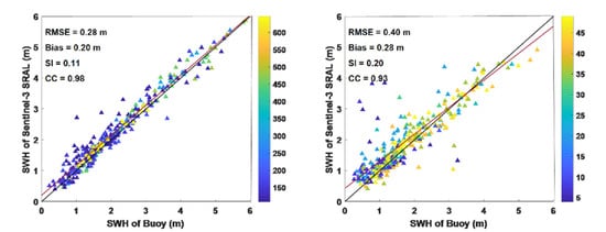
This section evaluates the accuracy of the Sentinel-3 SWH data in terms of different offshore distances. According to Table 1 and Table 2, the buoy SWH data were matched with the Sentinel-3 SWH data, and the accuracies of the two groups of data were evaluated. The results are shown in Figure 2.
As shown in Figure 2a, 15 pairs of data and 312 matching points were selected, while for Figure 2b, 16 pairs of data and 374 matching points were obtained in total, the color bar represents the distance from the coast. For the group of buoys more than 50 km offshore, the linear regression result basically coincides with the diagonal line, and the RMSE, Bias, SI, and CC are 0.28 m, 0.20 m, 0.11, and 0.98, respectively. For the group of buoys less than 50 km offshore, there is a slight deviation between the linear regression result and the diagonal line. Compared with those in Figure 2a, the RMSE, Bias and SI in Figure 2b slightly increase to 0.40 m, 0.28 m, and 0.20, respectively, while CC slightly decreases to 0.93. That is, among the indexes, the RMSE has the largest increase compared with Figure 2a, and the CC is reduced by only 0.05. These findings show that the Sentinel-3 SWH data have high accuracy in the open sea, but the accuracy is slightly reduced in coastal areas.
However, uncertainty errors always exist in these estimations, as displayed in Figure 3. The lengths of the bars in Figure 3a are mostly shorter than those in Figure 3b, which confirms that the dispersion of the SWH data more than 50 km offshore is lower than that less than 50 km offshore. By excluding data points beyond 2σ, in other words, within 2σ, for the group of buoys more than 50 km offshore, the RMSE is 0.20 m, the Bias is 0.16 m, the SI is 0.08, and the CC is 0.98; for the group of buoys less than 50 km offshore, the RMSE is 0.07 m lower, the Bias is 0.06 m lower, the SI is 0.07 lower, and the CC is 0.03 higher.
In order to estimate the relative error of Sentinel-3 SWH, Figure 4 shows the normalized error based on buoy SWH. Errors in Figure 4a are mostly below 0.2 while the errors of some buoy sites in Figure 4b are large obviously, for example C-5, C-10, and C-14, which have a short distance from the coast.
In addition, Figure 2 shows that the SWHs are concentrated mostly within the range of 0–2.5 m (light and medium waves), while some SWHs are distributed in 2.5–4 m (large waves), and the remaining SWHs are within 4–6 m (massive waves). As the SWH increases from 0 m to 6 m, Figure 2a demonstrates that the Sentinel-3 SWH data still maintain a good linear relationship with the buoy data and only slightly overestimate the observations at small SWHs; however, as shown in Figure 2b, the deviation increases to different degrees, and Sentinel-3 slightly overestimates the observations at small SWHs and underestimates the observations at large SWHs. These results confirm that Sentinel-3 can observe SWHs with high accuracy in the open sea for small to large SWHs; however, when observing nearshore waves, the data accuracy is unstable.
3.2. In Terms of Different Water Depths
This section evaluates the accuracy of the Sentinel-3 SWH data according to different buoy water depths in Table 1 and Table 2. The variations in the four evaluation indexes with the water depth are shown in Figure 5. Each panel contains 31 matching results, and Figure 5a–d present the variations in the RMSE, Bias, SI, and CC, respectively, with the water depth. To show the trends of the variations in the above indexes with the water depth intuitively and accurately, cubic curves (green lines) are used to fit the triangle symbols.
In terms of the overall distribution, the fitting curves for the RMSE, Bias, and SI show a decreasing trend with increasing water depth. The RMSE changes the most from 0.4 m to approximately 0.2 m, while the Bias changes from 0.3 m to 0.2 m, and the SI decreases from 0.2 to 0.1. The CC fitting curve has a slight increasing trend from 0.85 to approximately 0.98. The trends analyzed above reflect that the Sentinel-3 SWH accuracy increases with deeper water depths; however, the data accuracy in different regions needs to be analyzed in further detail, as discussed below.
When the water depth is more than 500 m, the RMSE value is generally less than 0.3 m, the Bias is less than 0.25 m, the SI is approximately 0.1, and the CC is approximately 0.98. When the water depth is below 500 m, Figure 5a,b indicate that the RMSE and Bias change greatly; the minimum RMSE is 0.16 m, and the maximum CC is 0.98, which reflects accurate data in deep water areas, while the maximum RMSE is 0.6 m, and the minimum CC is 0.78, which indicate low accuracy. The above analysis shows that the Sentinel-3 observation accuracy is generally high in deep waters but unstable in shallow waters; that is, the SWH can be observed with high accuracy but low accuracy in some cases. This phenomenon is similar to that described in the previous section, indicating that the offshore distance and water depth are closely related: the greater the distance from shore, the deeper the water depth, and vice versa; the shallow water case is of more concern here. Therefore, the RMSE is taken as an example, and its variation with the water depth in areas less than 50 km offshore is shown in Figure 4, which includes 18 pairs of data in total.
As shown in Figure 6, the RMSE fluctuates considerably from 0.2 m to 0.6 m in areas with water depths below 300 m; for example, the RMSEs at depths of 36.3 m and 180.7 m are both approximately 0.2 m, while the RMSEs at depths of 30 m and 200 m are greater than 0.6 m. However, the RMSEs remain stable at approximately 0.3 m in areas with water depths above 300 m. These results show that the Sentinel-3 altimeter observation accuracy is unstable in coastal areas where the water depth is shallow, while in coastal areas with relatively deep waters, the accuracy tends to remain stable. Therefore, in nearshore areas, the water depth is an important factor affecting the observation accuracy of Sentinel-3 altimetry. However, wave height in shallow water areas is also affected by wave period, so the accuracy of SWH in costal or shallow water areas observed by altimeter is more complicated to be compared with the open sea area.
3.3. In Terms of Different Coasts
This section evaluates the Sentinel-3 SWH data according to different coasts between the Pacific and Atlantic. According to Figure 1, there are 19 buoys in the Pacific and 12 buoys in the Atlantic. The matching results are shown in Figure 7, and different colors from blue to yellow represent the different distances from coasts. The normalized error based on buoy SWH of each buoy is shown in Figure 8 according to different oceans.
Figure 7a,b show that the RMSE and Bias of SWH data observed by Sentinel-3 altimeter are 0.03 m and 0.02 m, SI and CC are 0.07 and 0.03, respectively, so there is no significant difference; however, from the different colors of scattered points, it can be seen that the matching points close to the linear regression line are from blue to yellow, while the points far away from it are blue, indicating that the points with large error generally appear in the position close to the offshore. In addition, Figure 8a shows that the normalized errors of the significant wave heights of Sentinel-3 on the east coast of the Pacific Ocean are all less than 0.2, excluding the C-5 buoy station. Figure 8b shows that the normalized error ranges from 0 to 0.8 on the west coast of the Atlantic Ocean. It seems that the SWH accuracy in the Pacific is higher than in the Atlantic.
3.4. Comparison with Jason-2 Data
To verify the advantages (the high resolution) of the Sentinel-3 altimeter, the matching results with Jason-2 SWH data and buoy data at the same buoy sites are employed for a comparison with the Sentinel-3 SWH data. Table 3 shows the comparison between the Sentinel-3 and Jason-2 matching results at all the buoy locations.
From the overall results in Table 3, the Sentinel-3 RMSE is 0.35 m (0.06 m lower than the Jason-2 RMSE), the SI and Bias are both 0.02 lower than the corresponding Jason-2 indexes, and the CC is 0.02 higher. These findings suggest that the accuracy of Sentinel-3 SWH data is generally higher than that of Jason-2 SWH data, initially reflecting the former’s advantageous high accuracy.
By analyzing the matching results separately, Figure 9, Figure 10 and Figure 11 display the values of the RMSE, Bias and normalized error to visually depict the changes in the accuracy of the Sentinel-3 and Jason-2 SWH data with the water depth in areas more than 50 km and less than 50 km offshore. Figure 9a and Figure 10a correspond to the areas more than 50 km offshore, while Figure 9b and Figure 10b pertain to the areas less than 50 km offshore. On the one hand, Figure 9a and Figure 10a demonstrate that the statistical indexes (blue histogram bars) corresponding to Sentinel-3 change relatively gently with varying water depth; the RMSE ranges from 0.2 m to 0.3 m, the Bias is approximately 0.2 m. In contrast, the statistical indexes (red histogram bars) corresponding to Jason-2 change relatively violently; for example, at buoy points of L-3 m, L-11 m, and L-8 m, which are in shallow water, the RMSE and Bias of Jason-2 are obviously larger than those of Sentinel-3. However, the indexes in deep water areas change gently. At some positions, the Jason-2 indexes are better than those of Sentinel-3. On the other hand, Figure 9b and Figure 10b illustrate that the values of both the blue and the red bars fluctuate greatly, but the blue histogram bars tend to be stable when the water depth is more than 300 m. Moreover, Figure 11 shows that the normalized errors of Sentinel-3 and Jason-2 have the same tendency to each other, it has small normalized error in the area of more than 50 km offshore while it has large normalized error in some buoy sites of less than 50 km offshore. It is difficult to summarize the accuracy of the Jason-2 SWH data, whereas the Sentinel-3 SWH data accuracy is similar to that described in the last section, tending to be stable at water depths exceeding 300 m. These results show that in the open sea, the data accuracy of Sentinel-3 is higher in both shallow and deep waters, which is consistent with the conclusion in the preceding section that the accuracy is generally high. The accuracy of Jason-2 is also high in deep water but low in shallow water. In other words, the ability of Sentinel-3 to observe waves is better than that of Jason-2 at shallow water depths in the open ocean.
However, from the matching information in Table 2, there are 5 buoy sites that cannot be matched with the effective Jason-2 SWH data in areas less than 50 km offshore, at which the water depth is in the range of 0–500 m. These results are shown in Table 4, and the RMSEs are in the range of 0.29–0.48 m. This shows that the observation ability of Sentinel-3 is greatly improved in coastal areas with water depths ranging from 0 to 500 m.
The above analysis verifies that Sentinel-3 performs better than Jason-2 in shallow water areas, both in the open sea and in coastal areas. It gives expression to the advantage of high spatial resolution of Sentinel-3 altimeter, which is 300 m in the azimuthal direction; thus, Sentinel-3 can capture more wave information and fully utilize it. However, in the deep ocean with stable sea conditions, the accuracy of Jason-2 data at some positions is higher than that of Sentinel-3 data, suggesting that after many years of operation, both the parameter correction and the inversion method for traditional altimeters have developed well.
4. Conclusions
The traditional radar altimeter has the disadvantage of a low resolution, especially in nearshore observations, which are easily affected by land. The introduction of SAR technology in the Sentinel-3 altimeter enables the observation of wave information with a high resolution. The ESA evaluates the data from the Sentinel-3 altimeter worldwide, and these evaluations confirm that the data have high accuracy, but the difference in the data quality among areas with different water conditions has not been fully investigated.
In this paper, the accuracy of Sentinel-3 SWH data has been evaluated at different offshore distances and water depths and then compared with the accuracy of Jason-2 data at the same buoy sites. The accuracy evaluation results at different offshore distances show that in offshore areas, the accuracy of the data is generally high, whereas in nearshore areas, the accuracy of the data decreases to different degrees. Moreover, Sentinel-3 slightly overestimates the observations at small SWHs and underestimates the observations at large SWHs. The accuracy evaluation results at different water depths show that in deep water areas, the data accuracy is generally high, whereas in shallow water areas, the accuracy of the data is not stable and is greatly affected by the water depth, especially in shallow coastal areas, which also be related with wave period. The accuracy comparison between the two altimeters reveals that the accuracy of Sentinel-3 data is higher than that of Jason-2 data, especially in shallow water areas, but in some open sea areas with stable sea conditions, the accuracy of Jason-2 data is higher. In addition, due to the different temporal and spatial resolution between altimeter and buoy data, the average of altimeter SWH data to correspond to each buoy data also affects the evaluation of data accuracy. This work needs to be improved in the future.
Finally, considering all the results comprehensively, the Sentinel-3 altimeter can be applied to more complex sea surfaces and capture precise wave changes, but its data processing procedure is more complicated, and thus, its inversion method and data accuracy should be further improved and enhanced, especially in coastal areas.
Author Contributions
Data curation, Y.W. and R.Z.; investigation, Y.D.; resources, X.P. and C.F.; writing—original draft preparation, R.Z.; writing—review and editing, Y.W. All authors have read and agreed to the published version of the manuscript.
Funding
This work was supported in part by the National Key R&D Program of China (Grant number 2017YFC1405600).
Acknowledgments
The authors would like to thank the National Data Buoy Center for the buoy data and the EUMETSAT and AVISO+ websites for the Sentinel-3 altimeter data and Jason-2 altimeter data, respectively.
Conflicts of Interest
The authors declare no conflict of interest.
References
- Bruck, M.; Lehner, S. Coastal wave field extraction using TerraSAR-X data. J. Appl. Remote Sens. 2013, 7, 073694. [Google Scholar] [CrossRef] [Green Version]
- Zheng, C.W.; Zheng, Y.Y.; Chen, H.C. Research on wave energy resources in the Northern South China Sea during recent 10 years using SWAN wave model. J. Subtrop. Resour. Environ. 2011, 6, 54–59. [Google Scholar]
- Liang, B.C.; Fan, F.; Liu, F.S.; Gao, S.H.; Zuo, H.Y. 22-Year wave energy hindcast for the China East Adjacent Seas. Renew. Energy 2014, 71, 200–207. [Google Scholar] [CrossRef]
- Li, P.; Wu, D.H.; Li, W.X. Study of Height Estimation Algorithm on Synthetic Aperture Radar Altimeter. J. Test Meas. Technol. 2016, 30, 411–416. (In Chinese) [Google Scholar]
- Zheng, C.W.; Zhuang, H.; Li, X.; Li, X.Q. Wind energy and wave energy resources assessment in the East China Sea and South China Sea. Sci. China Technol. Sci. 2012, 55, 163–173. [Google Scholar] [CrossRef]
- Li, J.; Qian, H.B.; Li, H.; Liu, Y.; Gao, Z.Y. Numerical study of sea waves created by tropical cyclone Jelawat. Acta Oceanol. Sin. 2011, 30, 64. [Google Scholar] [CrossRef]
- Zhang, P.; Chen, X.L.; Lu, J.Z.; Tian, L.Q.; Liu, H. Research on wave simulation of Bohai Sea based on the CCMP remotely sensed sea winds. Mar. Sci. Bull. 2011, 30, 266–271. (In Chinese) [Google Scholar]
- User Guide to ECMWF Forecast Products. Available online: http://old.ecmwf.int/products/forecasts/guide/user_guide.pdf (accessed on 16 February 2013).
- Hsu, T.W.; Liau, J.M.; Lin, J.G.; Zheng, J.H.; Ou, S.H. Sequential assimilation in the wind wave model for simulations of typhoon events around Taiwan Island Hsu. Ocean Eng. 2010, 38, 456–467. [Google Scholar] [CrossRef]
- Nencioli, F.; Quartly, G.D. Evaluation of Sentinel-3A Wave Height Observations Near the Coast of Southwest England. Remote Sens. 2019, 11, 2998. [Google Scholar] [CrossRef] [Green Version]
- Gomez-Enri, J.; Vignudelli, S.; Quartly, G.D.; Gommenginger, C.P.; Cipollini, P.; Challenor, P.G.; Benveniste, J. Modeling Envisat RA-2 Waveforms in the Coastal Zone: Case Study of Calm Water Contamination. IEEE Geosci. Remote Sens. Lett. 2010, 7, 474–478. [Google Scholar] [CrossRef] [Green Version]
- Wang, X.; Ichikawa, K. Coastal waveform retracking for Jason-2 altimeter data based on along-track Echograms around the Tsushima Islands in Japan. Remote Sens. 2017, 9, 762. [Google Scholar] [CrossRef] [Green Version]
- Wingham, D.; Francis, C.; Baker, S.; Bouzinac, C.; Brockley, D.; Cullen, R.; de Chateau-Thierry, P.; Laxon, S.; Mallow, U.; Mavrocordatos, C.; et al. CryoSat: A mission to determine the flfluctuations in Earth’s land and marine ice fields. Adv. Space Res. 2006, 37, 841–871. [Google Scholar] [CrossRef]
- Fenoglio-Marc, L.; Dinardo, S.; Scharroo, R.; Roland, A.; Sikiric, M.D.; Lucas, B.; Becker, M.; Benveniste, J.; Weiss, R. The German Bight: A validation of CryoSat-2 altimeter data in SAR mode. Adv. Space Res. 2015, 55, 2641–2656. [Google Scholar] [CrossRef]
- Boy, F.; Desjonquères, J.; Picot, N.; Moreau, T.; Raynal, M. CryoSat-2 SAR-Mode Over Oceans: Processing Methods, Global Assessment, and Benefifits. IEEE Trans. Geosci. Remote. Sens. 2017, 55, 148–158. [Google Scholar] [CrossRef]
- Andriolo, U.; Mendes, D.; Taborda, R. Breaking Wave Height Estimation from Timex Images: Two Methods for Coastal Video Monitoring Systems. Remote Sens. 2020, 12, 204. [Google Scholar] [CrossRef] [Green Version]
- Almar, R.; Cienfuegos, R.A.; Catalán, P.; Michallet, H.; Castelle, B.; Bonneton, P.; Marieu, V. A new breaking wave height direct estimator from video imagery. Coast. Eng. 2012, 61, 42–48. [Google Scholar] [CrossRef]
- Yaniv, G.; Matthew, B.; Christopher, L. Automatic Estimation of Nearshore Wave Height from Video Timestacks. In Proceedings of the 2011 International Conference on Digital Image Computing: Techniques and Applications, Noosa, Australia, 6–8 December 2011; pp. 364–369. [Google Scholar]
- Sentinel-3 SRAL Marine User Handbook. Available online: https://www.eumetsat.int/wesite/wcm/idc/idcplg?IdcService=GET_FILE&dDocName=PDF_S3_SRAL_HANDBOOK&RevisionSelectionMethod=LatestReleased&Rendition=Web (accessed on 5 May 2019).
- Birgiel, E.; Ellmann, A.; Delpeche-Ellmann, N. Examining the Performance of the Sentinel-3 Coastal Altimetry in the Baltic Sea Using a Regional High-Resolution Geoid Model. In Proceedings of the 2018 Baltic Geodetic Congress (BGC Geomatics), Olsztyn, Poland, 21–23 June 2018; pp. 196–201. [Google Scholar] [CrossRef]
- Delikaraoglou, D.; Flokos, N. Preliminary assessment of observing different regime-s in the marine environment using SENTINEL-3 data. Earth Space Sci. Open Arch. 2019. [Google Scholar] [CrossRef]
- Gao, Q.; Makhoul, E.; Escorihuela, M.J.; Zribi, M.; Quintana Seguí, P.; García, P.; Roca, M. Analysis of Retrackers’ Performances and Water Level Retrieval over the Ebro River Basin Using Sentinel-3. Remote Sens. 2019, 11, 718. [Google Scholar] [CrossRef] [Green Version]
- Jiang, L.G.; Nielsen, K.; Dinardo, S.; Andersen, O.B.; Bauer-Gottwein, P. Evaluation of Sentinel-3 SRAL SAR altimetry over Chinese rivers. Remote Sens. Environ. 2020, 237, 111546. [Google Scholar] [CrossRef]
- Yang, J.G.; Zhang, J. Validation of Sentinel-3A/3B Satellite Altimetry Wave Heights with Buoy and Jason-3 Data. Sensors 2019, 19, 2914. [Google Scholar] [CrossRef] [Green Version]
- Sentinel-3-MPC-ECM-Winds-Waves-Cyclic-Report-050-031. Available online: https://sentinel.esa.int/documents/247904/3748263/Sentinel-3-MPC-ISR-SRAL-Cyclic-Report-050-031.pdf (accessed on 26 December 2019).
- Ray, C.; Martin-Puig, C.; Clarizia, M.P.; Ruffini, G.; Dinardo, S.; Gommenginger, C.; Benveniste, J. SAR Altimeter Backscattered Waveform Model. IEEE Trans. Geosci. Remote Sens. 2015, 53, 911–919. [Google Scholar] [CrossRef]
- OSTM_Jason-2 Products Handbook. Available online: https://www.ospo.noaa.gov/Products/documents/J2_handbook_v1-8_no_rev.pdf (accessed on 10 January 2020).
- Han, X.; Yang, J.G.; Wang, J.Z. Calibration and evaluation of satellite radar altimeter wave heights with in situ buoy data. Acta Oceanol. Sin. 2016, 38, 73–89. (In Chinese) [Google Scholar]
Figure 1.
Study areas and buoy site locations (blue triangles indicate buoys more than 50 km offshore, yellow circles indicate buoys less than 50 km offshore).
Figure 1.
Study areas and buoy site locations (blue triangles indicate buoys more than 50 km offshore, yellow circles indicate buoys less than 50 km offshore).

Figure 2.
Matching results of the Sentinel-3 and buoy data: (a) more than 50 km offshore and (b) less than 50 km offshore (with the 45° diagonal line in black and the linear regression result in red).
Figure 2.
Matching results of the Sentinel-3 and buoy data: (a) more than 50 km offshore and (b) less than 50 km offshore (with the 45° diagonal line in black and the linear regression result in red).

Figure 3.
Box plot figure of uncertainty errors of each group of data: (a) more than 50 km offshore and (b) less than 50 km offshore (with yellow squares in the middle of each bar represent the mean of the Bias between a group of Sentinel-3 and buoy significant wave height (SWH) data, and the upper and lower limits of the bars represent the mean value plus or minus the standard deviation (σ), respectively).

Figure 4.
Normalized error based on Buoy SWH: (a) more than 50 km offshore and (b) less than 50 km offshore.
Figure 4.
Normalized error based on Buoy SWH: (a) more than 50 km offshore and (b) less than 50 km offshore.

Figure 5.
Evaluation index variations with water depth: (a) RMSE, (b) Bias, (c) scattering index (SI), and (d) correlation coefficient (CC) (with the fitted cubic curve in green).
Figure 5.
Evaluation index variations with water depth: (a) RMSE, (b) Bias, (c) scattering index (SI), and (d) correlation coefficient (CC) (with the fitted cubic curve in green).

Figure 6.
Variation in the RMSE with the water depth in areas less than 50 km offshore.

Figure 7.
Matching results of the Sentinel-3 and buoy data: (a) Pacific and (b) Atlantic.

Figure 8.
Matching results of the Sentinel-3 and buoy data: (a) Pacific and (b) Atlantic (red points represent buoys less than 50 km offshore and blue points represent buoys more than 50 km offshore).
Figure 8.
Matching results of the Sentinel-3 and buoy data: (a) Pacific and (b) Atlantic (red points represent buoys less than 50 km offshore and blue points represent buoys more than 50 km offshore).

Figure 9.
Variations in the RMSEs of Sentinel-3 and Jason-2 SWH data with the water depth: (a) more than 50 km offshore and (b) less than 50 km offshore.
Figure 9.
Variations in the RMSEs of Sentinel-3 and Jason-2 SWH data with the water depth: (a) more than 50 km offshore and (b) less than 50 km offshore.

Figure 10.
Variations in the Biases of Sentinel-3 and Jason-2 SWH data with the water depth: (a) more than 50 km offshore and (b) less than 50 km offshore.
Figure 10.
Variations in the Biases of Sentinel-3 and Jason-2 SWH data with the water depth: (a) more than 50 km offshore and (b) less than 50 km offshore.

Figure 11.
Normalized error of Sentinel-3 and Jason-2: (a) more than 50 km offshore and (b) less than 50 km offshore.
Figure 11.
Normalized error of Sentinel-3 and Jason-2: (a) more than 50 km offshore and (b) less than 50 km offshore.


Table 1.
Information of buoys more than 50 km offshore.
| Buoy Number | Buoy ID | Depth (km) | Distance from the Coast (km) | S3 Track | J2 Track |
|---|---|---|---|---|---|
| L-1 | 46066 | 4 | 334 | 305 | 199 |
| L-2 | 51004 | 5 | 196 | 063 | 158 |
| L-3 | 46005 | 3 | 485 | 076 | 130 |
| L-4 | 46073 | 3 | 195 | 163 | 175 |
| L-5 | 46035 | 4 | 462 | 206 | 056 |
| L-6 | 46089 | 3 | 164 | 361 | 028 |
| L-7 | 46001 | 4 | 275 | 114 | 054 |
| L-8 | 46080 | 0.25 | 109 | 328 | 054 |
| L-9 | 46085 | 4 | 437 | 071 | 173 |
| L-10 | 46078 | 5 | 121 | 148 | 156 |
| L-11 | 44008 | 0.08 | 116 | 259 | 065 |
| L-12 | 41010 | 1 | 183 | 011 | 243 |
| L-13 | 41013 | 0.03 | 111 | 011 | 076 |
| L-14 | 42039 | 0.27 | 152 | 268 | |
| L-15 | 41040 | 5 | 647 | 002 | 063 |
Table 2.
Information of buoys less than 50 km offshore.
| Buoy Number | Buoy ID | Depth (km) | Distance from the Coast (km) | S3 Track | J2 Track |
|---|---|---|---|---|---|
| C-1 | 46029 | 0.13 | 26 | 090 | |
| C-2 | 46011 | 0.46 | 43 | 033 | |
| C-3 | 46083 | 0.14 | 35 | 019 | 173 |
| C-4 | 46082 | 0.30 | 42 | 119 | 104 |
| C-5 | 51201 | 0.20 | 21 | 277 | 223 |
| C-6 | 46069 | 1 | 49 | 027 | 206 |
| C-7 | 46086 | 2 | 41 | 198 | |
| C-8 | 46072 | 4 | 48 | 343 | 234 |
| C-9 | 44007 | 0.03 | 20 | 259 | 202 |
| C-10 | 44009 | 0.03 | 4 | 011 | 228 |
| C-11 | 44025 | 0.04 | 12 | 011 | 243 |
| C-12 | 41025 | 0.06 | 31 | 011 | 076 |
| C-13 | 44005 | 0.18 | 48 | 068 | 050 |
| C-14 | 41008 | 0.01 | 7 | 168 | |
| C-15 | 46012 | 0.21 | 46 | 361 | |
| C-16 | 46084 | 1 | 36 | 085 | 071 |
Table 3.
Accuracy verification results of Sentinel-3 and Jason-2 SWH data.
| Satellite | RMSE (m) | CC | SI | Bias (m) | Number of Matching Buoys | Number of Matching Points |
|---|---|---|---|---|---|---|
| Sentinel-3 | 0.35 | 0.96 | 0.16 | 0.24 | 31 | 686 |
| Jason-2 | 0.41 | 0.94 | 0.18 | 0.26 | 25 | 912 |
Table 4.
Accuracy verification results between the Sentinel-3 and buoy sites for which Jason-2 cannot obtain effective SWH data.
Table 4.
Accuracy verification results between the Sentinel-3 and buoy sites for which Jason-2 cannot obtain effective SWH data.
| Buoy ID | RMSE (m) | Bias (m) | SI | CC |
|---|---|---|---|---|
| 46029 | 0.45 | 0.27 | 0.19 | 0.94 |
| 46011 | 0.36 | 0.27 | 0.15 | 0.91 |
| 46086 | 0.29 | 0.21 | 0.21 | 0.87 |
| 41008 | 0.33 | 0.3 | 0.24 | 0.82 |
| 46012 | 0.48 | 0.4 | 0.15 | 0.94 |
© 2020 by the authors. Licensee MDPI, Basel, Switzerland. This article is an open access article distributed under the terms and conditions of the Creative Commons Attribution (CC BY) license (http://creativecommons.org/licenses/by/4.0/).
Share and Cite
MDPI and ACS Style
Wan, Y.; Zhang, R.; Pan, X.; Fan, C.; Dai, Y. Evaluation of the Significant Wave Height Data Quality for the Sentinel-3 Synthetic Aperture Radar Altimeter. Remote Sens. 2020, 12, 3107. https://doi.org/10.3390/rs12183107
AMA Style
Wan Y, Zhang R, Pan X, Fan C, Dai Y. Evaluation of the Significant Wave Height Data Quality for the Sentinel-3 Synthetic Aperture Radar Altimeter. Remote Sensing. 2020; 12(18):3107. https://doi.org/10.3390/rs12183107
Chicago/Turabian StyleWan, Yong, Rongjuan Zhang, Xiaodong Pan, Chenqing Fan, and Yongshou Dai. 2020. "Evaluation of the Significant Wave Height Data Quality for the Sentinel-3 Synthetic Aperture Radar Altimeter" Remote Sensing 12, no. 18: 3107. https://doi.org/10.3390/rs12183107
Note that from the first issue of 2016, this journal uses article numbers instead of page numbers. See further details here.