Article

Riverine Sediment Changes and Channel Pattern of a Gravel-Bed Mountain Torrent

by
Gernot Seier
1,*,
Stefan Schöttl
2,
Andreas Kellerer-Pirklbauer
1,
Raphael Glück
1,
Gerhard K. Lieb
1,
Daniel N. Hofstadler
3 and
Wolfgang Sulzer
1
1
Department of Geography and Regional Science, University of Graz, 8010 Graz, Austria
2
Federal Research and Training Centre for Forests, Natural Hazards and Landscape (BFW), 1131 Vienna, Austria
3
Institute of Biology, University of Graz, 8010 Graz, Austria
*
Author to whom correspondence should be addressed.
Remote Sens. 2020, 12(18), 3065; https://doi.org/10.3390/rs12183065
Submission received: 27 July 2020 / Revised: 14 September 2020 / Accepted: 16 September 2020 / Published: 19 September 2020
(This article belongs to the Special Issue Remote Sensing for Geomorphological Mapping)

Abstract

:
The alluvial channel of the Langgriesgraben (Austria) is a highly active geomorphic riverine subcatchment of the Johnsbach River with intermittent discharge and braided river structures. The high sediment yield entails both issues and opportunities. For decades, the riverbed was exploited as a gravel pit. Today, as part of the Gesäuse National Park and after renaturation, the sediment yield endangers a locally important bridge located at the outlet of the subcatchment. High-resolution geospatial investigations are vital for the quantification of sediment redistribution, which is relevant in terms of river management. Based on unmanned aerial system (UAS) surveys in 2015 (July, September, and October) and 2019 (August and October), high-resolution digital elevation models (DEMs) were generated, which enable us to quantify intra- and multiannual sediment changes. As surface runoff at the subcatchment occurs on only a few days per year with flash floods and debris flows that are not predictable and thus hardly observable, the subsurface water conditions were assessed based on electrical resistivity tomography (ERT) measurements, which were conducted in 2019 (November) and 2020 (May, June). Results of the UAS-based surveys showed that, considering the data quality, intra-annual sediment changes affected only small subareas, whereas multiannual changes occurred in the entire study area and amount to net sediment deposition of ≈0.3–0.4 m3m−2, depending on the channel section. In addition, the elevation differences for both intra-annual surveys revealed linear patterns that can be interpreted as braided river channels. As in both survey periods the same areas were affected by changes, it can be concluded that the channel mainly affected by reshaping persisted within the 4-year observation period. The subsurface investigations showed that although both near-surface and groundwater conditions changed, near-surface sediments are mostly dry with a thickness of several meters during the observations.

Graphical Abstract

1. Introduction

Fluvial landforms are of great importance from an ecological and economical perspective. Fluvial processes vary greatly in size, dimension, and intensity: floods regularly threaten engineered constructions and even human lives, while plenty of small-scale, short-term changes often go unrecognized. Riverine landforms form where water runs as overland flow and streamflow in river channels, which is based on runoff production as the difference between precipitation and evaporation rates [1] and relates to the removal and transfer of Earth surface materials [2]. In this study, we focus on the lower section of the gravel-bed braided mountain torrent Langgriesgraben, which is affected by high geomorphic activity related to periods of intermittent discharge.
Today, humans are considered geomorphological agents in riverine systems and channel reshaping could entail increased fluxes of water and sediments [3]. However, extricating human impact from natural processes is challenging [4]. Remote sensing techniques are not only scientific tools but are relevant for river management at local to basin scales [5]. In the Langgriesgraben area, which is a branch of the Johnsbach River, gravel mining coined the channel morphology for decades [6]. In 2010, renaturation measures were carried out and since then, natural processes of erosion and deposition cause the reshaping of the channel. At the Langgriesgraben, the channel and downstream movement of sediments threaten a bridge and traffic pathway crossing the mountain torrent at the channel outlet [7].
Research on gravel-mining-induced river changes provides the basis for adjusting adequate management concepts [8,9]. While discharge measurements give basic insights into channel geometry [10], the most reliable recordings considering the geospatial context are measured in situ. Due to vegetation cover and the rapid change of streambank topography, the geomorphic monitoring and analysis of riverine processes is often challenging [11]. However, the use of high-resolution geospatial methods to investigate fluvial morphology is increasing. Contemporary methods of reconstructing streambank topography are the use of unmanned aerial systems (UASs) and airborne and terrestrial laser scanning (ALS, TLS) [11,12]. The methodological approach of choice often depends on technical constraints, local terrain conditions, and the costs. ALS facilitates the surveying of large areas, but only with a comparably low ground resolution (the typical ground sampling distance of the digital elevation model, DEM, is 0.5–1 m). On the other hand, TLS generate very high-resolution, accurate datasets. However, the surveying of complex terrain with TLS requires appropriate scan positions in order to avoid data gaps (scan shadow) and misinterpretation of geomorphic changes. UAS are in many cases better suited for small-scale geomorphic investigations particularly in unvegetated areas, although there are several disadvantages compared to TLS and airborne (manned airplanes) approaches, such as challenging flight environments, limits of on-board power, limited payload and challenges in processing and analyzing the imagery [13]. UAS are beneficial in inaccessible areas to gain insights for visual interpretation [14]. For image-based surface reconstruction, UAS in conjunction with Structure-from-Motion (SfM) photogrammetry entails added value [15] at low costs compared to ALS or TLS. Recent years were characterized by an increasing number of articles dealing with SfM photogrammetry [16]. For geomorphic change detection in riverine landscapes, UAS and SfM photogrammetry have been introduced and have proven an important tool for quantifying complex fluvial terrain, e.g., [4,17,18,19]. A combination of ground-based and airborne measurements in Earth observation is worth striving for and TLS are often used in terms of validation and reference, e.g., [17,20,21]. As each technique is prone to different drawbacks, integrated approaches avoid misinterpretations in studying 3D geometry [22]. In addition, the combined use of UAS-based measurements with geophysical methods is beneficial as limitations of each method can be assessed [23]. In particular, a combination of electrical resistivity tomography (ERT) measurements with other geophysical [24] and UAS-based results can help to more suitably interpret subsurface and surface conditions [25]. SfM approaches require the appropriate photogrammetric processing, which comprises the adequate reporting of the data quality, survey design, flight campaigns and processing [26,27,28]. This enables reliable reconstruction of topography [29,30]. In fluvial morphology, investigations of morphodynamic processes such as erosion and deposition and related changes are currently often conducted by the use of UAS, e.g., [31,32,33].
With this study we intend to (i) detect intra- and multiannual sediment changes of a gravel-bed channel, (ii) reveal consequences of methodological issues of UAS-based SfM photogrammetry in studying riverine changes by confronting the results gathered through UAS-based SfM photogrammetry with their inherent uncertainties, (iii) address the question of how the braided channel pattern formed over the course of 4 years, and (iv) shed light on the channel’s subsurface conditions as surface runoff at the study site is hardly observable.

2. Study Area

The Langgriesgraben (literally translated ‘long debris trench’) area is a 3.3 km2 large subcatchment of the Johnsbach River and is located in the Gesäuse National Park, Austria (14°34′31′’E, 47°33′37′’N, Figure 1a and Figure 2). The subcatchment of the Langgriesgraben area (Figure 1b), which belongs to the Northern Limestone Alps, is geologically characterized by alluvium (Holocene), breccia (Holocene) and a sequence of Wetterstein dolomite, limestone schists, and Dachstein dolomite (all Triassic). The gravel-bed channel is in its lower reaches dominated by unconsolidated rock (Holocene).
Within the Langgriesgraben area, this study focuses on a section of 1.1 km in length reaching from the bridge close to the Johnsbach River to the junction with the Schwarzschiefergraben entering from the south (Figure 1a and Figure 2a). The riverbed of the Langgriesgraben is a highly active geomorphological area [34,35,36,37], that has been influenced by gravel mining over the course of several decades, which began at least in the 1970s but probably even after World War II [6]. In 2009 and 2010 renaturation measures were carried out [37]. Since then, the Langgriesgraben has been undergoing natural processes of erosion and deposition of unconsolidated sediments [37,38]. The alluvial channel of the Langgriesgraben is characterized by braided structures (Figure 2). Surface runoff is prevalent on only a few days per year caused by rainstorms, which result in flash floods (see Figure 2d,e personal correspondence with local residents and the Gesäuse National Park management). Indications for perennial surface runoff, which are based on field evidence of observations in October 2019 as well as May and June 2020, are evident a bit uphill of the area investigated (Figure 1a). During the period of the study’s measurements (31 July 2015–06 June 2020) the precipitation at the nearest rain gauge (Weidendom) was characterized by seasonal variations with clear maxima (of up to ≈65 mm d−1) in the summer months (Figure 3). Water discharge measurements at the nearest water gauge (Gsengbrücke) reflect the seasonality of discharge with maxima of up to ≈11 m3 s−1, even though the measurements appear distorted as of September 2018 because in the former years water discharge was detectable throughout the entire period (Figure 3), and which is a known issue caused by bedload (personal correspondence with the gauge maintaining personnel).

3. Materials and Methods

3.1. Survey Design and Data Acquisition

3.1.1. Unmanned Aerial System-Based Survey

The area covered with the use of UAS measures ≈17 ha and the channel investigated is ≈3.5 ha large (Figure 1a, white outline). Five flight campaigns in 2015 and 2019 were conducted using two different multirotor UAS (Table 1). Due to still unknown technical issues with the UAS in the first two field campaigns (July and September 2015), the area covered was remarkably smaller than the planned area. This uncovered area was then covered with a separate flight campaign in October 2015 (Figure 1a) and this is why these subareas are presented in separate maps. The planned image overlap was 80% forward and 60% side. By taking into account the actual average height above ground (nadir of perspective center) of ≈79–≈111 m, at nadir points ground sampling distances (GSD) of ≈0.02 and ≈0.04 m resulted (Table 1), irrespective of the rather slight slope gradient. During the acquisition of the vertically oriented photographs, the UAS stopped at so-called waypoints. The cameras used are a Ricoh GXR A12 and the integrated DJI Phantom 4 camera. The resolution of the consumer grade Ricoh camera with a focal length of 18.3 mm (fixed manual focus set at infinity) is 4288 × 2848 pixels (px). The size of the camera’s sensor (Ricoh) is 23.6 × 15.7 mm (≈371 mm2), which gives a pixel size of ≈5.5 µm. The DJI camera’s sensor is characterized by a size of 6.3 × 4.7 mm (≈30 mm2), a resolution of 4000 × 3000 px (pixel size of ≈1.58 µm), and a focal length of 3.61 mm. Using the Ricoh camera, the shutter speed was fixed (shutter priority) to 1/1000 s during all three surveys in 2015, as recommended, e.g., [39]. The DJI camera used in the 2019 surveys was not widely adjustable and was used in auto focus mode.
As the areas covered using the UAS varied and the cameras used differed, the number of photographs taken ranged from 31 images for a single flight to 190 images for the entire area covered by three flights (Table 1). The camera mounting of the hexacopter UAS does not allow for off-nadir image capture and it was not possible to acquire convergent imagery. The DJI camera would have made it possible to taking oblique imagery but due to efforts required for field work there was not enough time to conduct additional flights.
Signalized objects that are only viewed from a restricted range of angles cause precisions that are significantly reduced along the viewing axis, e.g., [40,41]. The achievable precision in the viewing direction, σ z , can be estimated by
σ z =   D ¯ 2 b d σ i
where D ¯ is the mean object distance, σ i is the precision of image measurements (assumed to be a half pixel), b is the distance between the camera centers (i.e., the stereo base), and d is the principal distance of the camera. According to [41], the achievable object precision parallel to the image plane, σ x (= σ y ), can be estimated by
σ x =   m b   σ i
where m b is the image scale number (calculated by D ¯ d ). Considering the intersecting geometry of the imaging configuration, this object precision can be weighted by introducing a design factor q [42], which can be up to a value of 3.0 for weak imaging configurations [41]. Table 1 shows the according estimated precision values.

3.1.2. Electrical Resistivity Tomography

Electrical resistivity is a physical parameter related to the chemical composition of a material and its porosity, temperature, water, and ice content [43]. The principle of electrical resistivity tomography (ERT) is based on electric current that is directly injected into the ground using a pair of electrodes [44]. Consequently, voltage between another pair of electrodes is measured. The impedance of the Earth is derived (which is the ratio of the voltage output measured to the current input) and transformed to apparent resistivity (Ωm). This apparent resistivity is an indicator of the actual underlying electrical resistivity structure of the Earth [44].
For ERT, we used a multi-electrode system (GeoTom, Geolog, Germany) and two-dimensional data inversion (Res2Dinv) for data analysis. For this study, a 196 m long cross profile at the lower section of the study area was chosen for repeated measurements (Figure 1a, Table 2). This profile covers the entire gravel-bed braided river system and the adjacent terrace structures. At the southern end, the profile ends close to bedrock. Along the entire profile 50 electrodes (metal rods) with 4 m spacing in between were installed during the measurements. For the central part of the profile, a more detailed measurement setup was applied with only 2 m spacing between two adjacent electrodes (Table 2). We applied mainly the Wenner array (partly also Schlumberger for cross-check) because this array is more suitable for layered structures as can be expected in water-related research questions [43].

3.1.3. Geodetic Measurements

For processing the UAS-based photographs and for accuracy assessment, geodetic surveys using a Global Navigation Satellite System (GNSS) receiver (Topcon HiPerV dual-frequency) and Real Time Kinematics (RTK) corrections via EPOSA [45] accompanied the UAS surveys. Thus, ground control points (GCPs) as signalized points were measured for each flight campaign, which is required for indirect georeferencing of the UAS images. The spatial distribution of GCPs for each flight campaign is shown in Figure 4. The precision of the position measurement is 0.02–0.03 m horizontally and 0.03–0.05 m vertically (personal correspondence, Wiener Netze GmbH 2017). In addition to these GCPs so-called independent check points (ICPs) were surveyed in the field campaigns using the same technique. The ICPs differ from GCPs, as these are not signalized points and serve to independently verify the vertical accuracy of the finally generated DEMs (see Section 4.1.2). GNSS was also used to measure each electrode location during the ERT campaigns and thus the course of the ERT profile.

3.1.4. Terrestrial Laser Scanning Data

For accuracy assessment of the UAS-based results of October 2015, which was not accompanied by GNSS measurements, terrestrial laser scanner (TLS) measurements were conducted on 13 October 2015 to independently assess the quality of the UAS-based results. By sending out a laser beam that is reflected by the surface covered, a TLS measures the distance from the device to the surveyed surface and thus 3D coordinates for each surveyed point are derived from the range measurement, the horizontal direction and the vertical angle. Consequently, point clouds are generated that are internally referenced and need to be georeferenced [46,47].
The device used is a Riegl laser scanner LMS-Z620, which was designed for survey ranges of up to 2000 m [48]. The data processing was performed in RiScanPro (Version 2.1.1) and can be summarized as follows: target-based registration of the scan positions (project coordinate system), filtering and manual cleaning of the point cloud data, georeferencing of the point cloud via GNSS measured targets and export of the point cloud for further analysis. Further details are presented in [38] and [49].

3.2. Photogrammetric Processing

The processing of the UAS-based photographs is based on SfM [50] photogrammetry. The SfM photogrammetry approach uses photographs captured from different perspectives and these photographs are then automatically assembled to point clouds using image matching techniques. This matching uses the identification of interest points and is based on the Scale-Invariant Feature Transform [51] algorithm. In combination with multi-view stereo (MVS) techniques, SfM photogrammetry enables simultaneous reconstruction of dense 3D models, camera positions, and orientations [52]. Recently, SfM-MVS photogrammetry became increasingly used in a variety of geoscientific fields, e.g., [53,54,55,56,57].
The SfM photogrammetry approach was implemented using the commercial software Agisoft Metashape (v. 1.5.3). Data processing was conducted by generating a sparse point cloud in a first step (feature matching in photos to estimate camera positions and orientations), followed by a bundle adjustment, and finally, a dense point cloud was generated with so-called aggressive depth filtering, which means that small surface details are not considered because they possibly show model-induced errors. The following processing settings were chosen: a default key point limit of 40,000 and a default tie point limit of 4000. The camera parameters such as focal length, principal point offsets (cx, cy), and radial distortion (K1, K2, K3) were set to adjustable in the process of camera self-calibration. The projection accuracy (i.e., the precision of GCPs on the image plane) was set to 0.5 pixel. The measurement precision of the GCP coordinates on the observed surface (in the software referred to as ‘marker accuracy’) was set to 0.0075 m (as a general value and as the software description recommends a divisor of 4 to be applied to the measurement precision). The dense point clouds were exported to raster files (orthophotos and DEMs) with GSDs of 0.02–0.04 m.

4. Results

4.1. Accuracy Assessment

4.1.1. Ground Control Points

For assessing the quality of the photogrammetric processing, the horizontal (XY) and vertical (Z) root mean square errors (RMSEs) of the GCPs were used. The GCPs’ XY RMSEs are in the range of 0.02–0.04 m and the Z RMSEs are in the range of 0.03–0.05 m, which gives total RMSEs (XYZ) of 0.03–0.07 m. The residuals are graphically presented in Figure 4. Almost all horizontal residuals stay within the range of a few centimeters, and the vertical residuals are in the same order of magnitude. For all UAS-based results, the spatial distributions of the residuals follow no discernible pattern (Figure 4). Therefore, the residuals indicate that the georeferencing was conducted adequately.

4.1.2. Independent Check Points

Independent GNSS measurements are of prime importance to assess the quality of DEMs from SfM photogrammetry. In the 2019 field campaigns, such independent check points (ICPs) were recorded for all flight campaigns on the same day as the UAS flights (Figure 5). However, the UAS-based data of 2015 were partially compared to TLS measurements (October 2015, see Section 4.1.3), whereas the July and September 2015 flight campaigns were accompanied by only few such ICP measurements (covering small subareas) in a follow-up survey on 3 November 2015 (because of the limited satellite availability in the deeply incised channel and the fact that in the July and September 2015 flight campaigns, technical issues with the UAS entailed time-consuming support queries).
Elevation differences of ICPs (n = 33) measured on 3 November 2015 were compared with elevations of the UAS-based DEM (ICP elevations subtracted from DEM) of July 2015, which resulted in a mean difference of −0.06 m and standard deviation (SD) of 0.06 m. Compared to the UAS-based elevations of September 2015, these ICPs gave a mean of 0.10 m and SD of 0.075 m. For the August 2019 survey, the elevation differences of the ICP measurements and the particular DEM are characterized by a mean of −0.01 m and SD of 0.03 m (n = 142). For the October 2019 survey, a mean of −0.07 m and SD of 0.04 m (n = 65) were found. These SD values were then used to determine the threshold for the differentiation of meaningful results from possibly model-induced errors. Using the highest SD value from all the DEMs generated (0.075 m) as the error metric, the uncertainty range of a single DEM was estimated with ±0.15 m (2 × SD). This was used as a basis for the rather conservative estimate of the threshold of meaningful elevation differences, which was set to ±0.30 m (Section 4.2) as double the 2 × SD value for a single DEM. The principle of error propagation would allow for a lower threshold, but we opted for a stricter (higher) one to focus on the most substantial results (Section 5.1.2).

4.1.3. Comparison of TLS with UAS Data

For the UAS flight campaign in October 2015 an independent quality assessment was conducted based on three subareas (A–C) covered by TLS data (measured on 13 October 2015, Figure 5). The subarea A is located on an adjacent slope of the channel and subareas B and C are located in the riverbed. The temporal offset between the UAS and TLS data acquisition of 9 days should be neglectable as no extraordinary precipitation at the rain gauge Weidendom (for location see Figure 1c) occurred (Figure 3).
The comparison was conducted using DEM differencing. The UAS-based DEM was subtracted from the TLS-based DEM. In the subareas B and C, a systematic offset of the UAS data can be observed (Figure 5). This visual interpretation is confirmed by a clear positive mean difference for these two small sites (Table 3), which indicates that the UAS-based elevations are generally slightly lower than the TLS-based elevations. Details of the data preparation are presented in [36].

4.2. Elevation Differences

The intra-annual elevation differences from 2015 and 2019 are shown in Figure 6a,b. In 2015 (during a 53 days lasting period from July to September), the far eastern and lower section of the Langgriesgraben generally shows only minor changes, with some exceptions of notable net erosion and deposition (Figure 6a). Similarly, only small subareas were affected by noteworthy changes (Figure 6b) in the UAS-based results of 2019 (9 August–17 October, 69 days).
The multiannual elevation differences from 2015 and 2019 are shown in Figure 6c,d. The far east part and lower section of the Langgriesgraben underwent net accumulation to a thickness of up to ≈0.5–2 m during the years 2015–2019 (July 2015 and August 2019, Figure 6c). The western and uppermost section of the study area shows similar but slightly more distinct changes due to erosion and deposition in the period from October 2015 to October 2019 (Figure 6d).

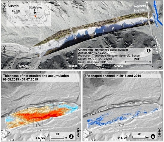
4.3. Evidence of Bank Erosion

The deposited sediments originate from further up the valley and from adjacent slopes, as evident comparing orthophotos from 2015 and 2019 (Figure 7). Erosion and displacement of the riverbank amounted to up to ≈1–3 m on both sides of the channel. For instance, alongside a steep slope located in the uppermost north-western section of the study area loose sediment was deposited (Figure 7c). In addition, changing braided river structures are recognizable (Figure 7).

4.4. Volumetric Changes

Based on the elevation differences, the volumetric changes were calculated for the corresponding periods of time and different subareas (Table 4). In both the intra-annual and multiannual cases deposition exceeded erosion. A further discussion on the effect of different thresholds used (to distinguish noise from actual change) is presented in Section 5.1.3.

4.5. Subsurface Conditions

The ERT measurements give insight into the changes of subsurface water conditions between November 2019 and June 2020 (Figure 8). According to [58], resistivity values in the range of 100 (humid and fractured limestone) to >100,000 Ωm (very compact limestone) can be expected for limestone rocks. [59] measured resistivity values of 10,000–30,000 Ωm for unfrozen and compact Wetterstein limestone. Furthermore, the authors of [60] measured 3000–28,000 Ωm for compact and unweathered Dachstein limestone. The two long profiles measured in November 2019 and June 2020 revealed bedrock at the southern end and along the first third of the profile with values exceeding 10,000 Ωm, which is a reasonable estimate value for fractured limestone and dolomite as outlined above. The sediment thickness at the southern section of the long profiles is in the order of 20 m, whereas at the northern section sediments exceed depths of 30 m. The superficial layer of higher resistivity values is related to dry sediments with air voids in between. In November 2019, this layer was about 2 m thick at the streambed covering a groundwater-filled sediment body. On 15 May 2020, the upper 10 m of the sediments in the riverbed dried out causing a lowering of the groundwater table as indicated by values exceeding 4000 Ωm. However, close to the surface (i.e., upper 5 m) the sediments revealed higher resistivity values compared to November 2019 indicating moistening. About 3 weeks later (6 June 2020), subsurface conditions changed again with lower resistivity values also closer to the surface of the streambed indicating an increase of the water table. However, the comparison of the November 2019 data (both short and long profiles) with the June 2020 data shows that the subsurface channel was more water-saturated in late autumn compared to late spring and early summer.

5. Discussion

5.1. Quality of Data and Analysis

5.1.1. Estimation of Survey Quality

With this section we aim to discuss the quality of the data and potential implications. Issues faced in topographic studies of complex terrain are seldom reported [61]. Several survey steps involve factors that, if not carefully managed, could reduce the study’s meaningfulness, such as the flight planning, e.g., [62].
The estimated achievable precisions of the five UAS surveys range from σ x = ≈0.04 to ≈0.06 m and σ z = ≈0.07 to ≈0.12 m. Compared to the GCPs’ (total) RMSEs of all surveys, which range from 0.03 to 0.07 m, these estimated precision values correspond with the actually achieved values (Table 5). We therefore can assume that the surveys were adequately planned and conducted. In addition, the ICPs’ height precision values (SD = 0.03–0.075 m) confirmed the estimated achievable precisions. Furthermore, relative precision ratios (ratio of the theoretical estimate σ z to D ¯ ) of ≈1:1000 are achievable in SfM-MVS studies, not only in traditional stereo photogrammetry [63,64]. In our case, estimated precision ratios (of σ z to camera distance) are actually in the range of ≈1:1000 or slightly below, which is a result of the flight height above ground and the camera used (Table 5).
Moreover, in a range of SfM-related studies, ratios of RMSE to a survey range of 1:639 are reported [65]. In our case, these ratios are in a range of ≈1:1045–≈1:1305 (Table 5), which is a further indication of the expected and adequate accuracy of our results.

5.1.2. Implications of the Survey Quality for the Interpretation

Due to error propagation the chosen threshold of elevation differences used (±0.30 m) to distinguish actual change from noise could overestimate errors (Section 4.1.2). On the other hand, this approach could be interpreted as conservative estimate, which means that difference values exceeding even this threshold are more reliably showing change. However, in terms of estimating the data quality for the elevation difference calculations, the following equation can be used to consider the propagation of error (see [66]):
E Diff = t   S D D E M 1 2 +   S D D E M 2 2
where EDiff is the error estimate used as threshold, SDDEM1 and SDDEM2 are the standard deviations of errors in each DEM, and t is the critical t-value (of 1.96) at the chosen confidence level of 95%. Considering the same SD value as in Section 4.1.2 of 0.075 m and additionally SD of 0.05 m (which could be applicable as this value is in between the different SD values resulting from ICPs) would then give thresholds of ±0.21 and ±0.14 m.
Considering different thresholds to distinguish noteworthy elevation changes from noise results to some extent in totally different areal coverage, whereas other subareas of the study area are not influenced by the data’s uncertainties (Figure 9). Here, the intra-annual elevation differences of the lower and far eastern section of the Langgriesgraben would be clearly affected by elevation differences in the 2015 survey if the threshold was remarkably lower. Hence, this would lead to the conclusion that most of the study area changed in the particular period of time (Figure 9a). The other cases, namely the 2019 survey (Figure 9b) and the larger threshold used (Figure 9c,d), would not lead to different visually based interpretations. The multiannual elevation differences are not further discussed as the elevation differences are generally far above the thresholds in question.

5.1.3. Volume Calculations

The consequences of uncertainties on volume calculations are depicted in Figure 10, which is based on the conservative threshold of ±0.30 m (see Section above and Section 4.1.2).
As the intra-annual elevation differences were to a large extent not meaningful compared to the threshold used to distinguish change from possible error (see Figure 6) or slightly above the threshold, the uncertainties directly influence the calculated volume (Figure 10). Hence, in both intra-annual cases (2015 and 2019) the uncertainty considered would also suggest the conclusion that eroded volume exceeded deposited volume. In contrast, applying the same uncertainties (i.e., using the same threshold) to the volume calculation of the multiannual elevation differences does not suggest this dependency because of the comparably large changes prevalent in most of the study area. Thus, irrespective of the estimated data quality and subarea, the multiannual differences result in the conclusion that the study area was affected by net deposition of sediments.

5.2. Geomorphic Importance of Surveys

The exclusion of elevation differences in the order of ±0.05 m applied to the mean of elevation differences (which is not necessarily zero) allows to map the areas affected by intra-annual channel reshaping and reveals a linear pattern. Consequently, a braided channel pattern becomes visible (Figure 11a,b). By considering both of these results, areas that were affected by channel reshaping in both periods (in 2015 and 2019) can be extracted (by matching the areas of both intra-annual patterns) for the lower section of the study area (Figure 11c). Thus, over the course of 4 years, the channel section in question was affected by sediment reshaping in similar and linear subareas.
We showed that SfM photogrammetry is essential in fluvial environments for geomorphic characterization, which is in line with, e.g., [67]. Similar to TLS, which has proven beneficial for high-resolution surveys of gravel-bed rivers compared to (manned) airborne LiDAR and photogrammetry [68], UAS-based photogrammetry is valuable for the assessment of fluvial changes. Furthermore, for studying gravel-bed rivers at the reach-scale, the same methodology of SfM photogrammetry (UAS-based, terrestrial) is becoming an essential approach for characterization of grain roughness and grain size distribution [67,69]. However, as SfM photogrammetry became established in geosciences relatively recently, a precondition for reliable morphological interpretations is a detailed consideration of methodological characteristics [67,70]. This makes it possible to better understand the studied forms and the underlying processes generating them [71,72]. Moreover, SfM photogrammetry facilitates easy-to-use change detection even though further research is required to provide researchers and users with the essential methodological information [54,71].

6. Conclusions

For the purpose of recording the central, lower and vegetation-free area of the Langgriesgraben it can be noted that UAS-based recordings are appropriate for delivering high-resolution data. Elevation changes in the alluvial channel of the Langgriesgraben between the period 2015–2019 were in the order of magnitude of up to several meters and affected both its width and thickness. Results of the UAS-based surveys showed that, considering the data quality, intra-annual sediment changes affected only small subareas, whereas multiannual changes occurred in the entire study area and amount to net sediment deposition of ≈0.3−0.4 m3m−2, depending on the subarea, with the lowest section of the channel mainly affected by deposition. Scrutinizing estimates of the data quality and the relating implications revealed that riverine structures and rate of sedimentation are prone to misinterpretation, which is relevant for river management. In addition, the elevation differences for both intra-annual survey periods revealed a pattern that can be interpreted as the channel of the braided river. As in both survey periods a similar pattern emerged, it can be concluded that channel reshaping affected the same subareas in 2015 and 2019 although the channel section was at the same time characterized by net sediment deposition. The subsurface investigations showed that although both near-surface and groundwater conditions changed, near-surface sediments with a thickness of several meters remained dry throughout the observations. In sum, the results provide a meaningful basis for managing the sediment yield endangering a traffic pathway as the amount and pattern detected clearly indicate ongoing sediment demobilization.

Author Contributions

Conceptualization, G.S., S.S.; methodology, G.S., S.S., A.K.-P.; software, G.S., S.S., A.K.-P.; validation, G.S., S.S.; formal analysis, G.S., S.S., A.K.-P.; investigation, all authors; resources, G.S., S.S., A.K.-P., R.G.; writing—original draft preparation, G.S. with contributions from S.S., A.K.-P., D.N.H.; visualization, G.S., A.K.-P.; supervision and project administration, G.K.L., W.S. All authors have read and agreed to the published version of the manuscript.

Funding

The authors acknowledge the financial support by the University of Graz.

Acknowledgments

The authors acknowledge the financial support by the University of Graz. The TLS point cloud was provided and processed by Eric Rascher (surveys conducted in the research project Sedyn-X), which is gratefully acknowledged. The authors acknowledge the support from Nora Landl, Sarah Kostka, Josef Schöttl, and Timea Marekova during field campaigns. Many thanks to Eva-Maria Schöttl and Joshua Cherian Varughese for proof-reading. Thank you very much for the permission granted for using unmanned aerial systems by the Gesäuse National Park and for the close cooperation. The authors would like to thank three anonymous reviewers and the Editor for constructive comments on the manuscript.

Conflicts of Interest

The authors declare no conflict of interest.

References

  1. Huggett, R.J. Fundamentals of Geomorphology; Routledge: Abingdon, UK, 2007. [Google Scholar]
  2. Lewin, J.; Brewer, P.A. Sedimentary process/Fluvial Geomorphology. In Encyclopedia of Geology; Selley, R.C., Cocks, L.R.M., Plimer, I.R., Eds.; Elsevier: Amsterdam, The Netherlands, 2005; pp. 650–663. [Google Scholar]
  3. Rhoads, B.L.; Lewis, Q.W.; Andresen, W. Historical changes in channel network extent and channel planform in an intensively managed landscape: Natural versus human-induced effects. Geomorphology 2016, 252, 17–31. [Google Scholar] [CrossRef] [Green Version]
  4. Dietrich, J.T. Riverscape mapping with helicopter-based Structure-from-Motion photogrammetry. Geomorphology 2016, 252, 144–157. [Google Scholar] [CrossRef]
  5. Piégay, H.; Arnaud, F.; Belletti, B.; Bertrand, M.; Bizzi, S.; Carbonneau, P.; Dufour, S.; Liébault, F.; Ruiz-Villanueva, V.; Slater, L. Remotely sensed rivers in the Anthropocene: State of the art and prospects. Earth Surf. Process. Landf. 2020, 45, 157–188. [Google Scholar] [CrossRef]
  6. Kammerer, H. Biotopkartierung Gesäuse—Teilbericht Kartierungsbereich Langgries; Stipa—TB für Ökologie: Graz, Austria, 2006. [Google Scholar]
  7. Holzinger, A.; Haseke, H.; Stocker, E. Managementplan Witterschutt und Geschiebe; Nationalpark Gesäuse GmbH: Weng im Gesäuse, Austria, 2012. [Google Scholar]
  8. Calle, M.; Alho, P.; Benito, G. Channel dynamics and geomorphic resilience in an ephemeral Mediterranean river affected by gravel mining. Geomorphology 2017, 285, 333–346. [Google Scholar] [CrossRef]
  9. Llena, M.; Vericat, D.; Martínez-Casasnovas, J.A.; Smith, M.W. Geomorphic adjustments to multi-scale disturbances in a mountain river: A century of observations. Catena 2020, 192. [Google Scholar] [CrossRef]
  10. Mossa, J. The changing geomorphology of the Atchafalaya River, Louisiana: A historical perspective. Geomorphology 2016, 252, 112–127. [Google Scholar] [CrossRef]
  11. Meinen, B.U.; Robinson, D.T. Streambank topography: An accuracy assessment of UAV-based and traditional 3D reconstructions. Int. J. Remote Sens. 2020, 41, 1–18. [Google Scholar] [CrossRef] [Green Version]
  12. Bakker, M.; Antoniazza, G.; Odermatt, E.; Lane, S.N. Morphological Response of an Alpine Braided Reach to Sediment-Laden Flow Events. J. Geophys. Res. Earth Surf. 2019, 124, 1310–1328. [Google Scholar] [CrossRef] [Green Version]
  13. Hardin, P.J.; Lulla, V.; Jensen, R.R.; Jensen, J.R. Small Unmanned Aerial Systems (sUAS) for environmental remote sensing: Challenges and opportunities revisited. GIScience Remote Sens. 2019, 56, 309–322. [Google Scholar] [CrossRef]
  14. Schraml, K.; Oismüller, M.; Stoffel, M.; Hübl, J.; Kaitna, R. Debris-flow activity in five adjacent gullies in a limestone mountain range. Geochronometria 2015, 42, 60–66. [Google Scholar] [CrossRef] [Green Version]
  15. Eltner, A.; Kaiser, A.; Castillo, C.; Rock, G.; Neugirg, F.; Abellán, A. Image-based surface reconstruction in geomorphometry-merits, limits and developments. Earth Surf. Dyn. 2016, 4, 359–389. [Google Scholar] [CrossRef] [Green Version]
  16. Anderson, K.; Westoby, M.J.; James, M.R. Low-budget topographic surveying comes of age: Structure from motion photogrammetry in geography and the geosciences. Prog. Phys. Geogr. 2019, 43, 163–173. [Google Scholar] [CrossRef]
  17. Cook, K.L. An evaluation of the effectiveness of low-cost UAVs and structure from motion for geomorphic change detection. Geomorphology 2017, 278, 195–208. [Google Scholar] [CrossRef]
  18. Li, H.; Chen, L.; Wang, Z.; Yu, Z. Mapping of river terraces with low-cost UAS Based Structure-from-Motion Photogrammetry in a complex terrain setting. Remote Sens. 2019, 11, 464. [Google Scholar] [CrossRef] [Green Version]
  19. Javernick, L.; Brasington, J.; Caruso, B. Modeling the topography of shallow braided rivers using Structure-from-Motion photogrammetry. Geomorphology 2014, 213, 166–182. [Google Scholar] [CrossRef]
  20. Seier, G.; Stangl, J.; Schöttl, S.; Sulzer, W.; Sass, O. UAV and TLS for monitoring a creek in an alpine environment, Styria, Austria. Int. J. Remote Sens. 2017, 38, 2903–2920. [Google Scholar] [CrossRef]
  21. Disney, M.; Burt, A.; Calders, K.; Schaaf, C.; Stovall, A. Innovations in Ground and Airborne Technologies as Reference and for Training and Validation: Terrestrial Laser Scanning (TLS). Surv. Geophys. 2019, 40, 937–958. [Google Scholar] [CrossRef] [Green Version]
  22. Travelletti, J.; Malet, J.-P. Characterization of the 3D geometry of flow-like landslides: A methodology based on the integration of heterogeneous multi-source data. Eng. Geol. 2012, 128, 30–48. [Google Scholar] [CrossRef]
  23. Scudero, S.; Martorana, R.; Capizzi, P.; Pisciotta, A.; D’Alessandro, A.; Bottari, C.; Di Stefano, G. Integrated Geophysical Investigations at the Greek Kamarina Site (Southern Sicily, Italy). Surv. Geophys. 2018, 39, 1181–1200. [Google Scholar] [CrossRef]
  24. Tomecka-Suchoń, S.; Żogała, B.; Gołębiowski, T.; Dzik, G.; Dzik, T.; Jochymczyk, K. Application of electrical and electromagnetic methods to study sedimentary covers in high mountain areas. Acta Geophys. 2017, 65, 743–755. [Google Scholar] [CrossRef]
  25. Zumr, D.; David, V.; Jeřábek, J.; Noreika, N.; Krása, J. Monitoring of the soil moisture regime of an earth-filled dam by means of electrical resistance tomography, close range photogrammetry, and thermal imaging. Environ. Earth Sci. 2020, 79. [Google Scholar] [CrossRef]
  26. Tonkin, T.N.; Midgley, N.G. Ground-control networks for image based surface reconstruction: An investigation of optimum survey designs using UAV derived imagery and structure-from-motion photogrammetry. Remote Sens. 2016, 8, 786. [Google Scholar] [CrossRef] [Green Version]
  27. Tonkin, T.N.; Midgley, N.G.; Graham, D.J.; Labadz, J.C. The potential of small unmanned aircraft systems and structure-from-motion for topographic surveys: A test of emerging integrated approaches at Cwm Idwal, North Wales. Geomorphology 2014, 226, 35–43. [Google Scholar] [CrossRef] [Green Version]
  28. James, M.R.; Chandler, J.H.; Eltner, A.; Fraser, C.; Miller, P.E.; Mills, J.P.; Noble, T.; Robson, S.; Lane, S.N. Guidelines on the use of structure-from-motion photogrammetry in geomorphic research. Earth Surf. Process. Landf. 2019, 44, 2081–2084. [Google Scholar] [CrossRef]
  29. Clapuyt, F.; Vanacker, V.; van Oost, K. Reproducibility of UAV-based earth topography reconstructions based on Structure-from-Motion algorithms. Geomorphology 2016, 260, 4–15. [Google Scholar] [CrossRef]
  30. Seier, G.; Sulzer, W.; Lindbichler, P.; Gspurning, J.; Hermann, S.; Konrad, H.M.; Irlinger, G.; Adelwöhrer, R. Contribution of UAS to the monitoring at the Lärchberg-Galgenwald landslide (Austria). Int. J. Remote Sens. 2018, 39, 5522–5549. [Google Scholar] [CrossRef] [Green Version]
  31. Woodget, A.S.; Fyffe, C.; Carbonneau, P.E. From manned to unmanned aircraft: Adapting airborne particle size mapping methodologies to the characteristics of sUAS and SfM. Earth Surf. Process. Landf. 2018, 43, 857–870. [Google Scholar] [CrossRef]
  32. Seier, G.; Wecht, M.; Sulzer, W. Erfassung von Veränderungen der Sedimentkörper eines Wildbaches (Krumeggerbach, Wölzer Tauern) mittels unbemanntem Luftfahrzeug. Publ. Dtsch. Ges. Photogramm. Fernerkund. Geoinf. e.V. 2019, 28, 587–596. [Google Scholar]
  33. Hemmelder, S.; Marra, W.; Markies, H.; de Jong, S.M. Monitoring river morphology & bank erosion using UAV imagery—A case study of the river Buëch, Hautes-Alpes, France. Int. J. Appl. Earth Obs. Geoinf. 2018, 73, 428–437. [Google Scholar] [CrossRef]
  34. Lieb, G.K.; Premm, M. Das Johnsbachtal—Werdegang und Dynamik im Formenbild eines zweigeteilten Tales. In Schriften des Nationalparks Gesäuse 3; Nationalpark Gesäuse, Ed.; Nationalpark Gesäuse: Weng im Gesäuse, Austria, 2008; pp. 12–24. [Google Scholar]
  35. Krenn, P. Kartierung und Evaluierung von Sedimenttransport-Prozessen in der Zwischenmäuerstrecke, Johnsbachtal. Master’s Thesis, Department of Geography and Regional Science, University of Graz, Graz, Austria, 2016. [Google Scholar]
  36. Schöttl, S. Das Potenzial von UAV-Daten zur Erfassung der Sedimentdynamik: Eine Fallstudie aus dem Nationalpark Gesäuse. Master’s Thesis, Department of Geography and Regional Science, University of Graz, Graz, Austria, 2017. [Google Scholar]
  37. Rascher, E.; Rindler, R.; Habersack, H.; Sass, O. Impacts of gravel mining and renaturation measures on the sediment flux and budget in an alpine catchment (Johnsbach Valley, Austria). Geomorphology 2018, 318, 404–420. [Google Scholar] [CrossRef]
  38. Rascher, E.; Sass, O. Evaluating sediment dynamics in tributary trenches in an alpine catchment (Johnsbachtal, Austria) using multitemporal terrestrial laser scanning. Z. Geomorphol. 2017, 61, 27–52. [Google Scholar] [CrossRef]
  39. Mosbrucker, A.R.; Major, J.J.; Spicer, K.R.; Pitlick, J. Camera system considerations for geomorphic applications of SfM photogrammetry. Earth Surf. Process. Landf. 2017, 42, 969–986. [Google Scholar] [CrossRef] [Green Version]
  40. Kraus, K. Photogrammetry: Volume 1, Fundamentals and Standard Processes; Dümmler: Bonn, Germany, 1993. [Google Scholar]
  41. Luhmann, T. Nahbereichsphotogrammetrie: Grundlagen, Methoden und Anwendungen; Wichmann: Heidelberg, Germany, 2000. [Google Scholar]
  42. Fraser, C.S. Network Design. In Close Range Photogrammetry and Machine Vision; Atkinson, K.B., Ed.; Whittles Publishing: Caithness, UK, 1996; pp. 256–281. [Google Scholar]
  43. Kneisel, C.; Hauck, C. Electrical methods. In Applied Geophysics in Periglacial Environments; Hauck, C., Kneisel, C., Eds.; Cambridge University Press: Cambridge, UK, 2008; pp. 3–27. [Google Scholar]
  44. Everett, M.E. Near-Surf. Applied Geophysics; Cambridge University Press: Cambridge, UK, 2013; ISBN 9781107018778. [Google Scholar]
  45. EPOSA. EPOSA Echtzeitpositionierung Austria. Available online: https://www.eposa.at/ (accessed on 24 July 2020).
  46. El-Sheimy, N.; Valeo, C.; Habib, A. Digital Terrain Modeling: Acquisition, Manipulation, and Applications; Artech House: Boston, UK, 2005; ISBN 1580539211 9781580539210. [Google Scholar]
  47. Petrie, G.; Toth, C.K. Introduction to Laser Ranging, Profiling, and Scanning. In Topographic Laser Ranging and Scanning; Shan, J., Toth, C.K., Eds.; CRC Press: Boca Raton, FL, USA, 2009; pp. 1–27. [Google Scholar]
  48. Riegl GmbH. LMS-Z260 Data Sheet, Product Description; Riegl Laser Measurement Systems GmbH: Horn, Austria, 2010. [Google Scholar]
  49. Rascher, E. Environmental Sedimentology of Mountain Regions—Human Impact on Sediment Dynamics in Unglaciated Alpine Catchments (Johnsbach Valley, Austria). Ph.D. Thesis, Department of Geography and Regional Science, University of Graz, Graz, Austria, 2020. [Google Scholar]
  50. Ullman, S. The interpretation of structure from motion. Proc. R. Soc. Lond. Ser. B Biol. Sci. 1979, 203, 405–426. [Google Scholar] [CrossRef]
  51. Lowe, D.G. Distinctive image features from scale-invariant keypoints. Int. J. Comput. Vis. 2004, 60, 91–110. [Google Scholar] [CrossRef]
  52. Brown, M.; Lowe, D.G. Unsupervised 3D object recognition and reconstruction in unordered datasets. In Proceedings of the 5th International Conference on 3D Digital Imaging and Modeling (3DIM’05), Ottawa, ON, Canada, 13–16 June 2005; pp. 56–63. [Google Scholar] [CrossRef] [Green Version]
  53. Fonstad, M.A.; Dietrich, J.T.; Courville, B.C.; Jensen, J.L.; Carbonneau, P.E. Topographic structure from motion: A new development in photogrammetric measurement. Earth Surf. Process. Landf. 2013, 38, 421–430. [Google Scholar] [CrossRef] [Green Version]
  54. Kaufmann, V.; Seier, G. Long-term monitoring of glacier change at Gössnitzkees (Austria) using terrestrial photogrammetry. Remote Sens. Spat. Inf. Sci. 2016, 41, 495–502. [Google Scholar] [CrossRef]
  55. James, M.R.; Robson, S.; Smith, M.W. 3-D uncertainty-based topographic change detection with structure-from-motion photogrammetry: Precision maps for ground control and directly georeferenced surveys. Earth Surf. Process. Landf. 2017, 42, 1769–1788. [Google Scholar] [CrossRef]
  56. Cucchiaro, S.; Cavalli, M.; Vericat, D.; Crema, S.; Llena, M.; Beinat, A.; Marchi, L.; Cazorzi, F. Monitoring topographic changes through 4D-structure-from-motion photogrammetry: Application to a debris-flow channel. Environ. Earth Sci. 2018, 77. [Google Scholar] [CrossRef]
  57. Woodget, A.S.; Dietrich, J.T.; Wilson, R.T. Quantifying below-water fluvial geomorphic change: The implications of refraction correction, water surface elevations, and spatially variable error. Remote Sens. 2019, 11, 2415. [Google Scholar] [CrossRef] [Green Version]
  58. Weidelt, P. Geoelektrik—Grundlagen. In Handbuch zur Erkundung des Untergrunds von Deponien und Altlasten; Knödel, K., Krummel, H., Lange, G., Eds.; Springer: Heidelberg, Germnay, 2005; pp. 71–100. [Google Scholar]
  59. Krautblatter, M.; Funk, D.; Günzel, F.K. Why permafrost rocks become unstable: A rock-ice-mechanical model in time and space. Earth Surf. Process. Landf. 2013, 38, 876–887. [Google Scholar] [CrossRef] [Green Version]
  60. Rode, M.; Sass, O.; Kellerer-Pirklbauer, A.; Schnepfleitner, H.; Gitschthaler, C. Permafrost distribution and conditions at the headwalls of two receding glaciers (Schladming and Hallstatt glaciers) in the Dachstein Massif, Northern Calcareous Alps, Austria. Cryosphere 2020, 14, 1173–1186. [Google Scholar] [CrossRef] [Green Version]
  61. Burchfield, D.R.; Petersen, S.L.; Kitchen, S.G.; Jensen, R.R. sUAS-Based Remote Sensing in Mountainous Areas: Benefits, Challenges, and Best Practices. Pap. Appl. Geogr. 2020, 6, 72–83. [Google Scholar] [CrossRef] [Green Version]
  62. Pepe, M.; Fregonese, L.; Scaioni, M. Planning airborne photogrammetry and remote-sensing missions with modern platforms and sensors. Eur. J. Remote Sens. 2018, 51, 412–435. [Google Scholar] [CrossRef]
  63. James, M.R.; Robson, S. Straightforward reconstruction of 3D surfaces and topography with a camera: Accuracy and geoscience application. J. Geophys. Res. Earth Surf. 2012, 117. [Google Scholar] [CrossRef] [Green Version]
  64. Ishiguro, S.; Yamano, H.; Oguma, H. Evaluation of DSMs generated from multi-temporal aerial photographs using emerging structure from motion-multi-view stereo technology. Geomorphology 2016, 268, 64–71. [Google Scholar] [CrossRef]
  65. Smith, M.W.; Vericat, D. From experimental plots to experimental landscapes: Topography, erosion and deposition in sub-humid badlands from Structure-from-Motion photogrammetry. Earth Surf. Process. Landf. 2015, 40, 1656–1671. [Google Scholar] [CrossRef] [Green Version]
  66. Brasington, J.; Langham, J.; Rumsby, B. Methodological sensitivity of morphometric estimates of coarse fluvial sediment transport. Geomorphology 2003, 53, 299–316. [Google Scholar] [CrossRef]
  67. Schwendel, A.C.; Milan, D.J. Terrestrial structure-from-motion: Spatial error analysis of roughness and morphology. Geomorphology 2020, 350, 106883. [Google Scholar] [CrossRef]
  68. Milan, D.J.; Heritage, G.L.; Hetherington, D. Application of a 3D laser scanner in the assessment of erosion and deposition volumes and channel change in a proglacial river. Earth Surf. Process. Landf. 2007, 32, 1657–1674. [Google Scholar] [CrossRef]
  69. Vázquez-Tarrío, D.; Borgniet, L.; Liébault, F.; Recking, A. Using UAS optical imagery and SfM photogrammetry to characterize the surface grain size of gravel bars in a braided river (Vénéon River, French Alps). Geomorphology 2017, 285, 94–105. [Google Scholar] [CrossRef]
  70. Carrivick, J.L.; Smith, M.W.; Quincey, D.J. Structure from Motion in the Geosciences; John Wiley & Sons, Ltd.: Chichester, UK, 2016; ISBN 9781118895818. [Google Scholar]
  71. Eltner, A.; Sofia, G. Structure from motion photogrammetric technique. Dev. Earth Surf. Process. 2020, 23, 1–24. [Google Scholar] [CrossRef]
  72. Tomsett, C.; Leyland, J. Remote sensing of river corridors: A review of current trends and future directions. River Res. Appl. 2019, 35, 779–803. [Google Scholar] [CrossRef]
Figure 1. Overview of the research site at the Langgriesgraben and the location of the subsets (in italics) shown in the subsequent figures (a). The area investigated using unmanned aerial system (UAS)-based results varied throughout the field campaigns: the entire area covered in 2019 is shown by the white outline, whereas the smaller area covered with the first two flights in 2015 is greenish colored and the third subarea (covered in October 2015) is reddish colored. In addition, the location of the electrical resistivity tomography (ERT) measurements is shown as well as the area with indications of perennial surface runoff. Geological formations in the subcatchment of the study area (b). The location of the nearest rain gauge (Weidendom) and water gauge (Gsengbrücke) (c).
Remotesensing 12 03065 g001
Figure 2. The Langgriesgraben investigation area (a), modified photograph acquired on 31 July 2006 by the company zepp-cam (zepp-cam.at). The western section of the Langgriesgraben from an unmanned aerial system’s perspective (b), viewing direction: west, in the background (left) the mountain Admonter Reichenstein (2251 m, photo acquisition: 9 August 2019, G. Seier/S. Schöttl/W. Sulzer). Evidence of surface water (viewing direction: north-east) nearby the area investigated (c), photo acquisition: 6 June 2020, R. Glück. The Langgriesgraben photographed from the bridge (d), for location see (a), acquired on 7 September 2007 by Reinhard Thaller and acquired on 18 July 2009 by Harald Haseke (e).
Remotesensing 12 03065 g002
Figure 3. Precipitation (daily sum, blue bars) measured at the nearest rain gauge Weidendom in the period of observations and water discharge (black line) at the nearest water gauge Gsengbrücke (for location of the gauges see Figure 1c).
Remotesensing 12 03065 g003
Figure 4. Residuals of ground control points (planimetric residuals in yellow and height component in blue, see legend in (a)) for each flight campaign covering different subsections of the study area: July 2015 (a), September 2015 (b), October 2015 (c), August 2019 (d), October 2019 (e).
Remotesensing 12 03065 g004
Figure 5. Comparison of elevations between data derived from an unmanned aerial system (22 October 2015) and a terrestrial laser scanner (13 October 2015), as well as independent check points measured on 3 November 2015, 9 August 2019, and 17 October 2019.
Remotesensing 12 03065 g005
Figure 6. Changes of loose sediments in the Langgriesgraben: Areas of net erosion and net deposition in the central and most eastern section of the Langgriesgraben in (a) July and September 2015, (b) August and October 2019, (c) July 2015 and August 2019, and (d) October 2015 and October 2019. For location of the subsets see Figure 1.
Remotesensing 12 03065 g006
Figure 7. Bank erosion detected by comparing orthophotos from 31 July 2015 and 17 October 2019 (a,b) and orthophotos from 22 October 2015 and 17 October 2019 (c,d). For locations of the subsets see Figure 1.
Remotesensing 12 03065 g007
Figure 8. Cross-sectional profiles in the Langgriesgraben (for location see Figure 1) showing the results of two electrical resistivity tomography (ERT) measurements aligned at the same location but different lengths, acquired in November 2019, May and June 2020 (left–right equals approximately south–north).
Remotesensing 12 03065 g008
Figure 9. Areal coverage of intra-annual changes at Langgriesgraben (see Figure 6) that result from different thresholds used to distinguish noise from actual change (see legend): July 2015 to September 2015 (a,c) and August 2019 to October 2019 (b,d).
Remotesensing 12 03065 g009
Figure 10. Volume of eroded and deposited loose sediments related to the different reshaped areas and time periods (July–September 2015 and July 2015–August 2019 are related to the lowest section, whereas the comparison of October UAS-based data is related to the upper section of the study site and the intra-annual comparison of 2019 is related to the entire study area). The different values for the same dates result from the threshold used for elevation differences of ±0.30 m, i.e., the intermediate point depicts the result irrespective of uncertainty considerations.
Remotesensing 12 03065 g010
Figure 11. Interpretation of intra-annual braided channel pattern resulting from elevation differences exceeding ±0.05 m of mean elevation differences (a,b). Intersection of (a,b) showing in blue only areas that were affected by reshaping during both survey periods in 2015 and 2019 (c).
Remotesensing 12 03065 g011
Table 1. Characteristics of the field campaigns using unmanned aerial systems and the devices used.
Acquisition Date31.07.201522.09.201522.10.201509.08.201917.10.2019
Unmanned aerial systemTwinHex v1
(hexacopter)
TwinHex v1
(hexacopter)
TwinHex v1
(hexacopter)
DJI Phantom 4
(quadrocopter)
DJI Phantom 4
(quadrocopter)
Area covered and analyzed (m2)≈14,900≈14,900≈20,191≈35,443≈35,443
CameraRicoh GXRRicoh GXRRicoh GXRDJI cameraDJI camera
No. of images607031101190
Flight altitude above ground (m)≈82≈79≈111≈85≈94
Ground sampling distance (m)≈0.02≈0.02≈0.03≈0.03≈0.04
Stereo base (m)≈13≈13≈18≈13≈20
σ x (m) 1≈0.04≈0.04≈0.05≈0.06≈0.06
σ z (m)≈0.08≈0.07≈0.10≈0.12≈0.10
1 based on qXY = 3.0 as the precision in X,Y.
Table 2. Overview of ERT measurements (Wenner array) conducted in the period 11 November 2019–6 June 2020; L = long profile with 196 m length, S = short profile with 98 m length. RMS = root mean square.
DateCodeLength (m)Spacing (m)Min (Ωm)Max (Ωm)RMS (%)
11.11.2019ERT19-L11964695.748,657.03.8
ERT19-S1982962.779,418.43.9
15.05.2020ERT20-S19821254.077,442.73.5
06.06.2020ERT20-L21964738.978,467.43.1
ERT20-S29821103.443,858.08.9
Table 3. Statistics of raster elevation differences resulting from UAS-based (22 October 2015) and terrestrial laser scanning (TLS)-based data (13 October 2015).
MeasureSubarea ASubarea BSubarea C
Mean (m)0.020.070.08
Standard Deviation (m)0.040.020.03
Min (m)−0.3−0.22−0.10
Max (m)0.20.180.21
Area (m2)589250342
Table 4. Volume change based on UAS-based surveys (numbers rounded to integer). Note that the values of the first two columns are related to the lowest section of the study site, whereas the comparison of October-based data is related to the upper (and western) section of the study site and the intra-annual comparison of 2019 is related to the entire study area.
July 2015–September 2015,
Lower Reach
July 2015–August 2019,
Lower Reach
October 2015–October 2019,
Upper Reach
August 2019– October 2019,
Entire Study Area
Deposition area (m2)≈14,284≈11,930≈13,444≈11,053
Erosion area (m2)≈616≈2970≈6747≈24,390
Total area (m2)≈14,900≈14,900≈20,191≈35,443
Deposition volume (m3)≈2622≈9402≈10,123≈1668
Erosion volume (m3)≈62≈1140≈3216≈1521
Table 5. Ratios of precision and overall accuracy.
Acquisition Date31 July 2015 122 September 2015 222 October 2015 309 August 2019 417 October 2019 5
σ z (theoretical estimate) (m)≈0.08≈0.07≈0.10≈0.12≈0.10
Relative precision ratios≈1:1053≈1:1093≈1:1045≈1:703≈1:978
RMSEs of GCPs (m)≈0.04≈0.05≈0.07≈0.03≈0.03
Accuracy ratios≈1:2050≈1:1580≈1:1585≈1:2656≈1:2686
1 based on b of 13 m, D ¯ of 82 m, σ i of ≈2.75 µm (half pixel). 2 based on b of 13 m, D ¯ of 79 m, σ i of ≈2.75 µm (half pixel). 3 based on b of 18 m, D ¯ of 111 m, σ i of ≈2.75 µm (half pixel). 4 based on b of 13 m, D ¯ of 85 m, σ i of ≈0.79 µm (half pixel). 5 based on b of 20 m, D ¯ of 94 m, σ i of ≈0.79 µm (half pixel).

