Technical Note

Deep Nonnegative Dictionary Factorization for Hyperspectral Unmixing

1
College of Computer Science, Liaocheng University, Liaocheng 252059, China
2
Volen National Center for Complex Systems, Departments of Computer Science, Brandeis University, Waltham, MA 02453, USA
*
Author to whom correspondence should be addressed.
Remote Sens. 2020, 12(18), 2882; https://doi.org/10.3390/rs12182882
Submission received: 25 July 2020 / Revised: 29 August 2020 / Accepted: 3 September 2020 / Published: 5 September 2020
(This article belongs to the Section Remote Sensing Image Processing)

Abstract

:
As a powerful blind source separation tool, Nonnegative Matrix Factorization (NMF) with effective regularizations has shown significant superiority in spectral unmixing of hyperspectral remote sensing images (HSIs) owing to its good physical interpretability and data adaptability. However, the majority of existing NMF-based spectral unmixing methods only adopt the single layer factorization, which is not favorable for exploiting the complex and structured representation relationship of endmembers implied in HSIs. In order to overcome such an issue, we propose a novel two-stage Deep Nonnegative Dictionary Factorization (DNDF) approach with a sparseness constraint and self-supervised regularization for HSI unmixing. Beyond simply extending one-layer factorization to multi-layer, DNDF conducts fuzzy clustering to tackle the mixed endmembers of HSIs. Moreover, self-supervised regularization is integrated into our DNDF model to impose an effective constraint on the endmember matrix. Experimental results on three real HSIs demonstrate the superiority of DNDF over several state-of-the-art methods.

Graphical Abstract

1. Introduction

Hyperspectral remote sensing images (HSIs) capture hundreds of narrow spectral channels, and provide detailed spectral information and spatial distribution status about the target ground objects. With their rich spectral information for distinguishing different objects, HSIs have received many successful applications, such as segmentation [1], classification [2], target detection [3], tracking [4], and recognition [5]. Due to the low spatial resolution of sensors and the complexity of the terrain, HSIs generally comprise the so-called “mixed pixel” [6], which causes spectral information of different materials presents in a single pixel of HSIs [7]. Larger spectral variance in mixed pixels makes them difficult to interpret [8], leading negative impacts to the quantitative analysis of HSIs.
To tackle this problem, hyperspectral unmixing (HU) plays a fundamental role in extracting a set of constituent signatures (i.e., endmembers) from the target HSIs and estimates the corresponding proportions (i.e., abundances) of them in each mixed pixel [6]. Nonnegative Matrix Factorization (NMF), as an effective tool for blind source separation, has drawn much attention in the HU applications owing to its good interpretability and data adaptability [9,10]. To improve the unmixing performance of basic NMF, introducing effective constraints into NMF based on the problem-dependent knowledge has been witnessed as one of the effective measures, such as the manifold constraint [11], sparseness constraint [12], low-rank constraint [13], smooth constraint [14], as well as local spectral similarity preserving constraint [15]. Unfortunately, the majority of existing NMF-based unmixing methods only adopt the single layer factorization, which limits their learning ability for hierarchical structure information of complex and mixed HSI data. Recently, inspired by the success of deep learning, deep NMF has been developed and shown promising unmixing performance owing to its multi-layer learning mechanism [16,17,18,19]. However, existing deep NMF-based methods commonly focus on factorizing the coefficient matrix to explore the abstract features of the data [17], which is not favorable for efficiently utilizing the complex hierarchical and multi-layers structured representation information between the endmembers and the mixed pixels included in HSIs.
To overcome the above issues, we propose a novel Deep Nonnegative Dictionary Factorization (DNDF) model in this paper, by which the single-layer NMF is used in succession to decompose the learned dictionary layer by layer within the pre-training stage, then a fine-tuning stage is employed to further optimize all the matrix factors obtained in the previous stage by reconstructing the original data via the production of these factors. As a result, a set of dictionaries that can be mutually represented in a hierarchical relationship are learned in a deep learning fashion in our method, by which the multi-layer structured representation property of HSIs is expected to be fully utilized to accurately extract the target endmembers. In addition, we introduce the L 1 / 2 sparseness regularization and self-supervised regularization into the DNDF model. Specifically, the sparseness regularization plays a role in enforcing the sparseness of coefficient matrices during each factorization, while the self-supervised regularization aims to keep the similarity between the atoms of dictionaries and the approximate endmember signatures learned by conducting fuzzy C-means clustering on the target HSI. The performance of the proposed method is evaluated on three real HSI datasets, where our DNDF demonstrates the effectiveness and superiority over several state-of-the-art algorithms. For the sake of clarity, the major contributions of this paper are highlighted as follows.
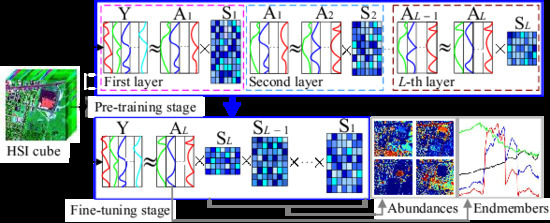
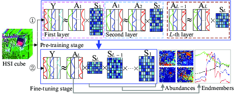
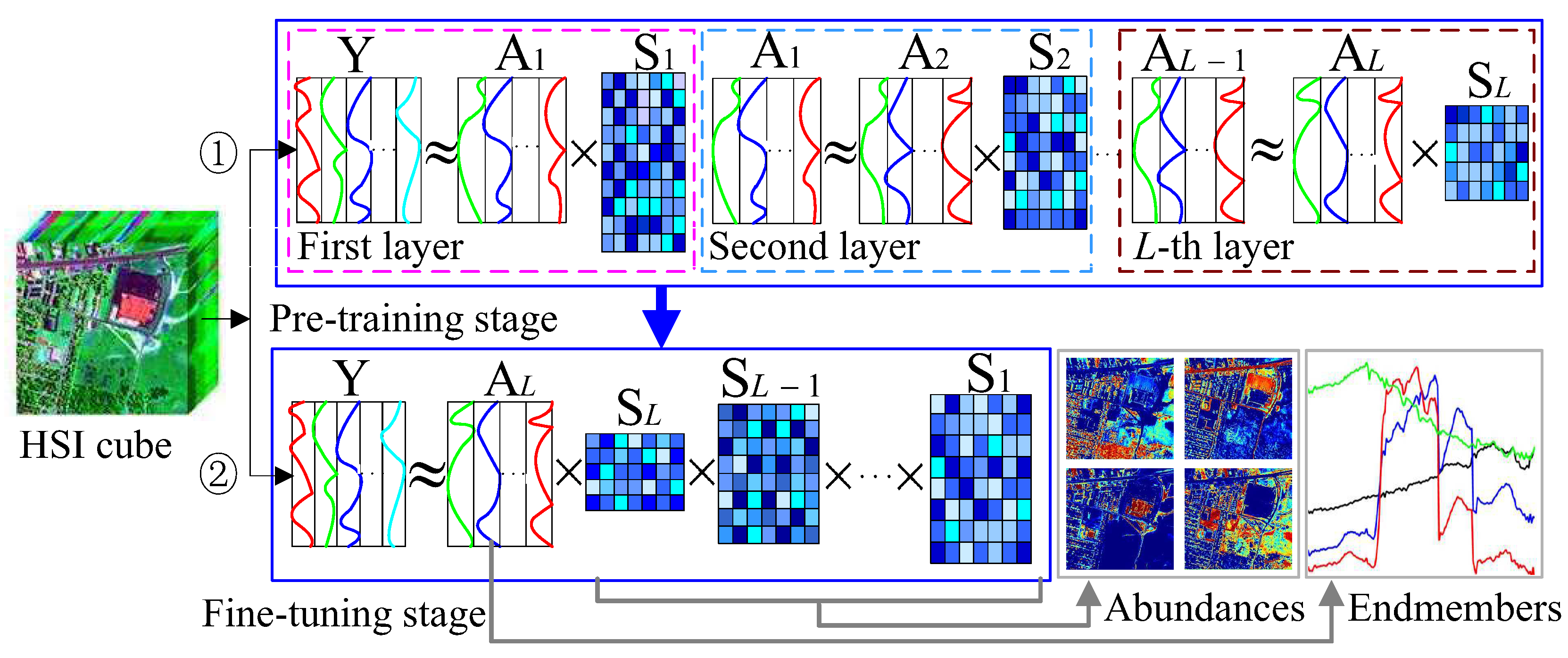
  • We propose a novel Deep Nonnegative Dictionary Factorization method for hyperspectral unmixing. By decomposing the learned dictionary layer by layer in our method, the multi-layer structured representation information implied in HSIs is expected to be captured and used to more accurately extract the target endmembers.
  • Our method incorporates L 1 / 2 sparse constraint and self-supervised regularization into the deep factorization framework, by which the abundance sparseness prior, the sparsity-representation property of dictionaries, as well as the endmember signatures information presented in the data are jointly exploited to guide the unmixing.
  • Our method consists of two stages, where the pre-training stage is designed to decompose the learned basis matrix layer by layer, and the fine-tuning stage are implemented to further optimize all the matrix factors obtained in the previous stage by reconstructing the original data via the production of these factors. Consequently, a set of dictionaries that capture the hierarchical representation relationship of the data are learned in a deep learning way.

2. Related Work

Here we briefly review HU methods based on constrained NMF and deep NMF. Then, the differences between our method and the existing methods are highlighted.
NMF has been demonstrated to be a promising method for HU under the linear spectral mixture model (LMM) [6]. It can decompose a nonnegative HSI matrix into a production of nonnegative endmember and abundance matrices, such that each pixel in an HSI can be represented as a linear combination of endmember spectra in the endmember matrix weighted by its fractional abundances in the abundance matrix [20]. This makes NMF not only possible to simultaneously unmix the endmembers and the corresponding abundances, but also ensure the nonnegativity of the estimated endmembers and abundances, and thus the unmixing results have good interpretability [12]. However, the basic NMF is easy to get into local minima, and also suffers from the problem of non-unique solution [21].
In order to enhance the performance of basic NMF for HU, many improvements have been conducted by developing effective regularizations for NMF, such as the geometry-based regularization and sparseness-based regularization. For example, minimum volume constrained NMF (MVCNMF) [22] is developed by introducing geometry-based regularization in attempt to minimize the volume of the simplex formed by the candidate endmembers. Aiming at exploiting the sparse prior of abundance, L 1 / 2 sparsity-constrained NMF ( L 1 / 2 -NMF) [20] is proposed by employing an effective L 1 / 2 regularizer. On this basis, graph regularized L 1 / 2 -NMF (GLNMF) [23] introduces a graph structure-based regularization that can leverage the intrinsic manifold structure of HSIs. Recently, spatial group sparsity regularized NMF (SGSNMF) is presented by utilizing a spatial group-structured prior information of HSIs [24]. Although existing works have improved the performance of NMF-based unmixing methods, these methods only adopt the single layer factorization, which is not favorable for efficiently utilizing the multi-layers structured information implied in HSIs [17].
Recently, deep NMF-based methods have shown their potentials for unmixing [19,25,26]. The advantages of deep NMF lie in that unlike the single layer NMF decomposes the original data into the production of two matrix factors, it learns the hierarchical and abstract features of the original data by factorizing the coefficient matrix layer by layer [16]. As a result, more complex abstract features from data can be captured and used to improve unmixing performance [19]. However, the existing deep NMF-based unmixing methods mainly focus on factorizing the coefficient matrix neglecting to capture the multi-layer representation relationship among basis matrices.
Unlike these methods, we propose the two-stage deep dictionary factorization to effectively exploit the hierarchical representation relationship of dictionaries in a deep learning way, and design effective regularizations for the hyperspectral unmixing purpose, by which the multi-layers structured information included in HSIs, the abundance sparsity property of data, as well as the endmember signatures information implied in the data are expected to be jointly utilized to more accurately estimate the endmembers and abundances.

3. Methodology

3.1. Notation and Problem Definition

In this paper, we use boldface uppercase letters to represent matrices, and boldface lowercase letters to denote the vectors. For a matrix X R m × n , X denotes the transpose of X , boldface lowercase x n stands for the n-th column vector of X , and [ X ] m n represents the entry of X in the m-th row and n-th column. We use X F to denote the Frobenius norm of X . X 0 signifies that each entry of X is equal to or larger than zero. For l N , we use I l to denote the l × l identity matrix, and 1 l to represent an all-one l × l matrix. The symbol and are used to represent the element-wise multiplication and division operation of the matrix, respectively.
Logically, an HSI can be regarded as an image cube X R M × C × B , where B denotes the number of bands involved in each pixel, whilst M and C denote the number of rows and columns of pixels, respectively. For the sake of computational convenience, this cube can be represented in a matrix form as Y = [ y 1 , y 2 , , y N ] , where Y R B × N , N = M × C , and y n R B denotes the n-th pixel spectrum. According to LMM, given that Y is known, the HU problem can be solved from the perspective of blind source separation, by which Y is approximately reconstructed by Y A S , where A = [ a 1 , a 2 , , a K ] R B × K is the nonnegative endmember matrix with each column a k denoting an endmember; S = [ s 1 , s 2 , , s N ] R K × N represents the nonnegative abundance matrix with s n = ( s n 1 , s n 2 , , s n K ) standing for the abundance vector of the pixel spectrum y n . In other words, we need to estimate both A and S given that only Y is known in actual HU applications.

3.2. DNDF Model

The unmixing performance of constrained NMF-based methods is limited by their single layer factorization ability. Although the existing deep NMF-based unmixing methods have overcome this issue to some extend by decomposing the coefficient matrix in succession, this manner of factorization is unfavorable to exploit the complex multi-layer representation relationship between the endmembers and the mixed pixels included in HSIs. To deal with this challenge, the proposed DNDF model decomposes the basis matrix layer by layer instead of the coefficient matrix. Specifically, the data matrix Y is first factorized into A 1 and S 1 , then A 1 is further decomposed into A 2 and S 2 , next the factorization procedure is continued until the L-th layer is reached. This can be formally expressed as
Y A 1 S 1 , A 1 A 2 S 2 , , A l 1 A l S l , , A L 1 A L S L .
where A l and S l respectively represents the basis and coefficient matrices in the l-th layer. Based on this multi-layer factorization schema, the data matrix Y can be approximately reconstructed by
Y A L S L S L 1 S 1 ,
where A L is regarded as the endmember matrix, and S L S L 1 S 1 is used to generate the abundances.
As shown in Figure 1, our proposed DNDF unmixing model consists of two parts: pre-training model and fine-tuning model. By the pre-training model, we aim to learn multi-layer dictionaries by decomposing the basis matrix layer by layer, so that the endmembers can be better learned from the dictionaries extracted from the HSI data in a deep leaning fashion. With the guidance of fine-tuning model, the obtained matrix factors by the previous model are expected to be optimized jointly by reconstructing the original data as far as possible. Formally, the objective functions of the pre-training Q p and fine-tuning Q f can be respectively expressed as follows:
min A l , S l Q p ( A l , S l ) = A l 1 A l S l F 2 + λ A l E l F 2 k = 1 K l A ¯ l k E ¯ l k F 2 + β S l 1 2 , s . t . A l , S l 0
min A L , S L , , S 1 Q f ( A L , S L , , S 1 ) = Y A L l = L 1 S l F 2 + λ A L E L F 2 k = 1 K L A ¯ L k E ¯ L k F 2 + β l = 1 L S l 1 2 , s . t . A L , S L , , S 1 0
where Y denotes the known HSI matrix; A l 1 is the basis matrix of the ( l 1 ) -th layer and A l 1 = Y in case of l = 1 , while A l and S l represent the basis and coefficient matrix of the l-th layer, respectively; λ and β are regularization parameters. Specifically, the first term in Q p plays the same role of single layer NMF for decomposing the dictionary A l 1 , whereas the function of first term in Q f is to reconstruct Y using the product of the matrix factors learned based on Q p . The second and third terms in both Q p and Q f are the self-supervised regularization and sparseness regularization, respectively. Since weakly supervised information for the basis matrix helps improve the performance of NMF [27], we employ the self-supervised fashion to learn effective weakly supervised information as guidance for extracting accurate endmembers. Specifically, before each factorization in the layer l, where l = 1 , 2 , , L , the Fuzzy C-means (FCM) clustering method is conducted on Y , then the obtained cluster centers are used to construct the approximate endmember matrix E l , which functions as the weakly supervised information for the endmember matrix. Note that the number of clusters of FCM equals the number of column vectors in the basis matrix of the l-th layer; E l = [ e 1 , e 2 , , e K l ] denotes the approximate endmember matrix with each e k , k = 1 , 2 , , K l representing a clustering center given by FCM, whereas A ¯ k and E ¯ k are respectively defined by
A ¯ l k = [ a k , a k , , a k ] K l 1 and E ¯ l k = [ e 1 , e 2 , , e k 1 , e k + 1 , , e K l ] .
It is worth pointing out that the numerator of proposed self-supervised regularization term plays the role of keeping the achieved A l as similar as the approximate endmember matrix E l whilst the denominator aims to make each estimated endmember a k has the maximum difference with the other clustering centers except for e k .
To learn a sparse representation between dictionaries, sparsity constraint is also imposed on the coefficient matrix in the factorization of each layer. The effectiveness of this measures lies in that the sparsity of abundance distribution is an intrinsic property of HSIs [20,23,24], as well as sparse representation enforces the learned endmember signatures to be more similar to the real endmember. Previous studies have demonstrated that L 1 / 2 regularization has the superiority for enforcing the sparseness of decomposed abundance matrix. Thus, the L 1 / 2 regularizer S 1 2 = i , j ( s i , j ) 1 2 is introduced into Q p and Q f to impose sparsity constraint on the S l .

3.3. Optimization and Implementation

Since the objective functions in Equations (3) and (4) are both non-convex w.r.t two or more matrix factors simultaneously, we deduce the multiplicative update rules (MURs) of the proposed unmixing model by alternating optimization, by which each matrix factor is updated with the others being fixed.
(i) MURs for the pre-training stage. Considering the objective function Q p in Equation (3), when A l remains unchanged, the MUR of S via [20] can be given as follows:
S l S l A l A l 1 ( ( A l A l ) S l + β ( S l ) 1 2 ) ,
where [ ( S l ) 1 2 ] i j = [ S l ] i j 1 2 . As for the MUR of A l , we first give the gradient of function Q p w.r.t A l by
Q p A l = A l S l S l A l 1 S l λ G ( A l , E l ) + λ H ( A l , E l ) ,
where matrix W = 1 K l I K l ; The functions G and H are respectively defined by
G ( A l , E l ) = E l ( k = 1 K l A ¯ l k E ¯ l k F 2 + A l E l F 2 W ) ( k = 1 K l A ¯ l k E ¯ l k F 2 ) 2 ,
H ( A l , E l ) = ( k = 1 K l A ¯ l k E ¯ l k F 2 + ( K l 1 ) A l E l F 2 ) A l ( k = 1 K l A ¯ l k E ¯ l k F 2 ) 2 .
Based on the gradient descent principle, the update rule for A l can be given by
[ A l ] m i [ A l ] m i η m i Q p [ A l ] m i .
Then, we set η m i = A l ( A l S l S l + λ H ( A l , E l ) ) in Equation (6). The MUR for A l can be deduced as
A l A l ( A l 1 S l + λ G ( A l , E l ) ) ( A l S l S l + λ H ( A l , E l ) ) .
(ii) MURs for the fine-tuning stage. For the objective function Q f in Equation (4), when S L , , S 1 keep fixed and are regarded as a whole matrix, the MUR of A L can be obtained in terms of the deduction procedure of MUR in Equation (7). It can be expressed as
A L A L ( Y ( l = L 1 S l ) + λ G ( A L , E L ) ) ( A L ( l = L 1 S l ) l = L 1 S l + λ H ( A L , E L ) ) .
Similarly, when A L S L S L 1 S 2 is considered as a fixed matrix, the MUR of S 1 can be given as
S 1 S 1 ( A L l = L 2 S l ) Y ( ( A L l = L 2 S l ) ( A L l = L 2 S l ) S 1 + β ( S 1 ) 1 2 ) ,
For the derivation of the MUR of S l ,where l = 2 , 3 , , L , Q f in Equation (4) can be re-expressed as
Q f ( S l ) = 1 2 Y Φ S l Ψ F 2 + λ 2 A L E L F 2 k = 1 K L A ¯ L k E ¯ L k F 2 + β l = 1 L S l 1 2 ,
where Φ = A L S L S l + 1 and Ψ = S l 1 S 1 , respectively. The additive update for S l can be given as
[ S l ] u v [ S l ] u v η u v Q d [ S l ] u v .
The gradient of Q f w.r.t S l can be expressed by
Q f [ S l ] u v = Φ Y Ψ + Φ Φ S l Ψ Ψ + λ 2 S l 1 2 .
By substituting Equation (12) into Equation (11) and setting η u v = S l ( Φ Φ S l Ψ Ψ + λ S l 1 2 ) , the MUR of S l can be derived as
S l S l ( Φ Y Ψ ) ( Φ Φ S l Ψ Ψ + λ S l 1 2 ) .
Based on the above analysis, the pseudo-code of the proposed DNDF algorithm for HU is summarized in Algorithm 1. It mainly consists of two parts: the pre-training part (Line 2–10) and the fine-tuning part (Line 12–18). For the pre-training part, it is worth noting that A l is initialized based on the cluster centers given by the FCM method, while the initial values of S l are provided by the fully constrained least squares algorithm [28].
Algorithm 1: DNDF Algorithm For HU
Remotesensing 12 02882 i001

4. Experiment

Here, we first briefly introduce the datasets used in the experiments, the baseline methods and algorithm settings, as well as the performance metrics. Then, the quantitative evaluation, factors exploration and parameter analysis are addressed.

4.1. Experiment Setting

Datasets.Table 1 summarizes the statistics of three real datasets used in the experiments and Figure 2 shows their visual pseudo-color images. (1) Samson comprises 952 × 952 pixels and has 156 bands covering the wavelengths from 0.401 to 0.889 μ m. For computational convenience, a subimage that has the size of 95 × 95 pixels and contains three types of endmembers (Soil, Tree, and Water) is chosen from the original data and used in the experiment [19,29]. (2) Jasper Ridge was collected by the Airborne Visible/Infrared Imaging Spectrometer (AVIRIS) sensor. The original data has 512 × 614 pixels, each of which is recorded with 224 bands with the wavelength ranging from 0.380 to 2.5 μ m. Following the setting of [30], a subimage with 100 × 100 pixels is adopted. The target scene mainly has four kinds of endmebers: Soil, Water, Road, and Tree. To eliminate the impact of the dense water vapor and atmospheric effects, the spectral bands 1–3, 108–112, 154–166 and 220–224 are removed from the data, leaving 198 bands. (3) Washington DC Mall is captured by the airborne HYperspectral Digital Imagery Collection Experiment (HYDICE) sensor over the Washington DC Mall area, USA. The original data consists of 210 spectral bands with wavelengths from 0.4 to 2.5 μ m. A subimage with 150 × 150 pixels from the original HSI is used in the experiment [31]. There are five types of endmembers in the selected subimage including Grass, Tree, Street, Roof, and Water. We deleted the bands corrupted by noise seriously, as well as the water vapor absorption bands (including bands 103–106, 138–148 and 207–210) from the data and the remaining 191 bands were used.
Baseline Methods. We compare the proposed DNDF with four kinds of NMF-based unmixing methods. (1) Two sparsity-constrained NMF-based algorithms such as L 1 / 2 -NMF [20] and SGSNMF [24]; (2) An NMF-based method with spectral geometry related constrain, i.e., MVCNMF [22]; (3) A representative graph-regularization based NMF, named GLNMF [23]; (4) A state-of-the-art deep NMF-based unmixing approach, i.e. deep NMF with total variation (SDNMF-TV) [19]. The algorithm parameters for all baseline methods adopt the same values as those in their original works. To make a fair comparison, all the algorithms initialize the endmember and abundance matrics by vertex component analysis (VCA) [32] and FCLS [28], respectively, except for SGSNMF, which initializes the endmember matrix with the help of superpixel segmentation. Additionally, we test our method under the condition that the number of factorization layers is set to 1 and 2, respectively, and the obtained algorithms are referred to as DNDF-L1 and DNDF-L2 accordingly. The maximum number of iterations is set to 500 for pre-training, and 4000 for the fine-tuning stage. We set the experience values of regularization parameters to λ = 0.1 and β = 0.1 , respectively. All the algorithms are tested 20 times and the average performance is reported.
Performance Metrics. To evaluate the performance of our method, Spectral Angle Distance (SAD) [19,20], which can measure the similarity between an estimated endmember and the reference one, is adopted. Given that a ^ k and a k respectively denote the estimated and the reference endmember, SAD can be defined as
SAD ( a k , a ^ k ) = arccos a k a ^ k a k a ^ k ,
where · denotes the Euclidean norm of vectors. Since SAD represents the angular distance between two vectors, a smaller SAD value indicates better performance. According to its definition, the SAD measure has the unit of “radians”.

4.2. Performance Evaluation

To test the performance of our method, three experiments are conducted on different datasets. The performance evaluation is presented from three aspects: quantitative evaluation, factor exploration, and algorithm parameter analysis.
Quantitative Evaluation. The quantitative comparisons about the experimental results on three datasets are reported in Table 2 including the SAD values of each endmember and their averages of all the endmembers provided by each baseline algorithm. Each row corresponding to the individual endmember shows the performance of all methods w.r.t this endmember, whereas the rows indicated by “Average” denote the average SAD values of all the endmembers of a specific dataset. The value with red color denotes the best performance, whilst the blue value indicates the second best. As can be seen from the average SAD respectively, the proposed DNMF-L2 performs best on all three datasets. It reduces 9.9 % mean SAD on the Samson dataset compared with the second best method, i.e., DNMF-L1. According to the results on the Jasper Ridge and Washington DC Mall datasets, DNMF-L2 decreases the mean SAD of 9.7 % and 8.6 % respectively than the second best method, i.e., GLNMF. As for the performance on individual endmember, DNDF-L2 has the largest number of second-best instances on Samson, and provides a best and a second best instances among four endmembers on Jasper Ridge. On Washington DC Mall, DNDF-L2 shows its superiority by giving one best and two second best instances within five endmembers.
Factor Exploration. To provide an intuitive evaluation about DNDF, we provide some visual results. Figure 3 shows an example of the learned hierarchical dictionaries on the Samon by the obtained basis matrices A 1 and A 2 in the pre-training stage of DNDF-L2. The atoms of the dictionary learned by the factorization of first layer are respectively plotted in Figure 3a–c according to their categories, whereas Figure 3d–f show the atoms of dictionary of the second layer. Here, the red solid lines denote the reference endmember signatures while the dotted lines represent the atoms. As can be seen in Figure 3a–c, the learned atoms have good similarity to the reference signatures except for a particular learned signature with yellow color in Figure 3c. It also can be seen from Figure 3d–f, the learned atoms have good consistency with the corresponding reference signatures, revealing the effectiveness of our method. In order to qualitatively interpret the abundance estimations, we illustrate some instances of the abundance maps unmixed by all the methods in Figure 4. All the abundance maps are represented by a heatmap manner, where the pixel with high color temperature denotes a big presence proportion of corresponding endmember.
Next, we investigate the effectiveness of each term in our proposed model. Table 3 shows the performance comparison of on three datasets, where DNDF denotes the proposed method without any regularization, DNDF-SP, DNDF-SS, and DNDF-L2 represent the proposed method with sparse regularization, self-supervised regularization and both regularizations, respectively. We can see that the integrated model outperforms the partial components, which demonstrates the effectiveness of the joint work of different terms.
Parameter Analysis. Here, we analyze the impact of two algorithm parameters. We first fix β = 0.1 , then choose different values for λ from the set { 1 × 10 4 , 1 × 10 3 , 0.01 , 0.1 , 0.2 , 0.3 , 0.4 , 0.5 } . Figure 5a shows the performance of DNDF-L2 on Jasper Ridge dataset. As can be seen, the performance our algorithm ascends in the first steps gets better SAD values when λ [ 0.01 , 0.2 ] , and the performance degrades when λ 0.3 . λ = 0.1 is the optimal selection according to SAD criteria. Next, the impact of β on our algorithm is tested on the condition that λ is fixed to 0.1, whilst selecting different values for β in the same collection as λ . As Figure 5b shows that our algorithm has better performance when β [ 0.01 , 0.3 ] , and β = 0.1 is the best choice.
Running Time. To evaluate the performance of our methods on running time, we tested all the seven methods on three datasets. The average running time of them are reported in Table 4. From Table 4, it can be seen that DNDF-L2 needs shorter time than SDNMF-TV and MVCNMF on all the the datasets. According to the results on the Samson dataset, we can see from Table 4 that the running time of DNDF-L1 is the least, and SDNMF-TV needs the most time. When all the methods are tested on Jasper Ridge dataset, L 1 / 2 -NMF consumes the least time, followed by DNDF-L1. As to the results on Wash. DC Mall dataset, L 1 / 2 -NMF performs best, and DNDF-L1 is better than SGSNMF, DNDF-L2, SDNMF-TV, and MVCNMF.

5. Conclusions

We proposed a novel Deep Nonnegative Dictionary Factorization framework with L 1 / 2 sparseness constraint and self-supervised regularization for hyperspectral unmixing task, which integrated the pre-training stage and fine-tuning stage into a unified model. By imposing sparse constraints on the coefficient matrices, DNDF jointly exploited the sparseness prior of abundance, as well as the sparsity-representation property of dictionaries. In addition, the self-supervised regularization based on the guidance of fuzzy clustering helped to learn hierarchical dictionaries that captured the latent endmembers. Experiments conducted on three real-world datasets demonstrated the effectiveness and superiority of our approach compared with several state-of-the-art methods based on single-layer NMF and deep NMF.

Author Contributions

Conceptualization, W.W. and H.L.; Data curation, W.W.; Formal analysis, W.W.; Funding acquisition, W.W.; Investigation, W.W.; Methodology, W.W.; Project administration, H.L.; Resources, H.L.; Software, W.W.; Supervision, H.L.; Validation, W.W.; Visualization, W.W.; Writing—original draft, W.W.; Writing—review & editing, W.W. and H.L. All authors have read and agreed to the published version of the manuscript.

Funding

This research was funded by the project ZR2017MF028 supported by Shandong Provincial Natural Science Foundation.

Acknowledgments

We would like to thank Yanfei Zhong (State Key Laboratory of Information Engineering in Surveying, Mapping and Remote Sensing, Wuhan University, Wuhan, China) and Hairong Qi (Department of Electrical Engineering and Computer Science, University of Tennessee, Knoxville, TN, USA) for sharing the source codes.

Conflicts of Interest

The authors declare no conflict of interest.

Abbreviations

The following abbreviations are used in this manuscript:
HSIHyperspectral remote sensing image
HUHyperspectral unmixing
NMFNonnegative matrix factorization
DNDFDeep nonnegative dictionary factorization
VCAVertex component analysis
FCLSFully constrained least squares
LMMLinear spectrum mixture model
SADSpectral angle distance
RMSERoot mean square error
MURMultiplicative update rule

References

  1. Nalepa, J.; Myller, M.; Kawulok, M. Validating Hyperspectral Image Segmentation. IEEE Geosci. Remote Sens. Lett. 2019, 16, 1264–1268. [Google Scholar] [CrossRef] [Green Version]
  2. He, N.; Paoletti, M.E.; Haut, J.M.; Fang, L.; Li, S.; Plaza, A.; Plaza, J. Feature Extraction With Multiscale Covariance Maps for Hyperspectral Image Classification. IEEE Trans. Geosci. Remote Sens. 2019, 57, 755–769. [Google Scholar] [CrossRef]
  3. Zhang, W.; Lu, X.; Li, X. Similarity Constrained Convex Nonnegative Matrix Factorization for Hyperspectral Anomaly Detection. IEEE Trans. Geosci. Remote Sens. 2019, 57, 4810–4822. [Google Scholar] [CrossRef]
  4. Xiong, F.; Zhou, J.; Qian, Y. Material Based Object Tracking in Hyperspectral Videos. IEEE Trans. Image Process. 2020, 29, 3719–3733. [Google Scholar] [CrossRef]
  5. Chen, Q.; Sun, J.; Palade, V.; Shi, X.; Liu, L. Hierarchical Clustering Based Band Selection Algorithm for Hyperspectral Face Recognition. IEEE Access 2019, 7, 24333–24342. [Google Scholar] [CrossRef]
  6. Bioucas-Dias, J.M.; Plaza, A.; Dobigeon, N.; Parente, M.; Du, Q.; Gader, P.; Chanussot, J. Hyperspectral Unmixing Overview: Geometrical, Statistical, and Sparse Regression-Based Approaches. IEEE J. Sel. Top. Appl. Earth Obs. Remote Sens. 2012, 5, 354–379. [Google Scholar] [CrossRef] [Green Version]
  7. Wang, N.; Du, B.; Zhang, L. An Endmember Dissimilarity Constrained Non-Negative Matrix Factorization Method for Hyperspectral Unmixing. IEEE J. Sel. Top. Appl. Earth Obs. Remote Sens. 2013, 6, 554–569. [Google Scholar] [CrossRef]
  8. Zare, A.; Ho, K.C. Endmember Variability in Hyperspectral Analysis: Addressing Spectral Variability During Spectral Unmixing. IEEE Signal Process. Mag. 2014, 31, 95–104. [Google Scholar] [CrossRef]
  9. Lee, D.D.; Seung, H.S. Learning the parts of objects by non-negative matrix factorization. Nature 1999, 401, 788–791. [Google Scholar] [CrossRef]
  10. Lee, D.D.; Seung, H.S. Algorithms for Non-negative Matrix Factorization. In Advances in Neural Information Processing Systems; Leen, T.K., Dietterich, T.G., Tresp, V., Eds.; MIT Press: Cambridge, MA, USA, 2001; pp. 556–562. [Google Scholar]
  11. Cai, D.; He, X.; Han, J.; Huang, T.S. Graph Regularized Nonnegative Matrix Factorization for Data Representation. IEEE Trans. Pattern Anal. Mach. Intell. 2011, 33, 1548–1560. [Google Scholar]
  12. Wang, W.; Qian, Y. Adaptive L1/2 Sparsity-Constrained NMF With Half-Thresholding Algorithm for Hyperspectral Unmixing. IEEE J. Sel. Top. Appl. Earth Obs. Remote Sens. 2015, 8, 2618–2631. [Google Scholar] [CrossRef]
  13. Lu, Y.; Yuan, C.; Zhu, W.; Li, X. Structurally Incoherent Low-Rank Nonnegative Matrix Factorization for Image Classification. IEEE Trans. Image Process. 2018, 27, 5248–5260. [Google Scholar] [CrossRef]
  14. Yang, Z.; Xiang, Y.; Xie, K.; Lai, Y. Adaptive Method for Nonsmooth Nonnegative Matrix Factorization. IEEE Trans. Neural Net. Learn. Syst. 2017, 28, 948–960. [Google Scholar] [CrossRef]
  15. Li, J.; Li, Y.; Song, R.; Mei, S.; Du, Q. Local Spectral Similarity Preserving Regularized Robust Sparse Hyperspectral Unmixing. IEEE Trans. Geosci. Remote Sens. 2019, 57, 7756–7769. [Google Scholar] [CrossRef]
  16. Trigeorgis, G.; Bousmalis, K.; Zafeiriou, S.; Schuller, B.W. A Deep Matrix Factorization Method for Learning Attribute Representations. IEEE Trans. Pattern Anal. Mach. Intell. 2017, 39, 417–429. [Google Scholar] [CrossRef] [Green Version]
  17. Meng, Y.; Shang, R.; Shang, F.; Jiao, L.; Yang, S.; Stolkin, R. Semi-Supervised Graph Regularized Deep NMF With Bi-Orthogonal Constraints for Data Representation. IEEE Trans. Neural Net. Learn. Syst. 2019, 31, 3245–3258. [Google Scholar] [CrossRef]
  18. Zhang, Z.; Wang, Q.; Yuan, Y. Hyperspectral Unmixing VIA L1/4 Sparsity-Constrained Multilayer NMF. In Proceedings of the 2019 IEEE International Geoscience and Remote Sensing Symposium, Yokohama, Japan, 28 July–2 August 2019; pp. 2143–2146. [Google Scholar]
  19. Feng, X.; Li, H.; Li, J.; Du, Q.; Plaza, A.; Emery, W.J. Hyperspectral Unmixing Using Sparsity-Constrained Deep Nonnegative Matrix Factorization With Total Variation. IEEE Trans. Geosci. Remote Sens. 2018, 56, 6245–6257. [Google Scholar] [CrossRef]
  20. Qian, Y.; Jia, S.; Zhou, J.; Robles-Kelly, A. Hyperspectral Unmixing via L1/2 Sparsity-Constrained Nonnegative Matrix Factorization. IEEE Trans. Geosci. Remote Sens. 2011, 49, 4282–4297. [Google Scholar] [CrossRef] [Green Version]
  21. Wang, Y.; Zhang, Y. Nonnegative Matrix Factorization: A Comprehensive Review. IEEE Trans. Knowl. Data Eng. 2013, 25, 1336–1353. [Google Scholar] [CrossRef]
  22. Miao, L.; Qi, H. Endmember Extraction From Highly Mixed Data Using Minimum Volume Constrained Nonnegative Matrix Factorization. IEEE Trans. Geosci. Remote Sens. 2007, 45, 765–777. [Google Scholar] [CrossRef]
  23. Lu, X.; Wu, H.; Yuan, Y.; Yan, P.; Li, X. Manifold Regularized Sparse NMF for Hyperspectral Unmixing. IEEE Trans. Geosci. Remote Sens. 2013, 51, 2815–2826. [Google Scholar] [CrossRef]
  24. Wang, X.; Zhong, Y.; Zhang, L.; Xu, Y. Spatial Group Sparsity Regularized Nonnegative Matrix Factorization for Hyperspectral Unmixing. IEEE Trans. Geosci. Remote Sens. 2017, 55, 6287–6304. [Google Scholar] [CrossRef]
  25. Rajabi, R.; Ghassemian, H. Spectral Unmixing of Hyperspectral Imagery Using Multilayer NMF. IEEE Geosci. Remote Sens. Lett. 2015, 12, 38. [Google Scholar] [CrossRef] [Green Version]
  26. Fang, H.; Li, A.; Wang, T.; Xu, H. Hyperspectral unmixing using double-constrained multilayer NMF. Remote Sens. Lett. 2019, 10, 224–233. [Google Scholar] [CrossRef]
  27. Choo, J.; Lee, C.; Reddy, C.K.; Park, H. Weakly supervised nonnegative matrix factorization for user-driven clustering. Data Min. Knowl. Disc. 2015, 29, 1598–1621. [Google Scholar] [CrossRef]
  28. Heinz, D.C.; Chang, C.I. Fully constrained least squares linear spectral mixture analysis method for material quantification in hyperspectral imagery. IEEE Trans. Geosci. Remote Sens. 2001, 39, 529–545. [Google Scholar] [CrossRef] [Green Version]
  29. Zhu, F.; Wang, Y.; Fan, B.; Xiang, S.; Meng, G.; Pan, C. Spectral Unmixing via Data-Guided Sparsity. IEEE Trans. Image Process. 2014, 23, 5412–5427. [Google Scholar] [CrossRef] [Green Version]
  30. Zhu, F. Hyperspectral Unmixing: Ground Truth Labeling, Datasets, Benchmark Performances and Survey. arXiv 2017, arXiv:1708.05125. [Google Scholar]
  31. Jia, S.; Qian, Y. Constrained Nonnegative Matrix Factorization for Hyperspectral Unmixing. IEEE Trans. Geosci. Remote Sens. 2009, 47, 161–173. [Google Scholar] [CrossRef]
  32. Nascimento, J.M.P.; Bioucas-Dias, J.M. Vertex component analysis: A fast algorithm to unmix hyperspectral data. IEEE Trans. Geosci. Remote Sens. 2005, 43, 898–910. [Google Scholar] [CrossRef]
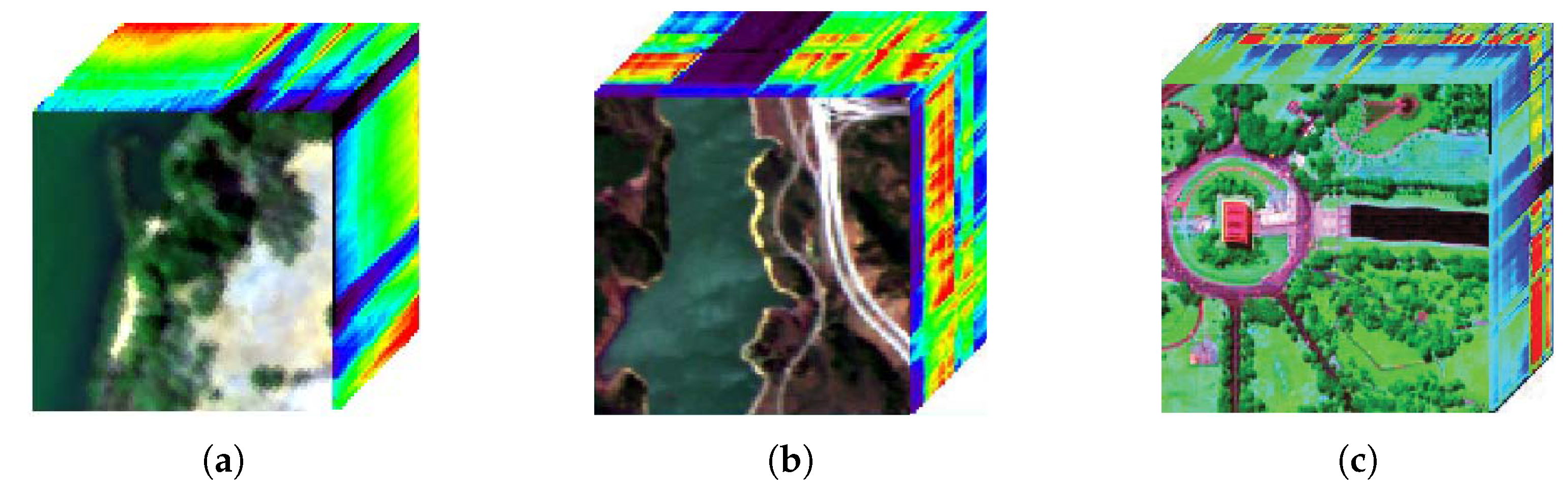
 [Green Version]
Figure 1. Illustration of the proposed model of deep nonnegative dictionary factorization that includes two parts: pre-training and fine-tuning stages. By the pre-training stage, we aim to learn a set of dictionaries A 1 , , A L with hierarchical representation relationship by decomposing the basis matrix layer by layer, so that endmembers can be better learned from the dictionaries extracted from the HSI data in a deep leaning fashion. With the guidance of fine-tuning model, the obtained matrix factors A L , S L , , S 1 in the previous stage are expected to be further optimized jointly by reconstructing the HSI matrix Y as far as possible.
Remotesensing 12 02882 g001
Figure 2. Pseudo-Color images of three real hyperspectral image datasets. (a) Samson; (b) Jasper Ridge; (c) Wash. DC Mall.
Remotesensing 12 02882 g002
Figure 3. Comparison between the reference endmembers (red solid line) and the atoms (dotted line) of the learned dictionaries given by our DNDF-L2 on Samson. (ac) plots the reference endmembers and the atoms of the dictionary learned in the first layer factorization, and (df) compares the reference endmembers and the atoms of the dictionary of second layer. (a) Soil; (b) Tree; (c) Water; (d) Soil; (e) Tree; (f) Water.
Remotesensing 12 02882 g003
Figure 4. Abundance maps estimated by DNDF-L1, DNDF-L2, GLNMF, SDNMF-TV, SGSNMF, MVCNMF, L 1 / 2 -NMF on Washington DC Mall. (a) Grass; (b) Tree; (c) Roof; (d) Street; (e) Water.
Remotesensing 12 02882 g004
Figure 5. Algorithm parameter analysis on Jasper Ridge. (a) Parameter λ ; (b) Parameter β .
Remotesensing 12 02882 g005
Table 1. Characteristics of three real hyperspectral image datasets
Dataset# Endmember# Band# PixelWavelengthSensor-Type
Samson3156 95 × 95 0.401–0.889 μ mSAMSON
Jasper Ridge4198 100 × 100 0.38–2.5 μ mAVIRIS
Wash. DC Mall5191 150 × 150 0.4–2.5 μ mHYDICE
# means the number of something. # Band means the number of band.
Table 2. Performance comparison w.r.t the metric of spectral angle distance (SAD) on three datasets (in radians), where a smaller SAD value indicates better performance signifying the better similarity between the estimated endmember and the reference one. Red bold and blue italic denote the best and second-best results, respectively.
SamsonDNDF-L1DNDF-L2GLNMFSDNMF-TVSGSNMFMVCNMF L 1 / 2 -NMF
Soil0.02200.01600.02750.17610.00970.31480.0279
Tree0.02900.03160.04230.13100.04590.07340.0426
Water0.17580.15670.22940.09220.22890.32040.3015
Average0.07560.06810.09970.13310.09490.23650.1240
Jasper RidgeDNDF-L1DNDF-L2GLNMFSDNMF-TVSGSNMFMVCNMF L 1 / 2 -NMF
Tree0.06090.07290.12700.10260.14150.17520.1187
Water0.06940.06590.18720.10880.22360.29800.2022
Soil0.11730.20100.11700.10690.13850.14060.1324
Road0.37540.11230.06970.46620.04830.14580.0690
Average0.15580.11300.12520.19610.13800.18990.1306
Wash. DC MallDNDF-L1DNDF-L2GLNMFSDNMF-TVSGSNMFMVCNMF L 1 / 2 -NMF
Tree0.00950.03210.17380.09930.16060.23720.1738
Grass0.11280.14040.25850.16820.14250.25710.2688
Street0.70730.52930.38870.45200.69630.58590.4195
Roof0.24350.26320.19420.36450.25250.16630.1720
Water0.07530.04620.09200.25090.10010.11170.0892
Average0.22970.20230.22140.26700.27040.27160.2247
Table 3. Performance comparison w.r.t the SAD values on three datasets (in radians), where DNDF denotes the proposed method without any regularization, DNDF-SP, DNDF-SS, and DNDF-L2 represent the proposed method with sparse regularization, self- supervised regularization and both regularizations, respectively. Red bold and blue italic denote the best and second-best results, respectively.
SamsonDNDFDNDF-SPDNDF-SSDNDF-L2
Soil0.01690.01650.01640.0160
Tree0.03250.03190.03210.0316
Water0.16720.16350.16100.1567
Average0.07220.07060.06980.0681
Jasper RidgeDNDFDNDF-SPDNDF-SSDNDF-L2
Tree0.07720.07420.07350.0729
Water0.06860.06210.06660.0659
Soil0.19790.20660.17640.2010
Road0.14810.13270.14230.1123
Average0.12300.11890.11470.1130
Wash. DC MallDNDFDNDF-SPDNDF-SSDNDF-L2
Tree0.04270.03390.04470.0321
Grass0.14830.14240.14650.1404
Street0.59580.56860.55700.5293
Roof0.25860.25940.25790.2632
Water0.04780.04560.03840.0462
Average0.21860.21000.20890.2023
Table 4. Running time on three real data sets (in seconds).
Data SetsDNDF-L1DNDF-L2GLNMFSDNMF-TVSGSNMFMVCNMF L 1 / 2 -NMF
Samson 25.77 113.17 48.20 462.18 42.49 262.0442.41
Jasper Ridge 60.82 169.68 64.56 558.40 68.28 583.2454.52
Wash. DC Mall 130.81 385.52 102.13 1062.78 161.88 1229.9189.43

