Nutrient Prediction for Tef (Eragrostis tef) Plant and Grain with Hyperspectral Data and Partial Least Squares Regression: Replicating Methods and Results across Environments

Abstract

Achieving reproducibility and replication (R&R) of scientific results is tantamount for science to progress, and it is also necessary for ensuring the self-correcting mechanism of the scientific method. Topics of R&R have sailed to the forefront of research agenda in many fields recently but have received less attention in remote sensing in general and specifically for studies utilizing hyperspectral data. Given the extremely local environments in which many hyperspectral studies are conducted (e.g., agricultural field plots), purposeful attention to the repeatability of findings across study locales can help ensure methods are generalizable. This study undertakes an investigation of the nutrient content of tef (Eragrostis tef), an understudied plant that is growing in importance due to both food and forage benefits, but does so within the context of the replicability of methods and findings across two study sites situated in different international and environmental contexts. The aims are to (1) determine whether calcium, magnesium, and protein of both the plant and grain can be predicted using hyperspectral data with partial least squares (PLS) regression with waveband selection, and (2) compare the replicability of models across differing environments. Results suggest the method can produce high nutrient prediction accuracy for both the plant and grain in individual environments, but selection of wavebands for nutrient prediction was not comparable across study areas. The findings suggest that the method must be calibrated in each location, thereby reducing the potential to extrapolate methods to different areas. Our findings highlight the need for greater attention to methods and results replication in remote sensing, specifically hyperspectral analyses, in order for scientific findings to be repeatable beyond the plot level.

1. Introduction

The reproducibility and replication (R&R) of scientific findings has recently moved to the forefront of research agenda in many fields [1,2,3,4,5] since it has been discovered that findings often cannot be reproduced or replicated [5,6]. While the two “R’s”—reproducibility and replicability—are intertwined, there are key differences between their goals. Adopting the definitions from the National Science Foundation [7] and the National Academy of Science, Engineering, and Medicine [8], we define reproducibility as the ability of a researcher to duplicate the results of a prior study using the same data and methods as the original investigator. In short, if a researcher makes the data and methods/code available, another researcher should be able to produce the exact same results. In comparison, replicability is the ability of a researcher to duplicate results using similar methods but with new data.

Achieving R&R is critical for advancing scientific discoveries, yet neither topic has received much attention in geography and the spatial sciences, where investigations tend to be observational instead of experimental or theoretical [9]. R&R has received even less attention in remote sensing (but see [10] for an early take), even though the field is uniquely positioned to contribute to R&R on several fronts. First, there is a rich archive of publicly available remote sensing datasets (e.g., Landsat), supporting opportunities for reproducibility [9,11]. Second, remote sensing studies, and in particular hyperspectral studies, are often situated in extremely local contexts (e.g., agricultural plots) due to the need for ground reference data and the high labor and time costs of operating equipment. Yet, an implicit goal of science is to develop widely applicable methodologies and generalizable findings that can be applied in different contexts. Thus, working toward the replicability of methods and findings across different study areas is important for advancing remote sensing science.

Despite the myriad opportunities for remote sensing scientists to explore R&R issues, very few formal efforts have been documented. One reason is likely because remote sensing scientists often work with large datasets and perform complex spectral and spatial manipulations [12,13,14,15,16], which makes R&R difficult if processing code is not made available. Until recently, many scientific publications did not require code to be submitted as part of the manuscript review process, although this is changing. Replication in remote sensing is also hindered by attributes of local environments, which makes the transfer of results from one landscape to another difficult. However, if we are to develop methodologies that are transferrable across space, it is necessary to begin developing and implementing protocols for testing the R&R of remote sensing studies. One way to do this is to incorporate multi-field, multi-environment analyses into studies to self-test the replicability of methods and results.

Precision agriculture is one field where immediate gains can be made toward testing the replicability of methods while also contributing a larger understanding of the extent of R&R issues in remote sensing. Since the overall goal of precision agriculture is to decrease the ambiguity of decisions required on agricultural lands that are often highly variable [17], the ability to transfer methods and findings from one environment or location to another requires them to be replicable [18]. However, most studies capture data in a single region or location (often in a single crop field) under uniform conditions [12,15], thus limiting their generalizability across environmental or geographical contexts. Furthermore, the implicit assumption is that methods and findings are extendable beyond the single field in which they were tested, but in most cases, no such evidence is provided. Many studies lack basic explanation for environmental variances such as soil, hydrology, and topography that can cause reflectance variations, thereby altering results across space [16]. Ultimately, remote sensing methodologies are of little practical value for precision agriculture if they are developed, tested, and applicable in a single location where these multiple and often confounding factors are held constant.

Partial least squares (PLS) regression has become an accepted technique in vegetation studies using hyperspectral data for estimating a range of biophysical and biochemical properties [19,20,21,22,23]. In situations where the number of independent variables is large and the variables are collinear, which is common with hyperspectral data, multiple linear regression will often overfit the model [24,25]. PLS regression standardizes model construction from the preprocessed hyperspectral data via latent variables, from which the predictive capabilities of the model can be tested. Recently, variations of PLS regression using a waveband selection procedure [13] have been proposed and adopted, but there has been little effort to test the replicability of these methods across environments to determine whether results might be transferable.

The objective of this study is to investigate the replicability of PLS regression methods, including PLS with waveband selection, for predicting nutrient content in plant and grain material across multiple environments. This study addresses gaps in the remote sensing R&R literature by replicating a methodological workflow using hyperspectral data and PLS regression for predicting nutrients in a single crop but in two varying environments in different international contexts to determine the degree to which the methods are replicable. The focus is on Eragrostis tef (tef), a cereal crop primarily grown in Ethiopia, although production has been expanding to other parts of the world due to its versatility and resistance to drought. Tef is ideal for studying replicability because it is grown in different international contexts and is known for being successfully cultivated across differing environments. Additionally, very few hyperspectral analyses have been performed on non-milled grains [26], so this study contributes knowledge in that realm as well.

Tef is a grass (Family: Poaceae) that has received little attention from the remote sensing and precision agricultural communities despite its versatile cultivation characteristics. Tef is thought to be one of the earliest domesticated plants [27], with the center of origin and diversity in Ethiopia/Horn of Africa [28]. It is drought and heat resistant, has a high nutrient content, and is grown for animal feed as well as a staple food crop [29]. While tef can be cultivated across many environments, it is primarily grown in Ethiopia, where it is the most commonly harvested crop, popular for its highly nutritious, gluten-free grain [30,31,32,33,34,35]. Recently, cultivation has been spreading outside the region; in the United States, tef is planted as a sequential forage crop for livestock feed but is currently only grown in a handful of locations [29,36].

2. Data Collection and Processing

2.1. Study Sites

This study focuses on four sites in two countries. The two US sites (US1: 21.45 ha; US2: 24.19 ha) are located in Hydro, Oklahoma, which is part of the Central Great Plains ecoregion. The region experiences cold winters (average temperature minimums from 4 to −12 °C) and hot summers (temperatures greater than 38 °C). Precipitation is variable, and temperature changes can be considerable across all seasons. The US sites are located within three kilometers of each other, so the environmental characteristics are similar. Both sites have similar soils (vertisols) and are located at the same elevation (474 m). The two Ethiopia sites (ET1: 0.77 ha; ET2: 1.23 ha) are also in close geographic proximity (Figure 1). The first site is located in the warm, sub-moist lowlands, while the second site is in the warm, humid lowlands. Soil composition at both sites is similar (vertisols), but the sites are at different elevations (1919 m and 2201 m, respectively).

2.2. Spectral Data Collection and Nutrient Processing

Data collection and processing methods included in situ spectral data collection and ex situ laboratory nutrient analyses. The methodology proceeded in four general phases (Figure 2), which are briefly described here and detailed below. First, canopy spectral measurements and plant samples were collected at the four sites immediately prior to peak crop maturity (seed head stage). Next, plant samples were dried and separated in the laboratory where the grain was imaged and both the plant material and grain were subjected to nutrient analyses. Third, the relationship between the nutrients and spectral components were modeled using PLS regression with both the full spectrum and a waveband selection method. Lastly, the replicability of the PLS regression methods were tested through statistical comparisons of model fits and similarity of results.

In Phase 1, canopy-level hyperspectral measurements and plant material were collected at each site immediately prior to harvest during peak maturity, which was late June/early July 2016 in the US and October 2017 in Ethiopia. For each of the four sites, 40 random points were generated in ArcGIS, providing 80 possible sampling location in each country. These points were then located in the field using a hand-held GPS unit (Trimble Juno 3B, Corvallis, OR, USA). In some cases, locations could not be accessed due to sampling on the days of harvest and attempting to not interfere with the harvesting practices of the respective farmers, so the actual number of samples is below 40 for each field and below 80 for the region. At all sampling sites, canopy spectral data were captured using the same spectroradiometer (FieldSpec Pro FR: Analytical Spectral Devices [ASD], Boulder, CO, USA), measuring reflectance from 350–2500 nm with a spectral sampling width of 1.4 nm from 350–1000 nm and 2.0 nm from 1000–2500 nm. The spectroradiometer was calibrated using a Spectralon diffuse reference panel (Analytical Spectral Devices [ASD], Boulder, CO, USA) approximately every 15 min. The spectralon was held at a distance from the spectroradiometer fiber to ensure no shadows were measured. The spectroradiometer fiber was held 1.2 m above the ground; since the top of canopy was about 0.3 m above ground, the cone of acceptance was 25°, resulting in a footprint with a diameter of 0.40 m for each sample. This diameter ensured a sufficient mass of plant/grain matter was collected for nutrient testing (10 g of grain; SSSA, 1990; [37]). Reflectance data were captured between 11:00 a.m. and 2:00 p.m. local time under a cloud-free sky. It is important to mention that the same spectroradiometer was operated by the same individual in all locations to ensure the exact same data collection process was reproduced. Each location was imaged five times in succession, and spectra were averaged. Plant material in the footprint of the imaging fiber was then clipped at the base, stored in plastic bags, and placed on ice in a cooler for transport back to the laboratory.

In the laboratory, samples were dried to remove excess moisture, and the grains were separated from the plant using a traditional method of hand threshing with the assistance of a basket weaved surface. The grains from each sample, which measure approximately 1 mm in length, were aggregated in a petri dish to generate a sufficient amount to fully cover the lens of the imaging equipment. The grains were spectrally imaged in a dark room using a contact probe (Contact Probe: Analytical Spectral Devices [ASD], Boulder, CO, USA) with a halogen light source, while not equivalent to the sun, still emitted spectral wavelengths (350–2500 nm) capable of being identified using the same spectroradiometer used in the field (Figure 3). As with the in situ samples, five spectral readings were collected for each sample, and the values averaged.

2.3. Spectral Processing

The raw spectral curves from both the plant (in situ) and grain (ex situ) were smoothed using a Savitsky–Golay filter [38] to reduce noise (SG; Figure 4a). A third-order, 10-band moving polynomial was fitted upon the original spectral signatures [39]. Data within each 5 nm window were averaged (e.g., the value at 600 nm is average of 598–602 nm). First derivatives (hereafter, FD) were computed from the smoothed spectra (Figure 4b). Computing derivatives allows minor differences in reflectance values to be exploited and permits discrimination of key points along the spectral curves (i.e., inflections and maxima) corresponding to biophysical and biochemical components that would otherwise be difficult to detect [40,41]. Lastly, wavebands associated with atmospheric noise (1290–1495, 1705–2045, and 2355–2500 nm) and splicing points within the spectroradiometer (350–395 and 1005–1015 nm) were removed, resulting in 277 wavebands between 400–2350 nm, at a spectral resolution of 5 nm. The reflectance/derivative values at these wavebands ultimately serve as the independent variables for the statistical analyses discussed below.

2.4. Nutrient Analysis

Since tef serves as both a food (grain) and forage (plant) crop, nutrient analyses were performed on both the plant and grain. All samples were analyzed for calcium (Ca), magnesium (Mg), and protein content (

Table 1. Number of samples of each component collected in each study location.

Component	Nutrient	Number of Samples (n)
		United States	Ethiopia
Plant	Ca	67	78
	Mg	67	79
	Protein	67	79
Grain	Ca	66	78
	Mg	66	79
	Protein	65	79

). For details on Ca and Mg laboratory procedures, readers are directed to the Soil Science Society of America [42] plant analysis guidelines. For details on protein analysis, readers are directed to the National Forage Testing Association’s (NFTA) Forage Analysis Procedures [37]. For the US samples, nutrient analyses were performed at the Oklahoma State University Soil, Water, and Forage Analytical Laboratory. For the ET samples, analyses were performed by the Ethiopian Public Health Institute of Addis Ababa. These labs were chosen for their rigor and location as samples could not be transported across country boundaries. Moreover, the procedures used by both institutions followed these established standards [37,42], with aim to minimize impact on results. Ca and Mg values are expressed in ppm mg/kg, while protein values are expressed in percent (%) of total sample weight. All are expressed as dry matter weight. These nutrient data from the plant material and grains ultimately serve as the dependent variable in the PLS regression analyses (discussed below).

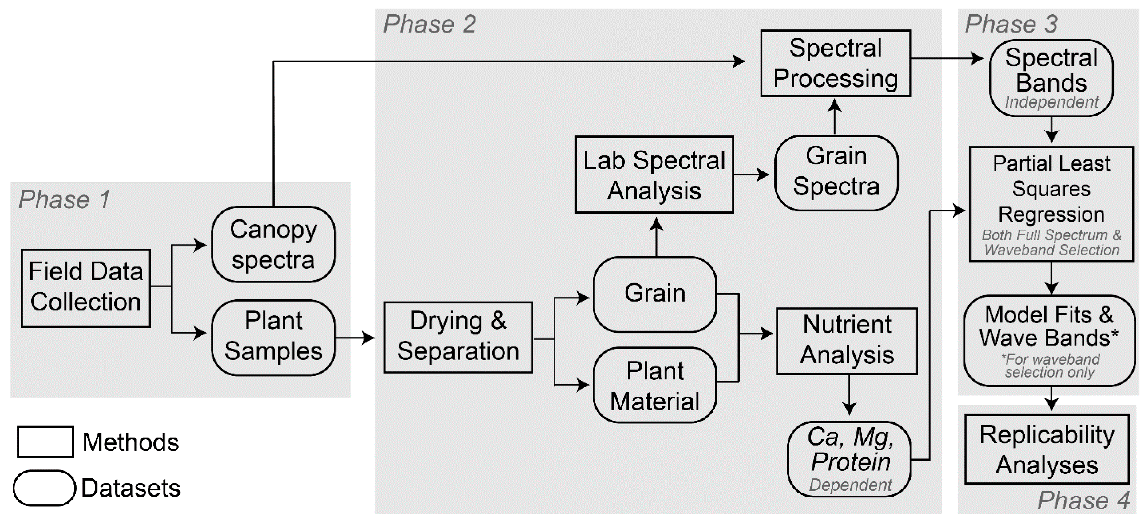
3. Analytical Methods

Partial least squares (PLS) regression was implemented to assess the relationship between reflectance (independent variable) and nutrient content (dependent variable) of both the plant and grain. PLS, which can also stand for projection to latent structures [43], was selected over other forms of regression because it accounts for overfitting errors common when analyzing hyperspectral data [13,44]. Briefly, PLS regression finds a set of components (called latent factors) from X, a matrix of predictors collected on the observations, that best predict Y, a matrix of dependent observations [43]. These latent factors, or latent vectors, are orthogonal, and thus explain as much of the covariance between X and Y as possible, often resulting in a smaller number of variables than principal component regression. PLS regression extracts X-scores from the latent variables to construct a model to predict the Y-scores. In PLS, the X- and Y-scores are subject to redundancy analysis that seeks directionality in factor space until the most accurate prediction is found [25,45]. When implementing PLS regression with hyperspectral data, it is important to ensure the number of latent variables does not far exceed the number of independent variables being used, as overfitting can occur [13].

3.1. Specification of the PLS Regression Model Using the Full Spectrum

The PLS equation follows a standard regression (Equation (1)):

$$\widehat{y}={\beta }_1{x}_1+{\beta }_2{x}_2+\cdots +{\beta }_k{x}_k+\epsilon$$

(1)

where the response variable $\widehat{y}$ is the nutrient value, and the predictor variables $x_1$ to $x_k$ are the reflectance (SG) or derivative (FD) values for bands 1 to $k$ (here, 277). ${\beta }_1$ to ${\beta }_k$ are the estimated weighted regression coefficients computed directly from the PLS loadings corresponding to the model with the optimal number of latent variables, and $\epsilon$ is the error vector. The optimal number of latent variables (NLV) is determined through a leave-one-out (LOO) cross-validation and assessed through the minimum root mean square error:

$$RMS{E}_{CV}=\sqrt{\frac{{{\displaystyle \sum }}_{i=1}^n{\left({\widehat{y}}_i^c-y_i^c\right)}^2}{n}}$$

(2)

where ${\widehat{y}}_i^c$ represents the predicted response when the model is built without sample i, $y_i^c$ represents the measured nutrient value for sample i, and n represents the number of samples used in the calibration [46]. Twelve, standard PLS regressions were performed, each corresponding to a dataset in Table 1, and each including the full set of 277 bands (PLS-Full).

3.2. PLS Regression with Waveband Selection

A modified form of PLS regression, known as the waveband selection (or iterative stepwise elimination) method, was developed to eliminate noisy and unhelpful predictors in hyperspectral studies [13,44]. Instead of including all 277 wavebands, the number is reduced iteratively [44] by dropping the least important wavebands (similar to stepwise linear regression). Waveband importance ($v_k$) is determined as:

$$v_k=\frac{\left|{\beta }_k\right|s_k}{{{\displaystyle \sum }}_{k=1}^K\left|{\beta }_k\right|s_k}$$

(3)

where ${\beta }_k$ and $s_k$ are the regression coefficient and standard deviation corresponding to waveband k. The selection begins with all 277 wavebands, and the waveband contributing least to the model (lowest $v_k$) is removed. The model (Equation (1)) is then re-run with 276 variables, and so on, until the maximum predictive capability is achieved [47]. 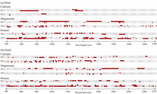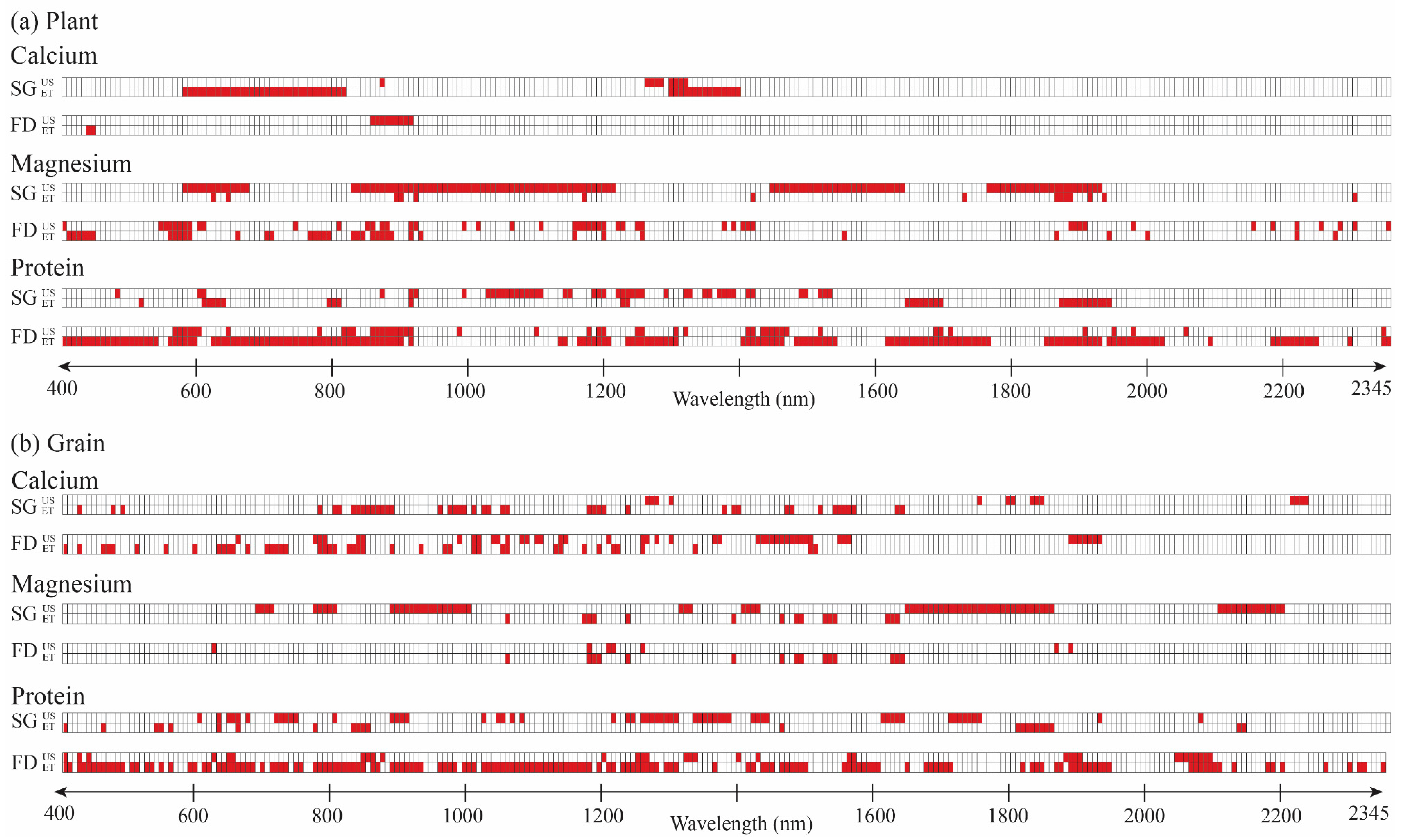A representation of the iterative processes to determine the maximum predictive capability is shown in Figure 5. This version of the model is hereafter referred to as PLS-Wave.

3.3. Predictive Ability of PLS Regression

To test the predictive capabilities of the PLS-Full and PLS-Wave models, we implemented a bootstrapping procedure by dividing the data into calibration (65–75%) and validation (25–35%) sets replacing the data of these sets $n=1000$ times (following [48,49]). After each separation, the models were calibrated (assessed through RMSE_CV) and then validated using root mean square error of prediction (RMSE_P):

$$RMS{E}_p=\sqrt{\frac{{{\displaystyle \sum }}_{i=1}^n{\left({\widehat{y}}_i^v-y_i^v\right)}^2}{n}}$$

(4)

where ${\widehat{y}}_i^v$ represents the predicted nutrient values, $y_i^v$ represents the measured nutrient values, and n represents the number of samples in the validation subset [46]. Mean coefficient of determination (R²), R² standard deviation (R² std.), and RMSE_P standard deviation (RMSE_P std) are also reported for the validation. PLS regressions were performed in Matlab v2016a (MathWorks, Sherborn, MA, USA).

3.4. Replication across Environments

To assess the replicability of the PLS-Full and PLS-Wave regression methodologies for predicting nutrient content across environments, we compared model performance between the US and ET using a difference of means (t-test) for each component–nutrient combination (e.g., grain–calcium, plant–calcium, etc.) between the two sites from the bootstrapped results. To compare the similarity of wavebands selected by the PLS-Wave model, the Jaccard index [50] was used to measure the overlap in selected wavebands compared to the total number of wavebands selected for each site (Equation (5)):

$$J\left(A,B\right)=\raisebox{1ex}{$|A\cap B|$}\!\left/ \!\raisebox{-1ex}{$|A\cup B|$}\right.$$

(5)

where A and B are the set of selected wavebands in the two locations, respectively. A Jaccard value of 1.0 indicates that the models for the two locations overlap completely in terms of the wavebands selected as important for prediction; 0 indicates the two locations share none of the same wavebands.

4. Results

4.1. Plant and Grain Nutrient Analyses

Plant nutrient values for Ca, Mg, and protein were considerably higher for the US compared to ET (

Table 2. Descriptive statistics for the calcium (Ca), magnesium (Mg), and protein measured for the plant and grain samples from each location.

	Nutrient	Descriptive Statistics
United States (US)		n	Min.	Mean	Max.	Range	SD
Plant	Ca (ppm mg/kg)	67	3760	6651	9360	5600	1371
	Mg (ppm mg/kg)	67	1860	2753	3620	1760	327
	Protein (%)	67	5.74	15.68	23.52	17.78	5.42
Grain	Ca (ppm mg/kg)	66	1620	2267	3240	1620	465
	Mg (ppm mg/kg)	66	1750	2015	2510	760	186
	Protein (%)	65	12.13	17.59	34.42	22.29	4.71
Ethiopia (ET)
Plant	Ca (ppm mg/kg)	78	437	1223	1772	1335	195
	Mg (ppm mg/kg)	79	115	740	1181	1066	297
	Protein (%)	79	3.02	5.77	9.93	6.91	1.69
Grain	Ca (ppm mg/kg)	78	716	1283	2128	1411	460
	Mg (ppm mg/kg)	79	270	553	841	571	155
	Protein (%)	79	8.16	10.84	14.57	6.41	1.43

). Mean Ca was five to six times higher; mean Mg almost four times higher; and mean protein nearly 2.5 times higher in the US. Results were similar for grain nutrients (Table 2), with values in the US typically two to four times higher than ET. Additionally, the standard deviation and ranges for Ca and protein at both the plant and grain level were higher in the US, except for Mg, which showed similar standard deviation and ranges across both locations for plant and grain.

4.2. Model Performance

4.2.1. Results for the PLS-Full Model

At the plant level (

Table 3. Partial least squares (PLS) regression and t-test results for the full spectrum model (PLS-Full) for plant and grain. SG: Savitsky–Golay; FD: First derivative; NLV: Number of latent variables; std: Standard deviation.

	Loc.	Calibration			Validation				Comparison
		NLV	R2CV	RMSECV	Mean R2	R2 Std	Mean RMSEP	RMSEP Std	t-test
Plant
Calcium
SG	US	2	0.53	935.79	0.52	0.12	976.86	168.52	−58.75 ***
	ET	3	0.10	229.07	0.18	0.14	221.14	42.02
FD	US	2	0.51	954.17	0.50	0.12	1000.47	156.54	−56.12 ***
	ET	1	0.09	231.48	0.20	0.17	233.25	82.71
Magnesium
SG	US	3	0.03	327.93	0.06	0.08	345.49	65.33	276.75 ***
	ET	7	0.87	108.63	0.86	0.04	117.70	16.45
FD	US	3	0.03	334.21	0.05	0.07	359.43	61.58	326.52 ***
	ET	7	0.88	104.66	0.86	0.04	117.47	16.25
Protein
SG	US	9	0.86	2.04	0.82	0.06	2.40	0.37	54.64 ***
	ET	5	0.18	1.34	0.38	0.12	1.42	0.16
FD	US	4	0.84	2.13	0.81	0.04	2.38	0.29	481.18 ***
	ET	2	0.41	1.30	0.44	0.12	1.35	0.15
Grain
Calcium
SG	US	7	0.88	159.89	0.87	0.04	176.55	28.41	−50.57 ***
	ET	14	0.78	216.06	0.74	0.07	253.12	31.16
FD	US	2	0.88	163.19	0.86	0.04	183.84	28.04	−44.96 ***
	ET	8	0.80	205.09	0.78	0.05	234.28	25.71
Magnesium
SG	US	6	0.71	99.49	0.70	0.10	108.77	18.81	219.53 ***
	ET	15	0.71	84.09	0.65	0.10	99.31	15.57
FD	US	3	0.73	96.49	0.72	0.10	104.89	17.96	144.8 ***
	ET	9	0.74	79.67	0.71	0.08	90.55	12.24
Protein
SG	US	15	0.93	1.23	0.90	0.05	1.59	0.51	−115.03 ***
	ET	5	0.47	1.03	0.49	0.14	1.09	0.18
FD	US	5	0.91	1.43	0.89	0.04	1.65	0.47	−106.51 ***
	ET	7	0.64	0.86	0.62	0.11	0.95	0.15

*** t-test significant at 0.001, ET served as first group.

, top), the PLS-Full models varied considerably in performance between the two sites with cross-validated calibration coefficients of determination (R²_CV) ranging from 0.03 (Mg US) to 0.88 (Mg ET) at the plant level. The validation coefficients of determinations (Mean R²) closely matched the calibration values, except in the case of ET (Ca and Protein (SG)) where the validation R² was approximately double that of the calibration. Interestingly, when comparing the US and ET, one generally outperformed the other, but the relationship changed depending on the nutrient. Differences in filtering (SG vs. FD) were largely negligible, with the exception of protein in ET, where the model fit for the FD was about twice that for the SG data (0.41 vs. 0.18). The bootstrapped R² values were normally or semi-normally distributed in all cases except for Mg in the US and Ca in ET (Figure S1, Supplementary Material). Importantly, t-test comparisons for replicability indicate the PLS-Full regression model did not replicate well across the two environments, with significant differences in fit for every nutrient at the plant level (Table 3, top).

At the grain level (Table 3, bottom), results were more consistent across the study sites and nutrients. This is believed to be the case in-part to grain spectral values measured in a controlled setting, while plants were measured in a field setting. Calibration R² ranged [0.47, 0.93], and validation R² ranged [0.49, 0.90] (Table 3). The results for ET protein using the SG data were a slight outlier though, and when considering only the FD values, the minimums increase to 0.64 and 0.62, respectively. The differences between the SG and FD filters were again negligible, except in the Mg ET case. The t-test comparisons for grain indicate the PLS-Full regression method did not replicate well across the environments.

4.2.2. Results for the PLS-Wave Model

At the plant level, the PLS-Wave models varied in performance in both environments with calibration R² ranging [0.11, 0.94] (

Table 4. Partial least squares (PLS) regression and t-test results for the waveband selection model (PLS-Wave) for plant and grain. SG: Savitsky–Golay; FD: First derivative; NLV: Number of latent variables; std: Standard deviation.

	Loc.	Calibration				Validation				Compare
		NLV	R2CV	RMSECV	# of Waves	Mean R2	R2 Std	Mean RMSEP	RMSEP Std	t-test
Plant
Calcium
SG	US	3	0.56	899.24	9	0.55	0.10	954.24	113.58	−52.36 ***
	ET	2	0.12	226.93	49	0.23	0.17	221.46	74.21
FD	US	1	0.53	929.65	9	0.55	0.10	937.88	125.67	−39.102 ***
	ET	1	0.11	228.37	2	0.25	0.19	219.72	75.70
Magnesium
SG	US	2	0.08	312.41	121	0.10	0.11	323.94	56.66	−11.34 ***
	ET	10	0.92	100.04	15	0.88	0.03	109.74	14.80
FD	US	4	0.30	277.97	50	0.28	0.14	296.41	48.51	−2.33 *
	ET	5	0.94	84.14	38	0.92	0.02	88.49	12.98
Protein
SG	US	6	0.88	1.84	46	0.88	0.04	1.93	0.29	−85.95 ***
	ET	3	0.45	1.25	31	0.46	0.11	1.32	0.12
FD	US	5	0.92	1.53	46	0.90	0.04	1.78	0.28	−72.48 ***
	ET	1	0.42	1.28	166	0.47	0.12	1.31	0.16
Grain
Calcium
SG	US	8	0.90	149.80	14	0.88	0.03	169.35	25.42	−40.05 ***
	ET	7	0.81	200.20	43	0.79	0.06	223.68	28.61
FD	US	2	0.91	142.23	47	0.89	0.04	156.88	25.36	17.45 ***
	ET	12	0.93	122.84	44	0.92	0.02	142.35	20.65
Magnesium
SG	US	4	0.73	96.74	77	0.73	0.10	102.28	22.78	−0.7781
	ET	12	0.73	80.54	15	0.73	0.07	87.75	11.56
FD	US	4	0.78	86.09	7	0.78	0.06	90.85	11.74	31.02 ***
	ET	8	0.87	56.29	33	0.85	0.04	63.38	9.02
Protein
SG	US	12	0.95	1.00	74	0.94	0.03	1.17	0.29	−94.58 ***
	ET	6	0.52	0.99	23	0.53	0.14	1.05	0.17
FD	US	4	0.93	1.24	33	0.92	0.03	1.43	0.33	−76.55 ***
	ET	7	0.67	0.82	159	0.65	0.11	0.91	0.14

* t-test significant at 0.05, ** at 0.01, *** at 0.001.

, top). Differences between the SG and FD were negligible in most cases. Fits for Mg in ET and Protein in the US were high (0.88–0.94), but there was little consistency across locations. t-test comparisons show significant differences in model performance for all nutrients/processing methods between the two locations indicating the PLS-Wave regression model did not replicate well in terms of predicting plant nutrients across these two environments.

At the grain level, the PLS-Wave models performed generally well for all nutrients across the two locations, with calibration R² ranging [0.52, 0.95] (Table 4, bottom). Fits for protein were lower for ET than US, but fits for Ca and Mg were similar. Bootstrapping resulted in normal and semi-normal distributions for all nutrients and processing (Figure S2, Supplementary Material). For Ca ET, a bimodal distribution was observed. Upon further investigation of the original Ca ET data, the distribution deviated from a normal distribution and instead was bimodal and skewed to the right, explaining the bimodal and skewed distribution of the R² bootstrapping values (Figure S2, Supplementary Material). t-test comparisons again indicate significant differences in all cases, despite similar R² values for some of the nutrient-component combinations, indicating the PLS-Wave regression model did not replicate well across these two environments.

In addition to significant differences in the model fits, the PLS waveband selection procedure also indicated considerable differences in the number and position of important wavebands for nutrient prediction (Figure 6). At both the plant and grain level, Jaccard indices were low (<0.2), with three instances having no overlapping bands (

Table 5. Jaccard index for similarity between bands selected by partial least square regression (PLS) for the US and Ethiopia (ET) datasets for the various models.

Plant	SG	FD
Ca	0.069	0.00
Mg	0.081	0.148
Protein	0.052	0.185
Grain	SG	FD
Ca	0.00	0.110
Mg	0.00	0.046
Protein	0.025	0.104

). For instance, nine wavebands were selected as important for predicting plant-level Ca in the US (SG): One at 760 nm, and eight from 1020–1060 nm (Figure 6). In contrast, the important bands for predicting Ca from the ET samples (SG) included fifteen bands positioned from 1045–1115 nm. The Jaccard index for this set was 0.069 (Table 5) indicating minimal overlap in the band positioning.

In summary, the results from this study indicate that the PLS regression, using both the full model and the waveband selection process, did not generate replicable findings across the two study areas. We found statistically significant differences in model fits for 11 of the 12 comparisons; only the model for grain Mg using the SG filtering (Table 4) was not statistically different. Even though model fits were not comparable, it is still possible for the wavebands identified as important for prediction to be similar. However, the Jaccard index (Table 5) and plots of the important wavebands for each model (Figure 6) indicate very little overlap in the important wavebands between the US and ET samples, further diminishing the case for replicability across these two study sites.

4.3. Combined Samples for Multiple Environments

Following the single environment analytics, we tested the performance of a PLSR for the two environments (US and ET) combined. We re-ran the analytics with the same methodologies for the PLS-Full and PLS-Wave models using the combined samples (named USET), and found this generally resulted in better model fits compared to the single sites for both calibration and validation for both the PLS-Full (

Table 6. Partial least squares regression (PLS) results for the full spectrum model (PLS-Full) for plant and grain using the combined United States and Ethiopia (USET) dataset. SG: Savitsky–Golay; FD: First derivative; NLV: Number of latent variables; std: Standard deviation.

	Calibration			Validation
	NLV	R2CV	RMSECV	Mean R2	R2 Std	Mean RMSEP	RMSEP Std
Plant
Calcium
SG	7	0.94	674.18	0.94	0.01	693.01	70.18
FD	5	0.94	684.48	0.94	0.01	694.93	87.95
Magnesium
SG	12	0.93	274.06	0.93	0.02	287.42	32.92
FD	6	0.93	269.72	0.93	0.02	289.64	37.94
Protein
SG	8	0.91	1.86	0.91	0.01	1.96	0.19
FD	4	0.90	1.94	0.90	0.02	2.03	0.22
Grain
Calcium
SG	14	0.90	216.52	0.80	0.03	240.30	22.71
FD	11	0.91	203.73	0.90	0.02	223.02	19.95
Magnesium
SG	14	0.97	118.87	0.97	0.01	128.61	13.50
FD	9	0.98	117.99	0.97	0.01	130.00	14.64
Protein
SG	15	0.93	1.25	0.92	0.02	1.37	0.25
FD	9	0.93	1.23	0.93	0.02	1.34	0.24

) and PLS-wave models (

Table 7. Partial least squares regression (PLS) results for the waveband selection model (PLS-Wave) for plant and grain using the combined Untied States and Ethiopia (USET) dataset. SG: Savitsky–Golay; FD: First derivative; NLV: Number of latent variables; std: Standard deviation.

	Calibration				Validation
	NLV	R2CV	RMSECV	# of Waves	Mean R2	R2 Std	Mean RMSEP	RMSEP Std
Plant
Calcium
SG	5	0.95	658.69	13	0.95	0.01	664.46	72.39
FD	4	0.95	664.55	38	0.94	0.01	690.87	79.27
Magnesium
SG	9	0.94	265.07	44	0.93	0.01	276.48	31.00
FD	5	0.94	261.27	112	0.94	0.01	271.65	33.62
Protein
SG	5	0.92	1.78	13	0.92	0.02	1.81	0.18
FD	8	0.93	1.68	52	0.92	0.02	1.79	0.16
Grain
Calcium
SG	11	0.91	206.43	59	0.90	0.02	221.41	21.83
FD	10	0.93	173.75	59	0.93	0.02	186.35	17.83
Magnesium
SG	12	0.98	106.71	39	0.98	0.00	114.98	11.90
FD	7	0.98	101.05	51	0.98	0.00	103.95	9.54
Protein
SG	10	0.94	1.12	19	0.94	0.02	1.16	0.19
FD	9	0.95	1.04	31	0.95	0.01	1.10	0.17

). Calibration and validation coefficients of determination (R²) were all greater than 0.9 for all plant and grain nutrients using both SG and FD data and for both the PLS-Full and PLS-Wave models. RMSE values from the validation were slightly higher than those from the calibration, which is expected, and RMSE_p values were all within 11 percent, so the models do not appear to be overfit.

5. Discussion

5.1. Replicability of Scientific Methods and Findings

Demonstrating that methods and findings can be replicated across studies is critical for the self-correcting mechanism of the scientific method to function properly and is imperative for generating solutions that can be applied widely. Hyperspectral data is commonly used in precision agriculture for predicting biochemical properties of vegetation and nutrients [18,26,51,52,53], yet the replicability of findings is rarely tested across different study sites. Scalable science is needed to develop solutions that can be applied globally. The adoption of PLS regression has provided a solution to some of the computational challenges when working with high dimensional, hyperspectral data in remote sensing in general and precision agriculture more specifically, but whether these solutions are transferable has not been widely explored. This study used hyperspectral data and in situ samples to build PLS models to predict plant and grain nutrients for tef and test the replicability of those models for predicting across different environments.

We found significant differences in model fits for both the PLS-Full and PLS-Wave models along with differences in the number and locations of wavebands deemed important for prediction with the PLS-Wave models. Differences in the optimal number and location of wavebands for predicting nutrients via plant canopy measurements may be influenced by varying management practices, such as differing irrigation practices, which may lead to variable water content in the crops [41]. The ET fields were rain fed while the US fields were irrigated through to harvest; therefore variable plant water content may have influenced which wavebands were selected, as water can cause access noise in spectral signatures. This noise is particularly prevalent in wavebands that are sensitive to O-H bonds, including the spectral range 971–1400 nm [54,55,56]. While we removed a portion of this range from our data (see Figure 4), it is possible remaining wavelengths were affected by noise making replication difficult.

The number of wavebands selected in the PLS models for ET was often less than the number selected for the US (Figure 5). This difference may reflect how the PLS models incorporate water-induced noise that may have been present in the US samples. These findings suggest that understanding how hyperspectral remote sensing methods, such as PLS regression, replicate across agricultural environments may require greater controls on the conditions under which crops are being cultivated. In addition to irrigation and other management differences, changes in latitude and sun angle could have led to differences in scattering and light absorption during field data collection [57], which would impact replication comparisons. However, hyperspectral readings for the grain samples were collected in a controlled laboratory setting with the same halogen lamp, so we can assume that any differences in wavebands were not the result of external factors (i.e., sun angles, latitudes, etc.).

When comparing the nutrient content of the grains, there were clear differences between the study areas (Table 2). These large differences likely result in varying chemical property relationships within the grain, which in turn can result in differential absorption and scattering of electromagnetic energy. The large variance amongst biochemicals within the grain may result in noise for some nutrients as nutrient reflectance properties are often associated with near or similar portions of the electromagnetic spectrum [41].

In short, had we completed this study only in the US, the PLS regression method (both with and without waveband selection) would have produced favorable findings for all three nutrients at the grain level, and for protein at the plant level. Similarly, had we completed this study only in ET, PLS regression would have also produced favorable findings for all three nutrients at the grain level, and for Mg at the plant level. Yet, even where favorable results were found in both environments (all three nutrients at the grain level), the model fits were statistically different, and the wavebands selected were not similar. This finding serves as a cautionary tale that urges researchers to refrain from placing too much confidence on R² values, which may not translate to different areas. Even when the R² values were superficially high, there were statistical differences in their values. This is not to suggest that hyperspectral investigations with PLS regression are not useful or valuable but rather that caution should be used when translating findings from one site to another.

5.2. Combining Samples from Multiple Regions

A valid question arises as to whether combining samples from multiple regions can make models more robust for prediction across environments. Higher performance was obtained when the US and ET samples were combined. However, these higher R² values are likely artifacts of a larger spread among the dataset (larger range of levels of nutrients across locations).

It is worth noting that in three instances, the RMSE_P from the combined USET dataset was greater than the minimum value of the nutrient in ET (see Table 2). These included Ca and Mg at the plant level for the PLS-Full model (Table 6) and Ca at the plant level for the PLS-Wave model (Table 7). Upon further investigation, it was determined that two of these samples were outliers (PLS-Full Mg and Ca), where the value was more than two standard deviations from the mean. Thus, these issues do not appear to be widespread or have a large impact on predictive capabilities of the models. However, it is important to keep this point in mind when combining data from differing regions with varying environmental factors and agricultural practices, where there may be large disparities in nutrient content. These disparities may result in the identification of between-site variation, requiring a greater variation of nutrient values to fully establish a generalized model.

Nevertheless, the results from the combined dataset are promising because they suggest that increasing within-sample variation can improve PLS model predictability across study areas. It is also worth mentioning that this practice could result in a reduction of accuracy of measurement, especially for field measurements, as the data may take on more noise. In this case, the use of single region analytics may be more beneficial. Nonetheless, improvement of predictability has been a similar finding in past studies that have referred to a need for global (i.e., USET) versus local (i.e., US and ET) modeling within similar measurement collections such as those in soil geochemistry studies [58,59]. Since it is unlikely though that this range of variation would be captured within a single site in many cases, it becomes necessary to combine samples from a variety of locations, and likely from a variety of study sites and research groups. To this point, we recommend building a more open and transparent culture of data sharing within the remote sensing community that can permit data sharing to advance our modeling capabilities and promote development of more generalizable predictive models. We recognize that a shift is already underway in many disciplines to promote data and code sharing, with some journals mandating these components accompany manuscript submission to allow reproducibility checks. Our findings here suggest that sharing data may have broader impacts beyond simply reproducing tests, but rather could result in more robust predictive models.

5.3. Non-Milled Grains

Since very few hyperspectral analyses have been performed on non-milled grains [26], we comment briefly on those aspects here. We generally found positive results using hyperspectral data with PLS regression to predict nutrient content of non-milled grains. While the reflectance measurements for these grain samples were collected in a controlled environment (i.e., a dark room using a contact probe), the coefficients of determination were noticeably higher for the grains compared to the plant canopy measurements collected in situ.

An interesting finding emerging from this research is that in the US, several blocks of wavebands corresponding to the VIS-NIR regions were identified as important for protein prediction when using FD values (Table S1, supplementary material). We compared these findings to other studies predicting protein from hyperspectral data [26,56,60]. We do see a considerable amount of overlap in the bands identified in this study for tef, and the bands identified in those studies for forage quality, cooked hams, and cereal grains (rice, oats, and maize), particularly for the FD transformation (

Table 8. Identification of matching bands associated with tef protein content that has also been identified as important protein indicators in past hyperspectral studies. Abbreviations: S: Savitsky–Golay; F: First derivative; B: Both; US: United States; ET: Ethiopia.

Object Measured	Band(s)	US Plant	ET Plant	US Grain	ET Grain	Paper
Forage	583		F		F	[60]
Forage	679		B	S	F
Forage	700–800 (Red Edge)	B	F	B	B
Forage	710			F	B
Cooked Hams	930				F	[56]
Cooked Hams	971	S	F	S	F
Cooked Hams	1051	F	F	S	F
Cooked Hams	1137		F	B
Cooked Hams	1165	F			F
Cooked Hams	1212	S	F
Cereal Grains	1216		F			[26]
Cereal Grains	1100–1400	B	F	B	B
Cooked Hams	1645		F		S	[56]
Cooked Hams	1682		S	F	F
Forage	2091		F			[60]
Forage	2128
Forage	2146			F	F

). However, as noted by Talens et al. [56], several of the band ranges found to be important across multiple studies for protein prediction do fall in the range impacted by O-H bonds. So, it is difficult to determine whether these consistencies are true positives or are being affected by other factors.

5.4. Potential Limitations

Environmental factors such as sun angle, soil types/moisture, agronomic practices, etc., can contribute to the reflectance and nutrient differences at the plant the level. Given the number of samples collected at each location, this study is not meant to be a representative sampling for all tef varieties at varying growth stages around the world. To establish more generalized models that can be applied to a broader range of locations/tef varieties, future studies should focus on obtaining a greater number of samples across a greater number of location for multiple tef varieties.

6. Conclusions

This study investigated the replicability of PLS regression methods, including PLS with waveband selection, for predicting nutrient content in plant and grain material across multiple environments. Using Eragrostis tef (tef) as a target crop, this study compared PLS model fits and selected wavebands across two environments in the U.S. and Ethiopia to determine the extent to which the methods and finding are replicable. Three main findings emerge from this study:

First, the model fits and wavebands selected as important for nutrient prediction were not replicable across the two study sites in the US and Ethiopia. Eleven of the 12 comparisons had statistically different model fits across 1000 bootstrapped iterations, and the Jaccard index for similarity indicated very low similarities in the wavebands selected.

Combining samples from both environments improved model fits, suggesting that increasing within-sample variation may improve the predictability of PLS models across study areas, though caution is reserved if great disparities in sample values are great. Our recommendation is to build a more open and transparent culture of data sharing within the remote sensing community that will permit data sharing in order to advance modeling capabilities and promote development of more generalizable predictive models.

Results using PLS regression with hyperspectral data from non-milled grains were generally positive, and wavebands for protein prediction generally agreed with other studies. While more research is needed to determine whether these consistencies are true positives or are affected by other factors, this study contributes to the gap in the literature related to non-milled grains.

References

1. Asendorph, J.B.; Conner, M.; De Fruyt, F.; De Houwer, J.; Denissen, J.J.; Fiedler, K.; Fiedler, S.; Funder, D.C.; Kliegl, R.; Nosek, B.A.; et al. Recommendations for increasing replicability in psychology. Eur. J. Pers. 2013, 27, 108–119. [Google Scholar] [CrossRef] [Green Version]
2. Camerer, C.F.; Dreber, A.; Forsell, E.; Ho, T.H.; Huber, J.; Johannesson, M.; Kirchler, M.; Almenberg, J.; Altmejd, A.; Chan, T.; et al. Evaluating replicability of laboratory experiments in economics. Science 2016, 351, 1433–1436. [Google Scholar] [CrossRef] [PubMed] [Green Version]
3. Begley, C.G.; Ioannidis, J.P. Reproducibility in science: Improving the standard for basic and preclinical research. Circ. Res. 2015, 116, 116–126. [Google Scholar] [CrossRef] [Green Version]
4. Ioannidis, J.P.; Stanley, T.D.; Doucouliagos, H. The power of bias in economics research. Econ. J. 2017, 127, F236–F265. [Google Scholar] [CrossRef]
5. Baker, M. Over half or psychology studies fail reproducibility test. Nat. News 2015. [Google Scholar] [CrossRef]
6. Baker, M. 1500 scientists lift the lid on reproducibility. Nature 2016, 533, 452–454. [Google Scholar] [CrossRef] [PubMed] [Green Version]
7. Bollem, K.; Cacioppo, J.T.; Kaplan, R.; Krosnick, J.; Olds, J.L. Social, Behavioral, and Economic Sciences Perspectives on Robust and Reliable Science; National Science Foundation: Arlington, VA, USA, 2015. Available online: https://www.nsf.gov/sbe/SBE_Spring_2015_AC_Meeting_Presentations/Bollen_Report_on_Replicability_SubcommitteeMay_2015.pdf (accessed on 6 April 2020).
8. National Academies of Sciences, Engineering, and Medicine (NAS). Reproducibility and Replicability in Science; National Academies Press: Washington, DC, USA, 2013. [Google Scholar]
9. Kedron, P.J.; Frazier, A.E.; Trgovac, A.B.; Nelson, T.; Fotheringham, A.S. Reproducibility and replicability in geographical analysis. Geogr. Anal. 2019. [Google Scholar] [CrossRef]
10. Anderson, K.; Milton, E.J. On the temporal stability of ground calibration targets: Implications for the reproducibility of remote sensing methodologies. Int. J. Remote Sens. 2006, 27, 3365–3374. [Google Scholar] [CrossRef]
11. Xu, C.; Holmgren, M.; Van Nes, E.H.; Hirota, M.; Chapin, F.S., III; Scheffer, M. A changing number of alternative states in the boreal biome: Reproducibility risks of replacing remote sensing products. PLoS ONE 2015, 10, e0143014. [Google Scholar] [CrossRef] [Green Version]
12. Ferreira, M.P.; Feret, J.; Grau, E.; Gastellu-Etchergorry, J.; Hummel do Amaral, C.; Shimabukuro, Y.; Filho, C. Retrieving structural and chemical properties of individual tree crowns in a highly diverse tropical forest with 3D radiative transfer modeling and imaging spectroscopy. Remote Sens. Environ. 2018, 211, 276–291. [Google Scholar] [CrossRef]
13. Kawamura, K.; Watanabe, N.; Sakanoue, S.; Inoue, Y. Estimating forage biomass and quality in a mixed sown pasture based on partial least squares regression with waveband selection. Jpn. Soc. Grassl. Sci. 2008, 54, 131–145. [Google Scholar] [CrossRef]
14. Nakaji, T.; Oguma, H.; Nakamura, M.; Kachina, P.; Asanok, L.; Marod, D.; Aiba, M.; Kurokawa, H.; Kosugi, Y.; Kassim, A.R.; et al. Estimation of six leaf traits of East Asian forest tree species by leaf spectroscopy and partial least square regression. Remote Sens. Environ. 2019, 233, 111381. [Google Scholar] [CrossRef]
15. Serbin, S.P.; Singh, A.; Desai, A.R.; Dubois, S.G.; Jablonski, A.D.; Kingdon, C.C.; Kruger, E.L.; Townsend, P.A. Remotely estimating photosynthetic capacity, and its response to temperature, in vegetation canopies using imaging spectroscopy. Remote Sens. Environ. 2015, 167, 78–87. [Google Scholar] [CrossRef]
16. Weiss, M.; Jacob, F.; Duveiller, G. Remote Sensing of agricultural applications: A meta-review. Remote Sens. Environ. 2020, 236, 111402. [Google Scholar] [CrossRef]
17. Schellberg, J.; Hill, M.J.; Gerhards, R.; Rothmund, M.; Braun, M. Precision agriculture on grassland: Applications, perspectives and constraints. Eur. J. Agron. 2008, 29, 59–71. [Google Scholar] [CrossRef]
18. Obermeier, W.A.; Lehnert, L.W.; Pohl, M.J.; Gianonni, S.M.; Silva, B.; Seibert, R.; Laser, H.; Moser, G.; Miller, C.; Luterbacher, J.; et al. Grassland ecosystem services in a changing environment: The potential of hyperspectral monitoring. Remote Sens. Environ. 2019, 232, 111273. [Google Scholar] [CrossRef]
19. Cho, M.A.; Skidmore, A.; Corsi, F.; Van Wieren, S.E.; Sobhan, I. Estimation of green grass/herb biomass for airborne hyperspectral imagery using spectral indices and partial least squares regression. Int. J. Appl. Earth Obs. 2007, 9, 414–424. [Google Scholar] [CrossRef]
20. Dechant, B.; Ryu, Y.; Kang, M. Making full use of hyperspectral data for gross primary productivity estimation with multivariate regression: Mechanistic insights from observations and process-based simulations. Remote Sens. Environ. 2019, 234, 111435. [Google Scholar] [CrossRef]
21. Fu, Y.; Yang, G.; Wang, J.; Song, X.; Feng, H. Winter wheat biomass estimation based on spectral indices, band depth analysis and partial least squares regression using hyperspectral measurements. Comput. Electron. Agric. 2014, 100, 51–59. [Google Scholar] [CrossRef]
22. Li, F.; Mistele, B.; Hu, Y.; Chen, X.; Schmidhalter, U. Reflectance estimation of canopy nitrogen content in winter wheat using optimized hyperspectral spectral indices and partial least squares regression. Eur. J. Agron. 2014, 52, 198–209. [Google Scholar] [CrossRef]
23. Meach-Hensold, K.; Montes, C.M.; Wu, J.; Guan, K.; Fu, P.; Ainsworth, E.A.; Pederson, T.; Moore, C.E.; Brown, K.L.; Raines, C.; et al. High-throughput field phenotyping using hyperspectral reflectance and partial least squares regression (PLSR) reveals genetic modifications to photosynthetic capacity. Remote Sens. Environ. 2019, 231, 111176. [Google Scholar] [CrossRef] [PubMed]
24. De Jong, S. SIMPLS: An alternative approach to partial least squares regression. Chemom. Intell. Lab. 1993, 18, 251–263. [Google Scholar] [CrossRef]
25. Geladi, P.; Kowalski, B. Partial least squares regression: A tutorial. Anal. Chim. Acta 1986, 185, 1–17. [Google Scholar] [CrossRef]
26. Caporaso, N.; Whitworth, M.B.; Fisk, I.D. Protein content prediction in single wheat kernels using hyperspectral imaging. Food Chem. 2018, 240, 32–42. [Google Scholar] [CrossRef]
27. Murphy, D.J. People, Plants, and Genes: The Story of Crops and Humanity; Oxford University Press: Oxford, UK, 2007; ISBN 9780199207145. [Google Scholar]
28. Vavilov, N. The Origin, Variation, Immunity and Breeding of Cultivated Plants; Chronica Botanica: Waltham, MA, USA; Stechert-Hafner: New York, NY, USA, 1951. [Google Scholar]
29. Flynn, K.C. Site suitability analysis for tef (Eragrostis tef) within the contiguous United States. Comput. Electron. Agric. 2019, 159, 119–128. [Google Scholar] [CrossRef]
30. Boe, A.; Somerfieldt, J.; Wynia, R.; Thiex, N. A preliminary evaluation of the forage potential of teff. Proc. S. Dak. Acad. Sci. 1986, 65, 75–82. [Google Scholar]
31. Bultosa, G.; Taylor, J.N.R. Encyclopedia of Grain Science; Wringley, C., Corke, H., Walker, C., Eds.; Academic Press: Oxford, UK, 2004; pp. 281–289. [Google Scholar]
32. Dekking, L.S.; Winkelaar, Y.K.; Koning, F. The Ethiopian cereal tef in celiac disease. N. Engl. J. Med. 2005, 353, 1748–1749. [Google Scholar] [CrossRef] [PubMed]
33. Gerbremariam, M.M.; Zarnkow, M.; Becker, T. Teff (Eragrostis tef) as a raw material for malting, brewing and manufacturing of gluten-free foods and beverages: A review. J. Food Sci. Tech. 2014, 51, 2881–2895. [Google Scholar] [CrossRef] [Green Version]
34. Hopman, G.D.; Dekking, E.H.A.; Blokland, M.L.J.; Wuisman, M.C.; Zuijderduin, W.M.K.F.; Schweizer, J.J. Tef in the diet of celiac patients in the Netherlands. Scand. J. Gastroenterol. 2008, 43, 277–282. [Google Scholar] [CrossRef]
35. Twidwell, E.K.; Boe, A.; Casper, D.P. Tef: A New Annual Forage Grass for South Dakota? South Dakota State University Extra Extension: Brookings, SD, USA, 2002; p. 8071. [Google Scholar]
36. Flynn, K.C.; Frazier, A.E.; Admas, S. Performance of chlorophyll prediction indices for Eragrostis tef at Sentinel-2 MSI and Landsat-8 OLI spectral resolutions. Precis. Agric. 2020, 1–15. [Google Scholar] [CrossRef]
37. National Forage Testing Association. Forage Analyses Procedures; South Dakota State University Extra Extension: Brookings, SD, USA, 1993; pp. 79–81. [Google Scholar]
38. Savitzky, A.; Golay, M.J.E. Smoothing and differentiation of data by simplified least squares procedures. Anal. Chem. 1964, 36, 1627–1639. [Google Scholar] [CrossRef]
39. Dawson, C.T.; Curran, P.J. A new technique for interpolating the reflectance red edger position. Int. J. Remote Sens. 1998, 19, 2133–2139. [Google Scholar] [CrossRef]
40. Frazier, A.E.; Wang, L.; Chen, J. Two new hyperspectral indices for comparing vegetation chlorophyll content. Geo Spat. Inf. Sci. 2014, 17, 17–25. [Google Scholar] [CrossRef]
41. Kokaly, R.F.; Asner, G.P.; Ollinger, S.V.; Martin, M.E.; Wessman, C.A. Characterizing canopy biochemistry from imaging spectroscopy and its application to ecosystem studies. Remote Sens. Environ. 2009, 113, 578–591. [Google Scholar] [CrossRef]
42. Soil Science Society of America (SSSA). Soil Testing and Plant Analysis, 3rd ed.; Soil Science Society of America: Madison, WI, USA, 1990; pp. 404–411. [Google Scholar]
43. Western States Laboratory Proficiency Testing Program. Soil and Plant Analytic Methods; Version 4.00; Western Regional Extension Publication: Pullman, WA, USA, 1997; pp. 117–119. [Google Scholar]
44. Abdi, H. Partial least squares regression and projection on latent structure regression (PLS regression). WIREs Comp. Stat. 2010, 2, 97–106. [Google Scholar] [CrossRef]
45. Kawamura, K.; Ikeura, H.; Phongchanmaixay, S.; Khanthavong, P. Canopy hyperspectral sensing of paddy fields at the booting stage and PLSL regression can assess grain yield. Remote Sens. 2018, 10, 1249. [Google Scholar] [CrossRef] [Green Version]
46. Wold, S.; Sjostrom, M.; Eriksson, L. PLS-regression: A basic tool of chemometrics. Chemom. Intell. Lab. 2001, 58, 109–130. [Google Scholar] [CrossRef]
47. Forina, M.; Lanteri, S.; Oliveros, M.C.C. Selection of useful predictors in multivariate calibration. Anal. Bioanal. Chem. 2004, 380, 397–418. [Google Scholar] [CrossRef]
48. Boggia, R.; Forina, M.; Fossa, P.; Mosti, L. Chemometric study and validation strategies in the structure-activity relationship of new cardiotonic agents. QSAR Comb. Sci. 1997, 16, 201–213. [Google Scholar] [CrossRef]
49. Efron, B. Bootstrap methods: Another look at the jackknife. Ann. Statist. 1979, 7, 1–26. [Google Scholar] [CrossRef]
50. Mutanga, O.; Skidmore, A.K.; Prins, H.H.T. Predicting in situ pasture quality in the Kruger National Park, South Africa, using continuum-removed absorption features. Remote Sens. Environ. 2004, 89, 393–408. [Google Scholar] [CrossRef]
51. Jaccard, P. Étude comparative de la distribution florale dans une portion des Alpes et des Jura. Bull. Soc. Vaud. Sci. Nat. 1901, 37, 547–579. [Google Scholar] [CrossRef]
52. Agelet, L.E.; Armstrong, P.R.; Clariana, I.R.; Hurburgh, C.R. Measurement of single soybean seed attributes by near-infrared technologies: A comparative study. J. Agric. Food Chem. 2012, 60, 8314–8322. [Google Scholar] [CrossRef] [PubMed]
53. Martinez-Valdivieso, D.; Font, R.; Gomez, P.; Blanco-Diaz, T.; Rio-Celestino, M.D. Determining the mineral composition in Cucurbita pepo fruit using near infrared reflectance spectroscopy. J. Sci. Food Agric. 2014, 94, 3171–3180. [Google Scholar] [CrossRef]
54. Phan-Thien, K.-Y.; Golic, M.; Wright, G.C.; Lee, N.A. Feasibility of estimating peanut essential mineral by near infrared reflectance spectroscopy. Sens. Instrum. Food Qual. Saf. 2011, 5, 43–49. [Google Scholar] [CrossRef]
55. Barlocco, N.; Vadell, A.; Ballesteros, F.; Galietta, G.; Cozzolino, D. Predicting intramuscular fat, moisture and Warner-Bratzler shear force in pork muscle using near infrared reflectance spectroscopy. Anim. Sci. 2006, 82, 111–116. [Google Scholar] [CrossRef]
56. Cozzolino, D.; Murray, I. Identification of animal meat muscles by visible and near infrared reflectance spectroscopy. LWT-Food Sci. Technol. 2004, 37, 447–452. [Google Scholar] [CrossRef]
57. Talens, P.; Mora, L.; Morsy, N.; Barbin, D.F.; ElMasry, G.; Sun, D. Prediction of water and protein contents and quality classification of Spanish cooked ham using NIR hyperspectral imaging. J. Food Eng. 2013, 117, 272–280. [Google Scholar] [CrossRef]
58. Jensen, J.R. Introductory Digital Image Processing: A Remote Sensing Perspective; Prentice Hall: Upper Saddle River, NJ, USA, 2016. [Google Scholar]
59. Wijewardane, N.K.; Ge, Y.; Wills, S.; Libohova, Z. Predicting physical and chemical properties of US soils with a mid-infrared reflectance spectral library. Soil Sci. Soc. Am. J. 2018, 82, 722–731. [Google Scholar] [CrossRef] [Green Version]
60. Guerrero, C.; Stenberg, B.; Wetterlind, J.; Viscarra Rossel, R.A.; Maestre, F.T.; Mouazen, A.M.; Zornoza, R.; Ruiz-Sinoga, J.D.; Kuang, B. Assessment of soil organic carbon at local scale with spiked NIR calibrations: Effects of selection nd extra-weighting on the spiking subset. Eur. J. Soil Sci. 2014, 65, 248–263. [Google Scholar] [CrossRef] [Green Version]
Figure 1. Locations of the four study sites.
Remotesensing 12 02867 g001
Figure 2. Methods flowchart detailing data collection and processing methods.
Remotesensing 12 02867 g002
Figure 3. Use of spectroadiometer in the field (left) and a close-up of Eragrostis tef (tef; right).
Remotesensing 12 02867 g003
Figure 4. Typical canopy spectra (noisy atmospheric windows removed) for tef (Eragrostis tef) showing (a) Savitsky–Golay filtered reflectance curve and (b) first derivative (FD) transformation.
Remotesensing 12 02867 g004
Figure 5. Representation of the iterative process to determine the number of wavebands via the waveband selection process. The number of wavebands is determined by the lowest RMSEcv value (dotted line), which in turn determines the coefficient of determination (solid line) using the given number of wavebands in the partial least square regression (PLS). Top figure is for the Savitsky–Golay filtered data. The bottom figure is for the first derivative.
Remotesensing 12 02867 g005
Figure 6. Selected wavebands (red) from the partial least square regression (PLS) using waveband selection for (a) plant, and (b) grain. Abbreviations: SG: Savitsky–Golay; FD: First derivative; US: United States; ET: Ethiopia.
Remotesensing 12 02867 g006