Article

Predicting Channel Conveyance and Characterizing Planform Using River Bathymetry via Satellite Image Compilation (RiBaSIC) Algorithm for DEM-Based Hydrodynamic Modeling

1
West Tennessee River Basin Authority, 3628 Eastend Dr, Humboldt, TN 38343, USA
2
Department of Civil and Environmental Engineering, Tennessee Technological University, 1020 Stadium Dr, Box 5015, Cookeville, TN 38505, USA
*
Author to whom correspondence should be addressed.
Remote Sens. 2020, 12(17), 2799; https://doi.org/10.3390/rs12172799
Submission received: 10 July 2020 / Revised: 20 August 2020 / Accepted: 24 August 2020 / Published: 28 August 2020
(This article belongs to the Section Remote Sensing in Geology, Geomorphology and Hydrology)

Abstract

:
Digital Elevation Models (DEMs) are widely used as a proxy for bathymetric data and several studies have attempted to improve DEM accuracy for hydrodynamic (HD) modeling. Most of these studies attempted to quantitatively improve estimates of channel conveyance (assuming a non-braided morphology) rather than accounting for the actual channel planform. Accurate representation of river conveyance and planform in a DEM is critical to HD modeling and can be achieved with a combination of remote sensing (e.g., satellite image) and field data, such as water surface elevation (WSE). Therefore, the objectives of this study are (i) to develop an algorithm for predicting channel conveyance and characterizing planform via satellite images and in situ WSE and (ii) to estimate discharge using the predicted conveyance via an HD model. The algorithm is named River Bathymetry via Satellite Image Compilation (RiBaSIC) and uses Landsat satellite imagery, Shuttle Radar Topography Mission (SRTM) DEM, Multi-Error-Removed Improved-Terrain (MERIT) DEM, and observed WSE. The algorithm is tested on four study areas along the Willamette River, Kushiyara River, Jamuna River, and Solimoes River. Channel slope and predicted hydraulic radius are subsequently estimated for approximating Manning’s roughness factor. Two-dimensional HD models using DEMs modified by the RiBaSIC algorithm and corresponding Manning’s roughness factors are employed for discharge estimation. The proposed algorithm can represent river planform and conveyance in single-channeled, meandering, wandering, and braided river reaches. Additionally, the HD models estimated discharge within 14–19% relative root mean squared error (RRMSE) in simulation of five years period.

Graphical Abstract

1. Introduction

Digital Elevation Models (DEMs) are commonly used for representing terrain in many geospatial, hydrologic, and hydraulic applications. Some of the commonly used DEM datasets have global coverage, including the Shuttle Radar Topography Mission (SRTM), Advanced Spaceborne Thermal Emission and Reflection Radiometer (ASTER), Advanced Land Observing Satellite Global Digital Surface Model (AW3D30), Multi-Error-Removed Improved-Terrain (MERIT), TerraSAR-X add-on for Digital Elevation Measurement (TanDEM-X), and Hydrological data and maps based on SHuttle Elevation Derivatives at multiple Scales (HydroSHEDS). These global DEMs are often the best available terrain data in many data-poor regions. Global DEMs are usually produced via remote sensing techniques and/or by merging multiple datasets. Thus, global DEMs are prone to errors in localized applications [1]. Studies have shown that fluvial features (e.g., river bathymetry, planform, and floodplain) are often not accurately represented in DEMs [2,3] and, thus, can introduce significant errors into hydrodynamic (HD) modeling. The errors may originate from the data source, data acquisition, signal processing algorithm, and/or spatial and temporal resolution of the DEM used in HD modeling [4,5,6,7,8,9].
Inaccurate representation of channel conveyance in a DEM can be averted by merging surveyed bathymetric data. However, a bathymetric survey can be both time and resource-intensive [10]. Therefore, DEM-based HD modeling in a data-poor region is often undertaken without modifying the DEM hence the changes in river bathymetry and planform are not accurately represented. Nevertheless, several studies have investigated on improving DEM accuracy over floodplains for hydrodynamic modeling [11,12]. For instance, MERIT DEM was introduced by minimizing elevation errors [13]. However, a unified DEM correction mechanism functional for both floodplain and channel is rare. It is particularly important in dynamic river systems where the river bathymetry, planform, floodplain connection, etc. are continuously evolving. This mutual interaction is eventually linked to the flow regime [14]. Therefore, it is important to search for a solution that can incorporate the three-dimensional configuration of a river into a DEM for an accurate representation of conveyance and planform into HD modeling. Such a solution would be especially useful for data-poor regions if it can perform well, despite limited field data. Certain gaps in field data can be addressed by remotely acquired data such as satellite imagery, which provides near real-time observation of a large part of the Earth and its waterbodies.
Satellite and aerial images have long been used to study river hydraulics [8,15]. Landsat-based river widths over long period have been correlated with altimetry-based water surface elevation (WSE) for producing equivalent cross-sections for an ungauged watershed [16]. However, this approach cannot predict riverbed elevation below the low water level and is limited to trapezoidal channel assumption. Their approach would be especially useful if depth prediction below the low water level could be made. A curve-fitting method is also developed to correlate remotely-sensed WSE and river width to predict river bathymetry [17]. However, this approach is only applicable to single-channeled rivers with predefined cross-sections. Several other methods based on open channel flow equations have been proposed to predict the depth of water (below low water level or a given stage) to improve remote sensing-derived DEMs [2,6,18,19]. These methods are commonly based on conceptual channel shapes (e.g., rectangular, prismatic, parabolic) for deriving equivalent cross-sections using known reach-averaged hydraulic properties (e.g., rating curve, channel slope, roughness factors, etc.). Two studies used conceptual cross-sections to calibrate channel dimension and Manning’s roughness factors simultaneously and found these two parameters can be interdependent [20,21]. Similarly, Manning’s roughness factor is found to be sensitive to DEM resolution for a DEM raster-based (i.e., DEM) steady HD model [22]. The dependency arises from the fact that a coarse DEM may show a higher river bed elevation due to the applied data interpolation method. Such simplification of river dimensions in large and morphologically complex rivers can lead to misrepresentation in spatial flood analysis. Additionally, DEMs only represent a snapshot in time, therefore, it becomes outdated if the river planform is changed. Nevertheless, remote sensing data such as time series of satellite imagery has the capability of capturing spatial and temporal dynamics of large and complex rivers.
A few remote sensing-based methods have been developed to characterize river dimensions [23,24,25,26,27]. Some of these methods utilize passive optical imaging to map river depths. The fundamental principle in retrieving river depth from a passive optical image is that depth in shallow clear-flowing water is linearly (or monotonically) correlated to an image-derived quantity, which is a function of reflectance [28]. These methods have shown promising results in clear-flowing water, but their performance over turbid water and unsurveyed reaches are limited. Two methods named Hydraulically Assisted Bathymetry (HAB), and Flow Resistance Equation-Based Imaging of River Depths (FREEBIRD) are capable of mapping bathymetry in the absence of field-based depth measurements [24,29]. However, they require an initial estimate of the channel aspect (width-to-depth) ratio or knowledge of discharge [30]. Another method using Image-to-Depth Quantile Transformation (IDQT) was proposed for inferring river bathymetry using images [30]. This technique can be applied in the absence of depth data for depth-to-image quantity calibration and does not necessarily require a linear correlation. IDQT can replace field surveyed depth measurements with a probabilistic distribution of the ratio between spot depths and reach-averaged depth. However, obtaining reach-averaged depth might be challenging in a river where no prior knowledge of the river bathymetry is available. Another method was presented based on entropy theory in which Moderate Resolution Imaging Spectroradiometer (MODIS) data and a predefined horizontal velocity distribution along the channel cross-section were used to predict bathymetry [31]. This study noted the method’s applicability in narrow rivers is uncertain due to the spatial resolution of MODIS data (250 m). Additionally, the elliptical velocity distribution approximation might not be valid for braided or meandering river sections where maximum velocity is dictated by river morphology. Therefore, this approach is only applicable to selected river sections.
To summarize, existing indirect depth measurement techniques are either dependent upon prior knowledge and/or predefined cross-section shapes. A study based on an assessment of different bathymetry prediction methods noted that the predefined river cross-section assumption might be acceptable for one-dimensional (1D) modeling but its usefulness for two-dimensional (2D) models is uncertain [32]. This study also recommended that a more robust and spatially accurate bathymetry prediction method is needed for large rivers and streams. The existing bathymetry prediction methods usually approximate river cross-sections at defined transects and interpolate in between those transects. This is a critical obstacle to spatial flood analysis via 2D modeling because river width and planform is not the same along the river length. Additionally, reliance on the dimension, discharge, and/or velocity data make them inapplicable in data-scarce areas. Therefore, being able to utilize minimal hydrologic data for prediction of river bathymetry and hence conveyance could be beneficial. Linking WSE with earth-observing satellite images can be particularly useful because ground-based WSE measurements are more frequently available than flow measurements and current satellite imaging missions scan a large part of the earth at a convenient time interval (e.g., approximately 16 days for Landsat). Additionally, space-based WSE measurement is already being performed from current missions such as Jason-3, Satellite with ARgos and ALtiKa (SARAL), and Ice, Cloud and land Elevation Satellite-2 (ICWSat-2) [33]. Future missions, such as National Aeronautics and Space Administration’s (NASA) Surface Water and Ocean Topography (SWOT) are also scheduled to estimate WSE, water mask (water extent), and slope [34] of rivers wider than 100 m. Thus, a WSE and satellite image-based conveyance-prediction algorithm can potentially be used in remote, inaccessible, and truly data-poor regions in the future. Hence, the objectives of this study are:
  • to develop an algorithm for predicting channel conveyance and characterizing planform via satellite images and observed (in situ) WSE as input;
  • to estimate river discharge using the predicted conveyance via an HD model after applying the algorithm.
In the following sections, a novel algorithm named the River Bathymetry via Satellite Image Compilation (RiBaSIC) is proposed and validated. The purpose of this research is conveyance prediction and planform characterization of a river reach using publicly available remote sensing data and observed WSE that would be suitable for 2D HD modeling. In this paper, the terms “observed” refers to any data that is measured in the field or surveyed or processed using measured data (e.g., streamflow, rating curve).

2. Materials and Method

The methodology of this research follows a two-step approach that includes: (i) developing a river conveyance prediction and planform characterization algorithm via satellite images and observed WSE (ii) estimating river discharge using a moderate resolution (i.e., 30 m) global DEM-based HD model after applying the conveyance-prediction algorithm. The input data needed for this study are satellite images, observed WSE, and DEM. A brief description of the methodology is provided in the following subsections.

2.1. Developing a River Conveyance Prediction and Planform Characterization Algorithm via Satellite Image and Observed WSE

Satellite images are useful in analyzing the change of river extent over time. An algorithm to predict river conveyance via linking satellite images and observed WSE is presented in the following paragraphs. A schematic of the method is shown in Figure 1, a qualitative example is provided in Appendix A, and a list of acronyms is presented in Abbreviations. The only observed data needed for proposed RiBaSIC algorithm is time series of WSE at one location near the study area; thus, it can be applied to a region where hydrologic (i.e., flow, rating curve) and hydraulic data (e.g., roughness factors, channel aspect, conceptual channel shape, etc.) are limited. However, the length of the study area should be limited such that it does not include any major inflow or outflow and seasonal WSE variation is uniform within the reach length. To execute the algorithm, a programming language (MATLAB) and a geospatial analysis tool (ArcGIS) is used. The study area for implementing the RiBaSIC algorithm is hereafter called “RiBaSIC extent”. The assumptions for executing the RiBaSIC algorithm is also listed below:
  • the WSE of the study area is not affected by the tide;
  • the seasonal variation of WSE within the study area is uniform;
  • the river reach maintains flow continuity meaning no major lateral inflow or outflow;
  • the reach for which the channel profile is determined does not have any abrupt changes in elevation such as a cascade or rapid;
  • the river reach is free from any natural and/or artificial storage areas such as lakes;
  • no significant natural and/or artificial changes happened in the river planform or conveyance within the study period;
  • the width of the actively flowing channel increases with increasing WSE;
  • the satellite image has sufficient bands to cover the visible and Infra-Red (IR) spectrum;
  • the river bankfull width is at least three times the spatial resolution of the satellite image for identifying the channel and side slopes;
  • there are a sufficient number of satellite images available to capture a minimum of one hydrologic cycle.

2.1.1. Time Window Selection

The first task of the RiBaSIC algorithm is to select a time window within which planform shifting (i.e., change in riverbank lines, islands, confluence, etc.) in the RiBaSIC extent is nominal. This can be done by comparing satellite images of the RiBaSIC extent immediately before and after the selected study period. Additionally, the time window should not include any major natural (such as avulsion, cutoff, meander migration) or manmade (such as dredging, channelization) alteration of the river conveyance. However, it is recommended that the time window should not be less than one year so that the seasonal variation of the river stage is captured.

2.1.2. Input Data Processing

The second task for the algorithm is processing the input data for implementing in RiBaSIC algorithm. Available satellite images within the time window for the RiBaSIC extent is collected. For ease of processing, it is recommended that all the collected images have the same source and same spatial resolution. Historic WSE for a nearby streamflow gauge is also collected from which the lowest water level (LWL) is calculated. It should be noted that low water level is the minimum WSE for any given period (e.g., one hydrologic year) but LWL is the minimum WSE from the entire record of historic WSE.
An approximate river polygon (covering the main channel, overbank areas, and adjacent floodplains) for RiBaSIC extent is delineated and converted to a raster with the same spatial resolution and cell alignment as the satellite image. The raster is then converted to an Environmental Systems Research Institute (ESRI) point shapefile (hereafter called as “river points”) where each point represents the center of a corresponding raster cell and has a unique identification number (hereafter called as “cell id”).
A DEM for the RiBaSIC extent is also collected. This is used to determine a longitudinal channel profile of the river. The profile is estimated by fitting DEM elevations and distance along the center of the main channel of the river. The second-order polynomial channel profile is used because a river profile may not be linear in longer (for example in watershed-scale) reach lengths [35]. The elevation (z) at a distance x is expressed as Equation (1) by this channel profile. The coefficients a, b, and c are derived by fitting DEM elevations and distance along the main channel of the river. Differentiation of the channel profile provides Equation (2) that represents the tangential or linear slope of the channel profile at distance x.
Channel   profile   Z = a x 2 + b x + c
Linear   slope :   S = d z d x = 2 a x + b
where, x = distance.

2.1.3. Shoreline Delineation

The third task is to determine the edges of the water extent at different WSE following an approach similar to the waterline method [12,36,37,38,39,40]. To determine the edges of the water, all the images within the time window are processed using the Equation (3) to calculate a Normalized Difference Water Index (NDWI) [41]. During this process, cloudy pixels in an image are filtered out via a cloud-masking tool called “Fmask” [42,43]. A positive NDWI indicates water whereas a zero or negative value indicates a non-water surface. However, to avoid noisy pixels (e.g., saturated soil), small NDWI values (NDWI < 10) are excluded and, hence, the threshold is set as 10.
NDWI = 100 Green   band NIR   band Green   band + NIR   band
where, NIR = Near Infra-Red.
The wet pixels identified in each image are assigned WSE corresponding to the image acquisition date. After compiling NDWI for all the images, the lowest WSE for each cell is calculated. The lowest WSE per cell estimated from NDWI is, hereafter, called “shoreline elevation” for respective river points (or cells).

2.1.4. Bathymetry Prediction

The fourth task of the RiBaSIC algorithm is bathymetry prediction. It has multiple steps that are presented below.
  • Image Processing: typically, water reflects 10% of the incoming radiation that is limited to visible to NIR spectrum but soil reflects throughout the IR bands [44,45]. The highest reflectance is provided by turbid water [45] which is commonly found in river channels. Additionally, pixels in a river channel are mainly covered by soil that is periodically inundated. Therefore, short wavelength infra-red (SWIR) bands are useful for separating inundated and non-inundated river pixels in an image. So, the ratio of visible and IR (NIR and SWIR) bands are used in this step for predicting bathymetry. Similar to Section 2.1.3, cloud-covered pixels are removed first via the “Fmask” tool. Once the cloudy pixels are removed, Equation (4) is used to calculate a novel index called Average Difference Water Index (ADWI) for each cell. The ADWI values are stored as integers where a positive index value indicates a channel cell (inundated) and a negative indicates non-channel (non-inundated) cell. The selected channel cells in each image are assigned WSE of the image acquisition date.
    Average   Difference   Water   Index   ( ADWI )                           = 100 avg     of     visible     bands avg     of     IR     bands avg     of     visible     bands + avg     of     IR     bands
  • Generating Library of ADWI and WSE: a library of ADWI and corresponding WSE for each cell within the RiBaSIC extent (also referred to as river points) is generated. The library is used to determine the lowest and highest WSE at which a cell is found to be within a channel (LWSE and HWSE, respectively) along with the highest WSE at which a cell is found to be dry or non-channel (DWSE). If any cell is found to be in the channel at only one instance, then that WSE would be categorized as LWSE for that cell. The ADWI value corresponding to a cell’s LWSE is stored as that cell’s “Low Water Index” (LWI).
  • ADWI versus Depth Correlation: the historic LWL of the nearby streamflow gauge is required to establish the ADWI versus depth correlation. If the riverbed is static (i.e., no significant bed level aggradation-degradation), then the thalweg elevation (lowest elevation of the riverbed) should be less than the LWL. Riverbed elevation for each cell or river point is approximated by two trials using the equations provided below.

1st Trial

In the 1st trial, thalweg elevation is assumed the same as LWL.
Hence, thalweg elevation, Zt = LWL.
Where, LWL = lowest water level from historic data
Depth     factor ,   f = maximum   WSE   in   image   acquisition   dates Z t ( maximum - minimum ) WSE   in   image   acqusition   dates
Then, for any cell that is wet more than once,
Factored     depth ,     d f = f ( HWSE LWSE )
where
HWSE   =   Highest     WSE     at     which     the     cell     is     found     in     channel
LWSE   =   Lowest     WSE     at     which     the     cell     is     found     in     channel
Approximate     bed     elevation ,     Z = maximum     of     [ DWSE     and     ( HWSE d f ) ]
where
DWSE   =   Highest     WSE     at     which     the     cell     is     found     dry
For each image, depth values per cell are calculated by subtracting approximate bed elevation (Z*) from the corresponding WSE.
Depth     during     satellite     image     scene     i ,   d i = WSE i Z
ADWI     corresponding     to     d i = ADWI i
After analyzing each cell in all the images, ADWIs are sorted and corresponding depths are stored. For each integer ADWI value, the average depth (from all the cells in every image that has the same ADWI) is calculated to create an ADWI versus depth correlation.

2nd Trial

Ideally, the thalweg elevation of a river should be lower than LWL. Therefore, the depth values obtained in the 1st trial is used to make an approximation for the depth of thalweg at LWL. This depth value is called delta (Δd) which is approximated as the first one percentile of all the average depth values calculated in the 1st trial. Thus, thalweg elevation in the second trial is estimated as the following:
Z t = LWL Δ d
After updating the thalweg elevation (Zt), the same approach as the 1st trial is repeated. By the end of the 2nd trial, the final ADWI versus depth correlation is established. This correlation is used as a lookup table for estimating ADWI bathymetry.
ADWI bathymetry: the ADWI versus average depth correlation is used to derive the river bathymetry. For each cell, the average depth corresponding to LWI (from ADWI versus average depth correlation) is subtracted from LWSE to get the bed elevation. This is hereafter called “ADWI bathymetry”.

2.1.5. Post-Processing

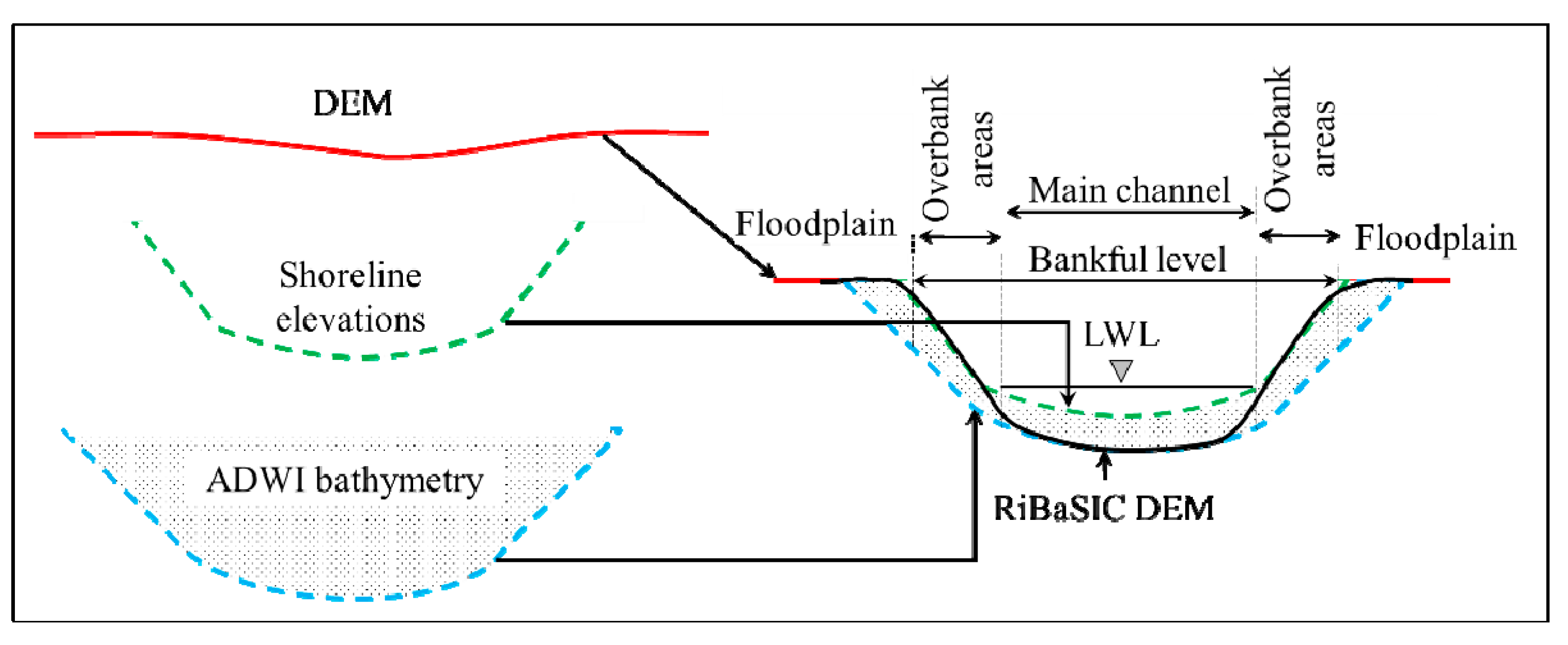
The last task of the RiBaSIC algorithm is post-processing the shoreline and bathymetry elevations for the cells obtained in Section 2.1.3 and Section 2.1.4. Post-processing is needed for accurately assigning bathymetric, overbank and floodplain elevations of the river reach. It has three main steps that are presented below with a schematic in Figure 2.
  • Slope Transferred Elevation: the shoreline elevations and ADWI bathymetry elevations for the cells obtained in Section 2.1.3 and Section 2.1.4 are transferred to their geographic locations using the channel profile [refer to Equation (1)] and distance.
  • RiBaSIC Bathymetry: the shoreline delineation method using NDWI (please refer to Section 2.1.3) cannot predict the bathymetry in the main channel that is under water during the dry season. Therefore, the shorelines delineated from a dry season cloud-free image is assumed as the main channel. The cells inside the main channel are assigned ADWI bathymetry estimated in Section 2.1.4. The cells outside of the main channel but found wet in at least one image in Section 2.1.3 are considered as overbank areas. The shoreline elevations are assigned for cells in overbank areas. This merged dataset is, hereafter, called “RiBaSIC bathymetry”.
  • RiBaSIC DEM: the cells that are neither in the main channel nor in overbank areas are considered as floodplain areas. The elevations of the floodplain cells are obtained from a DEM. Finally, RiBaSIC bathymetry and the DEM are merged to create a raster surface that is, hereafter, called “RiBaSIC DEM”.

2.2. Discharge Estimation from HD Model Using a Moderate Quality Global DEM

Discharge estimation using observed WSE and moderate resolution DEM is performed via Hydrologic Engineering Center’s River Analysis System (HEC-RAS) model version 5.0.6 that allows 2D HD simulation. The study area for HD modeling is hereafter called a “model extent”. Observed WSE is used as the upstream boundary condition, Manning’s n values are used to define surface roughness and friction slope at normal depth is used as the downstream boundary condition. The friction slope at downstream is determined by differentiating the second-order channel profile [please refer to Equation (2) in Section 2.1.2] at the downstream location. The methodology for approximating Manning’s roughness factors is presented in the next sub-section.

2.2.1. Manning’s Roughness Factor Approximation

To perform HD modeling in this study, appropriate Manning’s n factors are needed. Since the RiBaSIC algorithm is intended to be applied in regions without prior knowledge of geomorphology and flow, the authors demonstrate an approach to approximate Manning’s roughness factors using RiBaSIC bathymetry and channel profile. Based on a review of the literature, several equations are available for predicting Manning’s roughness factors from the morphological properties of rivers. A few equations are selected that predict Manning’s roughness factors from hydraulic radius and slope (refer to Table 1). These equations are chosen because slope can be obtained from channel profile [assuming channel slope (S) ≈ water surface slope (Sw) ≈ energy gradient (Sf)] and hydraulic radius can be obtained from RiBaSIC bathymetry. Each of these equations is developed for particular types of rivers and they may not be the same as the given study areas. Hence, a Manning’s roughness factor approximation methodology is followed for the model extents of this study. It has five steps that are presented below with a schematic in Figure 3.
Step 1:
hydraulic radius of the cross-sections at upstream of the model extent is calculated.
Step 2:
linear slope at the upstream location is estimated. For more details on estimating linear slopes at upstream and downstream locations, the readers are referred to Section 2.1.2 and Appendix A.
Step 3:
Manning’s n values for the upstream location is calculated using the equations listed in Table 1.
Step 4:
any Manning’s n value less than 0.010 is considered as “unreasonable” for natural rivers (for the flow within the main channel) and hence discarded. This filtering is important because Manning’s n values can be as small as 0.025 for minor streams (width at flood stage < 30 m) although for major streams, the value can be smaller than that of a minor stream of similar characteristics [51]. Moreover, alluvial sand bed rivers could have Manning’s n value ranging from 0.018 to 0.035 [52]. The smallest prescribed Manning’s n value is 0.016, which is applicable for straight and uniform earthen channels [51]. Therefore, Manning’s n value as small as 0.010 is likely to be an erroneous one and needs to be excluded.
Step 5:
the average of Manning’s n estimates (from step 4) is calculated.
The Manning’s roughness factor downstream of the model extent is also estimated following the above-mentioned steps. The upstream and downstream Manning’s roughness factors are spatially interpolated along the river length to use in HD modeling.

2.2.2. Study Areas

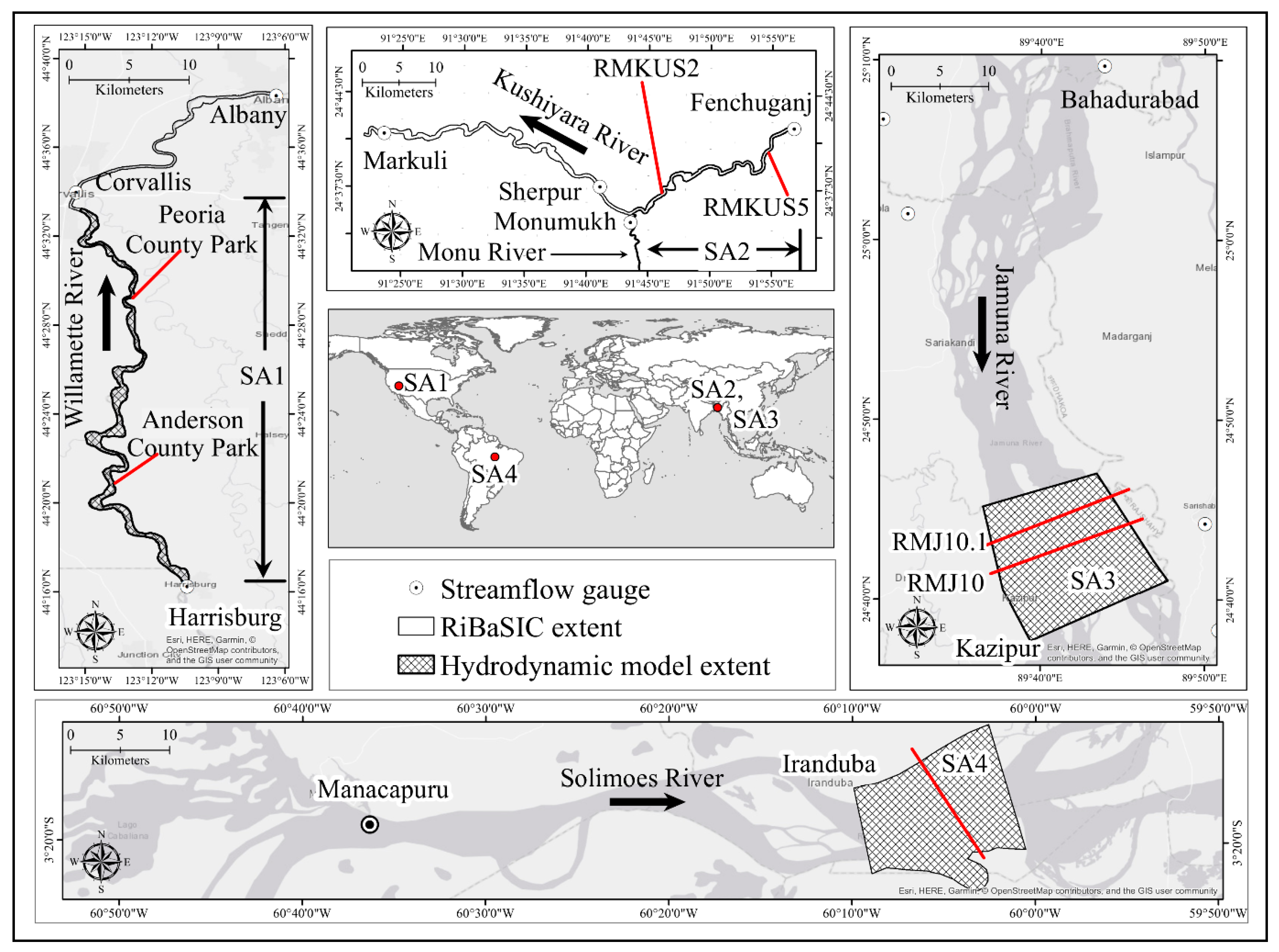
Four study areas are selected where the RiBaSIC algorithm is tested and 2D HD modeling is performed. The four study areas are Willamette River in Oregon, USA (SA1), Kushiyara River in Bangladesh (SA2), Jamuna River in Bangladesh (SA3), and Solimoes River (SA4) in Brazil. The study areas are chosen to cover a wide range of rivers spread across different geographic locations. The RiBaSIC extent and model extents are the same for SA3 and SA4 but the model extents in SA1 and SA2 are shorter than their RiBaSIC extents to save the computational time of HD simulation. The HD model for each study area is simulated for five consecutive years to determine the efficiency of the proposed methodology for estimating long-term flow patterns. The study areas are shown in Figure 4 and a brief description is presented in Table 2.

2.2.3. Data

Satellite imagery, WSE, and DEM are the main data needed for executing the RiBaSIC algorithm. Landsat satellite image is collected from the United States Geologic Survey (USGS) EarthExplorer database. Observed WSE is collected from USGS, Bangladesh Water Development Board (BWDB), and the SO-HYBAM (previously known as Environmental Research Observatory). The one-arc second (~30 m) SRTM DEM is also collected from USGS EarthExplorer for obtaining channel profile. Additionally, MERIT DEM is collected from the Institute of Industrial Sciences at The University of Tokyo. MERIT DEM is used for representing floodplain elevation because it is derived from SRTM version 2.1 and AW3DDEM (ALOS: Advanced Land Observing Satellite, World 3D-DEM) that has an improved representation of floodplains compared to SRTM [13]. Since the RiBaSIC bathymetry has a spatial resolution of one-arc-second, MERIT DEM is resampled to one-arc second from three-arc second (~90 m) using bilinear interpolation for producing RiBaSIC DEM. Surveyed bathymetry data and observed discharge are also collected from nearby streamflow gauges for validating RiBaSIC algorithm and accuracy assessment of estimated discharge. The available literature is also studied to fill up the gaps in field data.

3. Results

The RiBaSIC algorithm is developed (see Section 2.1) and applied to produce RiBaSIC DEM for the study areas. The validation of the algorithm and performance of HD simulations using The RiBaSIC DEM are presented in this section.

3.1. Validation of the RiBaSIC Algorithm

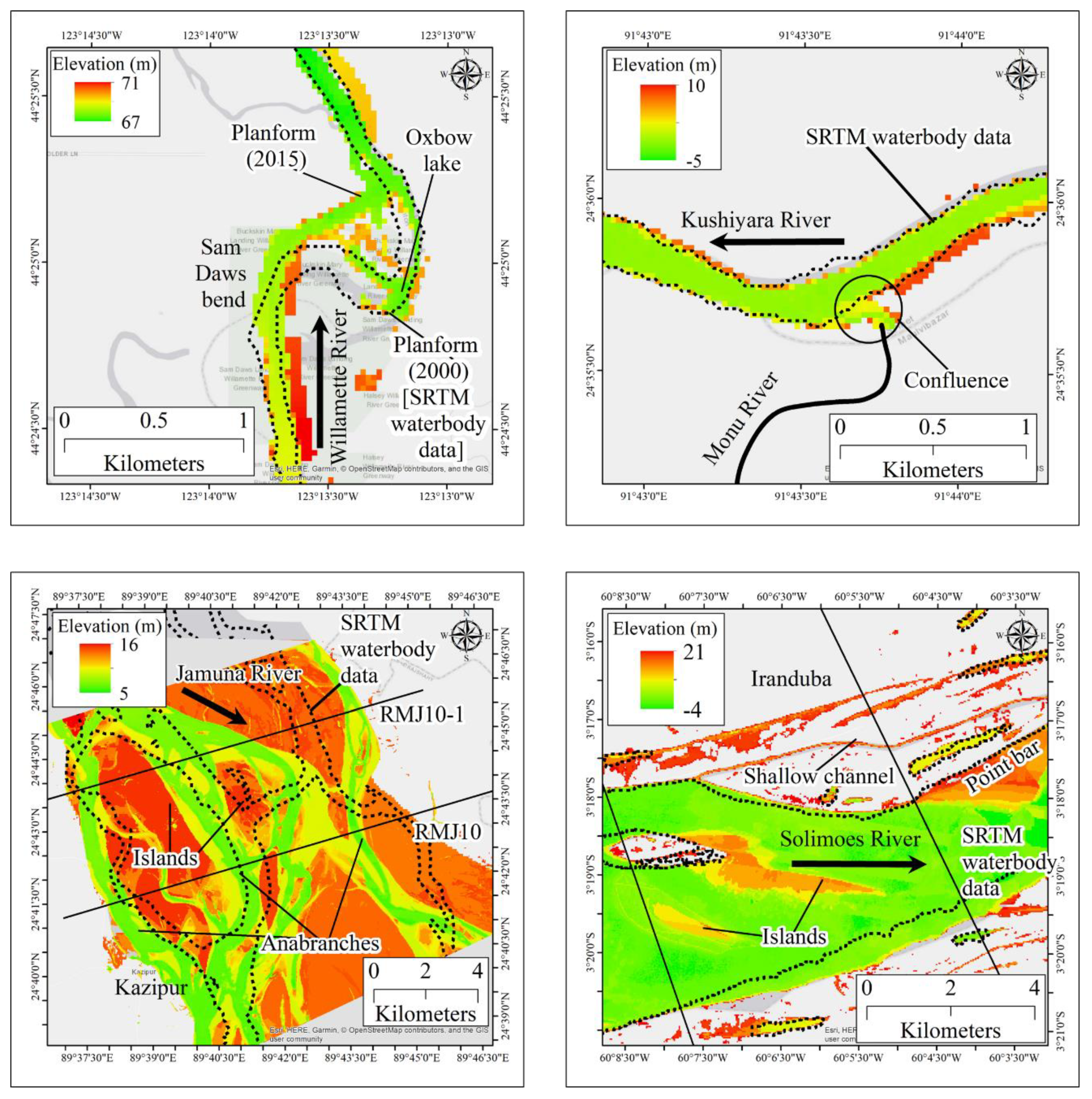
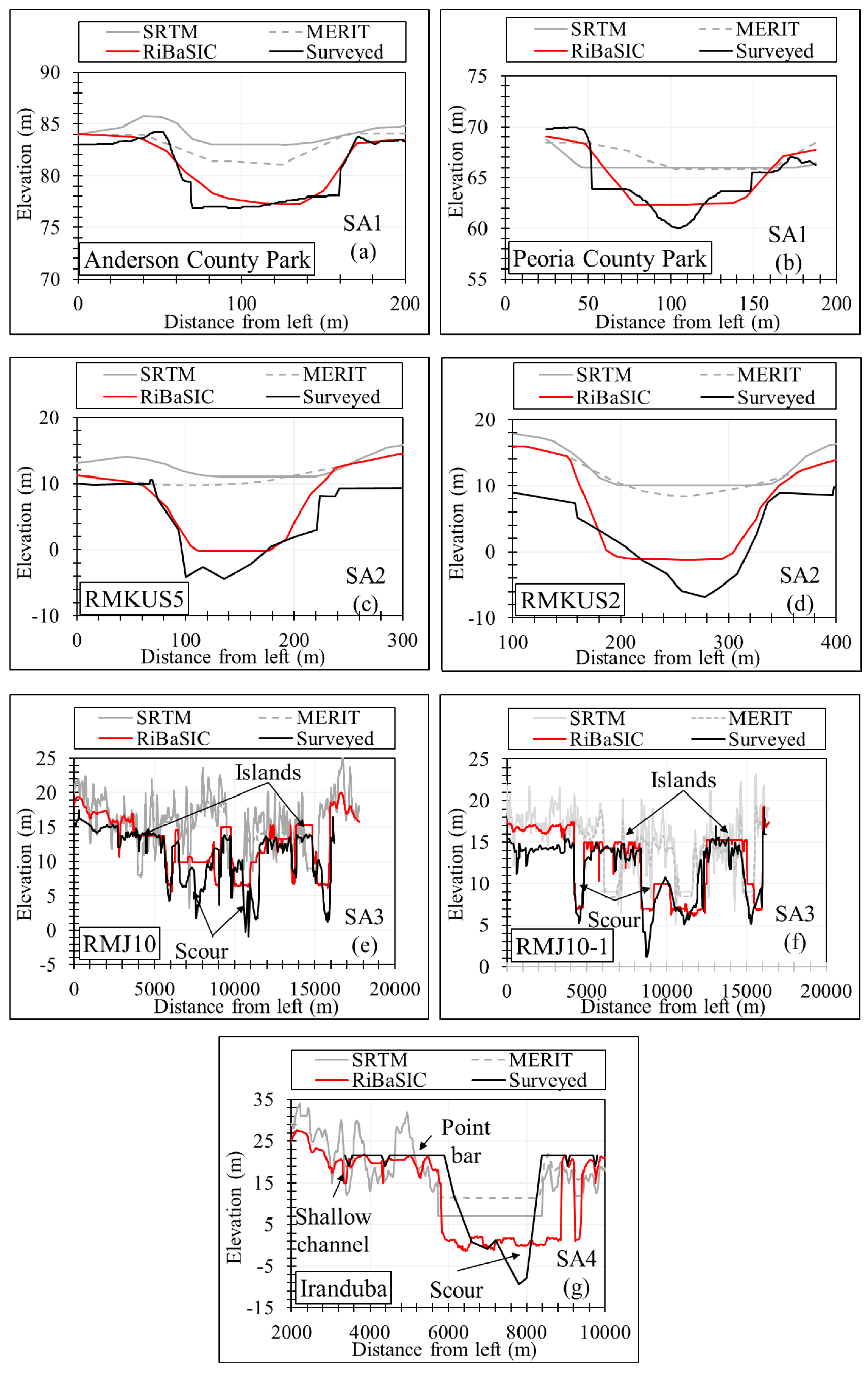
RiBaSIC algorithm is implemented in the study areas following the methodology presented in Section 2.1 and data listed in Table 2. The spatial resolution of the RiBaSIC bathymetry raster is the same as the Landsat image (30 m). Therefore, the spatial resolution of RiBaSIC DEM (RiBaSIC bathymetry merged with resampled MERIT DEM) is also one arc-second or 30 m. A planform view of the RiBaSIC bathymetries over some reaches in the study areas is presented in Figure 5. It can be noticed that RiBaSIC bathymetry can capture morphological features such as planform shifting, confluence, bifurcation, anabranches, islands, sand bars, etc. The deviation of river planform in RiBaSIC bathymetry and SRTM waterbody data (representing the year 2000, the year of SRTM mission) is also noticeable. Therefore, it can be useful for spatial flood hazard analysis in large, complex, and morphologically active rivers. Additionally, the cross-sectional comparison of RiBaSIC bathymetry at a few locations in SA1, SA2, SA3, and SA4 is presented in Figure 6. It is noticeable that the bed level elevation in SRTM and MERIT DEM in all the cross-sections is significantly higher than the actual bed level. The RiBaSIC estimated bed level elevations although not exact but shows a better approximation than that of SRTM and MERIT DEMs.

3.2. Discharge Estimation by a Moderate Resolution Global DEM-Based HD Modeling

The first task for discharge estimation is Manning’s roughness factor approximation. For SA1 and SA2, hydraulic radii at upstream and downstream locations are calculated. In SA3 and SA4, considering their reach length to width ratio, a reach-averaged R is calculated. The upstream and downstream linear slopes for each study area is combined with a corresponding hydraulic radius to calculate Manning’s roughness factors using the equations listed in Table 1. However, Jarrett’s equation resulted in very small Manning’s roughness factors (i.e., <0.010) in low gradient rivers (SA2, SA3, and SA4) hence are excluded from roughness factor estimation for those rivers. In fact, Jarrett’s formula is developed for steep gradient rivers and the filtering process has identified its unsuitability for these three locations. The upstream and downstream Manning’s roughness factors are first calculated and spatially interpolated along the river length to be used in the HD modeling. The result of Manning’s roughness factor approximation is presented in Table 3.
The modeled discharge estimates in the study areas are compared with observed or rated discharge obtained from nearby streamflow gauges. Observed and rated discharge are hereafter used synonymously. Simulation of five hydrologic years for all study areas allowed determining the annual and seasonal error of the models. The modeled flow hydrographs along with the observed discharge are shown in Figure 7 and their performance statistics are presented in Table 3.

4. Discussion

The current study introduces the RiBaSIC algorithm and demonstrates that it can predict the conveyance and planform of a river without predefined geometric properties (e.g., approximate cross-sectional dimension, aspect ratio, etc.). The only observed data needed is WSE at a nearby location, which indicates RiBaSIC can be applied to areas where no other data (e.g., discharge, roughness factors, channel dimensions, bank slope, etc.) is available. However, the performance of the algorithm is limited to the spatial and temporal coverage of the satellite image being used. The length of the time window and the number of images is also important because the larger the range of WSE (high and low stages during the image acquisition) the better the river bathymetry prediction should be. In this study, red, green, blue, NIR, SWIR 1, and SWIR 2 bands of Landsat image are used. The aforementioned Landsat bands are available at 30 m spatial resolution. However, any other satellite image with reasonable radiometric, spatial, and temporal resolution can also be used for bathymetric prediction by the RiBaSIC algorithm. Therefore, further research should be directed towards evaluating the performance of RiBaSIC algorithm with multi mission satellite images such as Sentinel 2 and upcoming Landsat 9. The width of the river (relative to image spatial resolution), the hydrological cycle, and the availability of cloud-free images should also be considered before selecting the image source.
The experiments in this study showed the RiBaSIC algorithm can predict the hydraulic radius of the actively flowing channel using DEM derived slope, satellite image, and WSE. This indicates that bathymetry predicted by RiBaSIC can provide an equivalent conveyance for HD modeling. The Manning’s n approximation method followed in this research only requires slope and hydraulic radius, hence, it is well suited for RiBaSIC bathymetry-based HD modeling. Unlike an existing method proposed by Bjerklie, it needs no calibration and is effective in both braided and non-braided rivers [56]. River planform features (i.e., bank elevation, side slope, islands) are also better represented by this algorithm compared to the global DEMs that are often decades old (refer to Figure 5 and Figure 6). Therefore, it is not limited to simplified river assumptions where a river is often assumed single-channel with a predefined shape. This would be especially helpful to produce synthetic bathymetry for rivers with significant morphological activity and to fill data gaps where bathymetry data for a part or entire study area is missing. However, RiBaSIC is not able to predict local scour and pools because the algorithm is expected to provide a general shape of the active channel and is limited to the spatial resolution of the satellite image.
The simulated discharge using the RiBaSIC bathymetry-based model for the study areas showed an annual RRMSE ranging from 14% to 19%. It is noticeable that the performance of long-term simulation on these widely varying rivers yielded similar modeling performance. However, separating the errors by season showed the error is greater in the dry season compared to the wet season. This is primarily because of the small percentage of flow available in the dry season in the study areas. The high error in the dry season could also be due to uncertainty in the RiBaSIC algorithm to predict the bathymetry elevation of the deepest part of the river. However, seasonal variation of the slope and flow roughness in the study areas could be contributing factors as well.
As evident from the results, the RiBaSIC algorithm is effective in predicting conveyance, planform, and estimating discharge using observed WSE and approximated Manning’s roughness factor. For absolutely data-poor regions, altimeter-based WSE is a suitable replacement for observed WSE and several methods have been developed for discharge estimation from altimeter-based WSE [31,57,58,59,60,61,62,63]. The existing methods of discharge estimation from altimeter-based WSE are based upon the conceptual correlation of simplified river geometry and/or prior knowledge of the study area (e.g., discharge, velocity). Based on an intercomparison of five established remote sensing river discharge estimation algorithms, one study reported that the applicability of their studied algorithms varies in truly ungauged reaches [64]. Additionally, the effectiveness of remote sensing and observed data-based bathymetry and discharge prediction algorithms on braided rivers are largely unexplored. The RiBaSIC algorithm presented in this research may, therefore, be useful in truly ungauged and complex rivers via altimeter-based WSE. One major challenge, in that case, would be accommodating the temporal resolution of altimeter-based WSE. Several researchers have overcome that issue by linear interpolation and data synthesis [57,59,62,65]. The expected improvements in WSE measurements from the proposed SWOT mission make it encouraging to extend this research in the future to truly ungauged settings using altimeter-based WSE measurements. SWOT is expected to provide WSE, width, and slope estimates for rivers larger than 100 m [34]. Therefore, the SWOT estimations may provide more accurate and seasonally varied slope approximation that will be useful for the RiBaSIC algorithm. The SWOT data will be useful in directly assigning WSE to wet cells thus enabling spatial and seasonal slope implementation in the current RiBaSIC algorithm. Additionally, SWOT’s capability of identifying waterbodies might improve the RiBaSIC algorithm’s image processing efficiency from satellite images.

5. Conclusions

The first objective of this research is to develop an algorithm to predict river conveyance and characterize planform via satellite images and observed WSE. The proposed RiBaSIC algorithm can predict river shape, depth, and characterize planform features. Therefore, this could be useful for areas where limited streamflow gauges are available, but river bathymetric survey data are missing or sparse. It predicted the bed level below LWL, thus, making it applicable for modeling annual events where both dry season and wet season flows are of interest. Additionally, the algorithm is based upon satellite image observation; therefore, updated bathymetric data can be produced (annually) in response to river dynamics such as planform shifting via erosion deposition, cut-off, avulsion, etc. This study focused on utilizing publicly available remote sensing data such as SRTM DEM, MERIT DEM, and Landsat images so that data-poor regions could benefit at no cost. The outcomes of this study also indicate this algorithm may be implemented over absolutely data-poor areas by replacing observed WSE with altimeter-based WSE. Therefore, the effectiveness of the altimeter-based RiBaSIC algorithm for ungauged and complex river systems would be future research avenue.
The second objective of this research is to estimate discharge from observed WSE using a moderate resolution global DEM-based HD model after applying the RiBaSIC algorithm. Global DEMs are not suitable for HD modeling due to lack of conveyance over rivers [66]. On the other hand, HD models need periodic “re-initialization” with observation for the best performance [67]. Hence, it is challenging to rely upon the aging global DEMs for HD modeling. Nevertheless, this study showed that the RiBaSIC algorithm can produce spatially and temporally relevant DEM (using satellite image as an observation) that can be effectively used in HD modeling. The 14–19% RRMSE in discharge estimation over four non-tidal rivers where the maximum discharge varies from 1700 m3/s to 160,000 m3/s indicates the proposed RiBaSIC algorithm and Manning’s roughness factor approximation method is robust enough to be applied on other non-tidal rivers.
The integration of the RiBaSIC algorithm and 2D modeling shows the application of the presented approach is not limited to discharge assessment only. It can be useful for applications such as inundation mapping, flow distribution in braided channels, flow patterns as a response to channel shifting, etc. The ability of the RiBaSIC algorithm to combine planform and conveyance is also useful for areas where river courses have been altered and wetlands have been converted to croplands. For example, floodplains in Mississippi River alluvial valleys in West Tennessee, Mississippi, and Kentucky show traces of abandoned channels and drained wetlands that are not well represented in moderate resolution SRTM DEM. RiBaSIC can be applied in such areas for correcting DEM and subsequently improving 2D HD modeling. Nevertheless, the RiBaSIC algorithm at its current form employs only one channel profile (slope) but it can also be tested if using seasonally varied slope (if available) has any impact on the results of the RiBaSIC algorithm and corresponding HD modeling performance.

Author Contributions

Conceptualization: M.N.M.B. and A.K.; Methodology, M.N.M.B.; Software, B.M.; Validation, M.N.M.B.; Formal Analysis, M.N.M.B.; Investigation, M.N.M.B.; Resources, M.N.M.B.; Data Curation, M.N.M.B.; Writing—Original Draft Preparation, M.N.M.B.; Writing—Review and Editing, M.N.M.B. and A.K.; Visualization, M.N.M.B.; Supervision, A.K.; Project Administration, A.K.; Funding Acquisition, A.K. All authors have read and agreed to the published version of the manuscript.

Funding

This research was supported by the Center for the Management, Utilization, and Protection of Water Resources at Tennessee Technological University through the USDA-AFRI project (Award No. 2015-68007-23212).

Acknowledgments

The authors acknowledge the West Tennessee River Basin Authority for technical support. They are also thankful to USGS, BWDB, SO-HYBAM, Center for Hydrography of Brazil Navy, Lucy Bricheno (National Oceanography Centre, UK), and Purnima Das (Graduate student at Bangladesh University of Engineering and Technology) for helping with data. The authors thankfully acknowledge Amy Hill for editorial guidance.

Conflicts of Interest

The authors declare no conflict of interest.

Data Availability

The data and results of this research are part of the first author’s doctoral dissertation. Interested readers can collect the publicly available data from the sources listed in Table 2.

Abbreviatons

2DTwo-dimensional
ADWI Average Difference Water Index
ALOS Advanced Land Observing Satellite
ASTER Advanced Spaceborne Thermal Emission and Reflection Radiometer
AW3D30 Advanced Land Observing Satellite Global Digital Surface Model
AW3DDEM Advanced Land Observing Satellite World 3D-DEM
BWDBBangladesh Water Development Board
DEM Digital Elevation Model
DOGAMIDepartment of Geology and Mineral Industries
DWSE Highest WSE at which a cell is found to be dry
EGM96Earth Gravitational Model 1996
ESRIEnvironmental Systems Research Institute
FREEBIRD Flow Resistance Equation-Based Imaging of River Depths
HAB Hydraulically Assisted Bathymetry
HDHydrodynamic
HEC-RASHydrologic Engineering Center’s River Analysis System
HWSE Highest WSE at which a cell is found to be within a channel
HydroSHEDS Hydrological data and maps based on Shuttle Elevation Derivatives at multiple Scales
ICESat-2Ice, Cloud and land Elevation Satellite - 2
IDQT Image-to-Depth Quantile Transformation
IR Infra-Red
LWILow Water Index
LWL Lowest Water level
LWSE Lowest WSE at which a cell is found to be within a channel
MERIT Multi-Error-Removed Improved-Terrain
MODIS Moderate Resolution Imaging Spectroradiometer
NASANational Aeronautics and Space Administration
NDWI Normalized Difference Water Index
NIR Near Infra-Red
NSE Nash–Sutcliffe model efficiency
RiBaSIC River Bathymetry via Satellite Image Compilation
RRMSE Relative Root Mean Squared Error
SARALSatellite with ARgos and ALtiKa
SRTM Shuttle Radar Topography Mission
SWIR Short Wavelength Infra-Red
SWOT Surface Water and Ocean Topography
TanDEM-X TerraSAR-X add-on for Digital Elevation Measurement
USGSUnited States Geologic Survey
WSE Water Surface Elevation

Appendix A

A qualitative example is presented here for the methodology presented in Section 2.1. Consider RiBaSIC is being tested on a hypothetical River called “Fusion”. The river has a streamflow gauge and RiBaSIC is tested on a 50 m reach located 100 m downstream of the gauge.

Appendix A.1. Time Window Selection

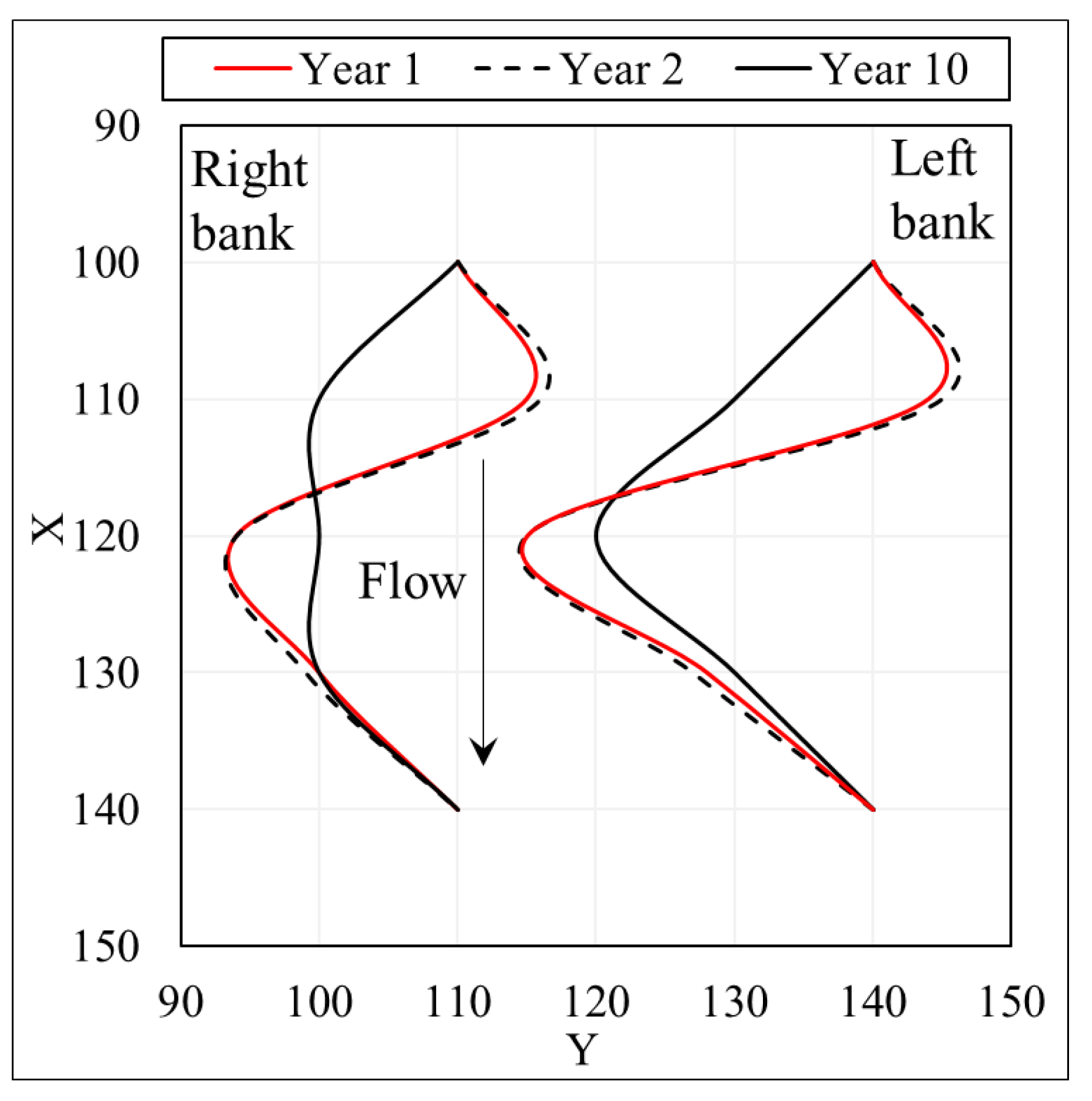
Bank lines of the Fusion River delineated from satellite images of different years (Figure A1) show that minor changes happened between Years 1 and 2 but the change is significant by Year 10. Therefore, Years 1 and 2 are in the same time window but Year 10 is in a separate time window. For generating river bathymetry relevant to the most recent planform, Year 10 is chosen as the time window for this example. It demonstrates the analysis of bank line shifting from satellite image is a convenient way to determine the time window without requiring any field data.
Figure A1. Bank lines (top view) for Fusion River delineated from satellite images.
Remotesensing 12 02799 g0a1

Appendix A.2. Input Data Processing
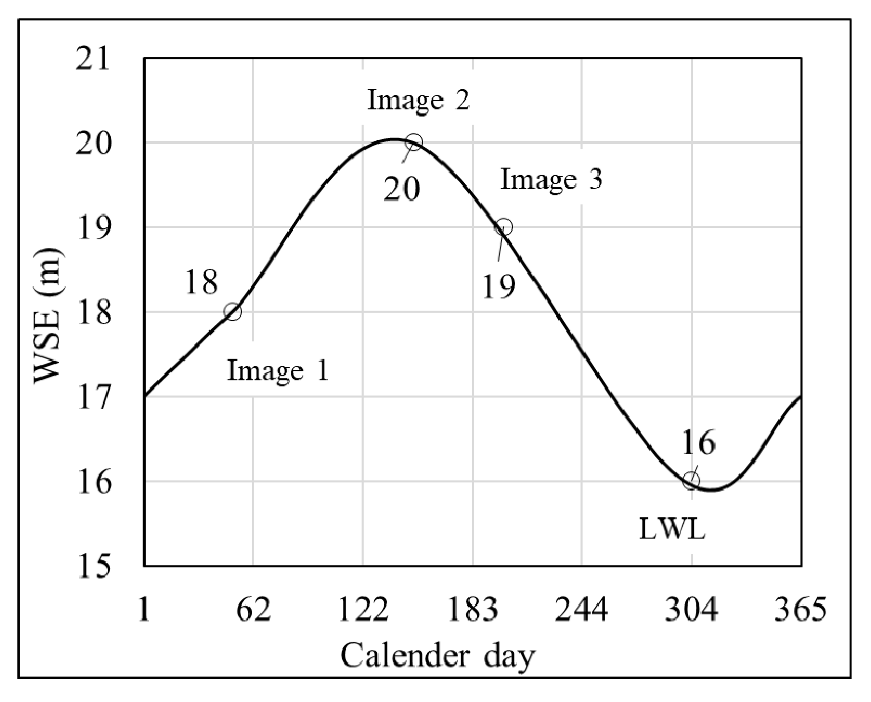
Three images within the selected time window (i.e., Year 10) is found from a source that has 10 m spatial resolution. The WSE corresponding image acquisition dates, historic hydrograph, and LWL (16 m) are presented in Figure A2.
Figure A2. Hydrograph for Fusion River and WSE corresponding to satellite image acquisition date.
Remotesensing 12 02799 g0a2
The river polygon is converted to a raster (spatial resolution 10 m) and then to river point shapefile. The river polygon, raster grids, river points, and the cell ID for the river points are presented in Figure A3.
Figure A3. (a) River polygon, (b) river raster, (c) river points, and (d) unique cell ID for the river points.
Remotesensing 12 02799 g0a3
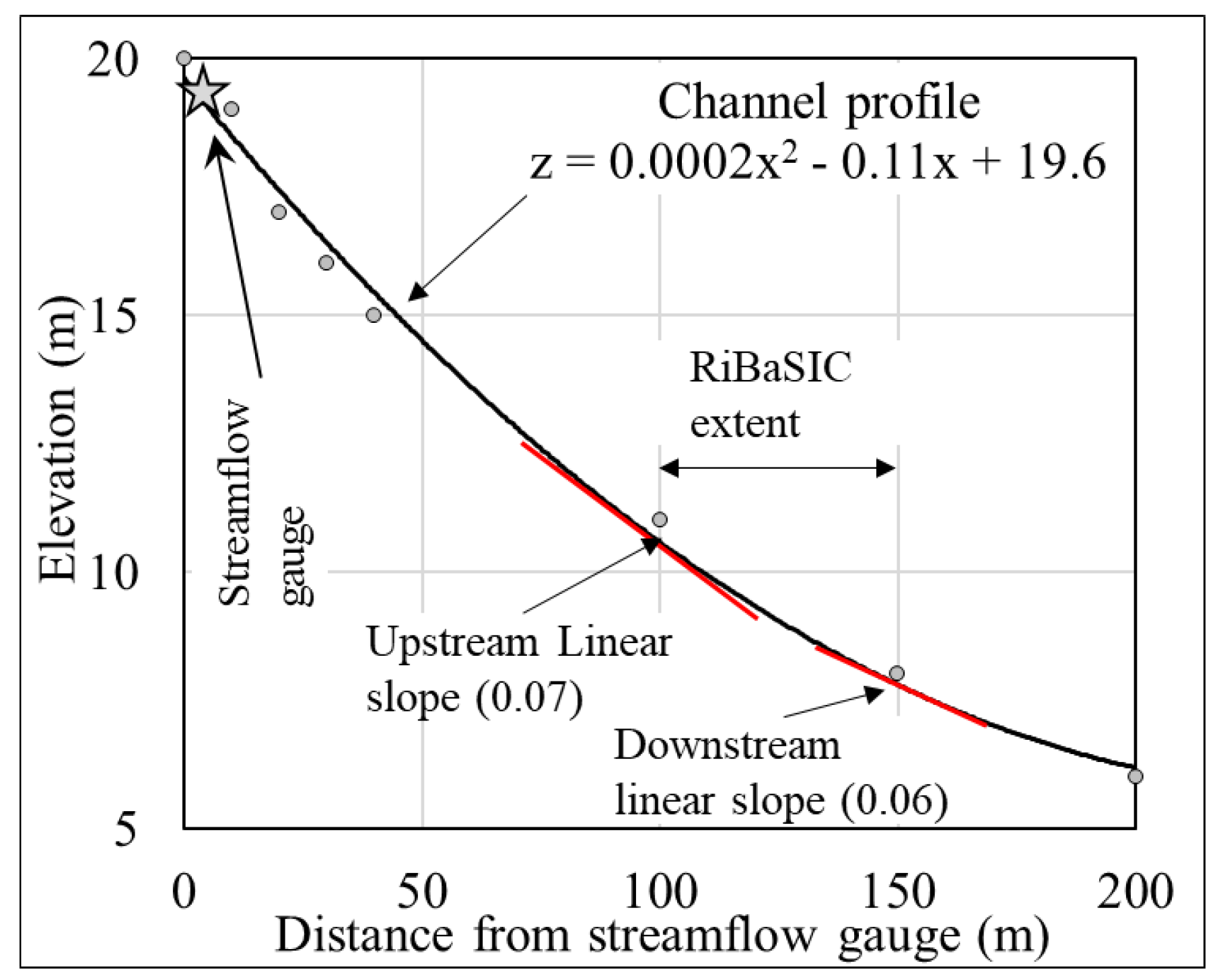
A longitudinal channel profile of the river is also determined using the DEM and shown in Figure A4.
Figure A4. Longitudinal channel profile and linear slopes at upstream and downstream of RiBaSIC extent.
Remotesensing 12 02799 g0a4

Appendix A.3. Shoreline Delineation

As mentioned in Section 2.1.3, the wet pixels in three images are determined using NDWI and the shoreline elevations are calculated. For example, cell ID 7 (third column from the left in the second row) is wet in all three images; hence, the shoreline elevation is the smallest WSE at which it is wet which is 18 m. NDWI for wet pixels in the selected images and resulting shoreline elevation for cells from three images are shown in Figure A5.
Figure A5. Normalized Difference Water Index (NDWI) for wet pixels in the selected images and shoreline elevations.
Remotesensing 12 02799 g0a5

Appendix A.4. Bathymetry Prediction

The steps of river bathymetry prediction using ADWI and WSE is presented here.
  • Image Processing: the ADWI values for channel cells in three images are shown in Figure A6.
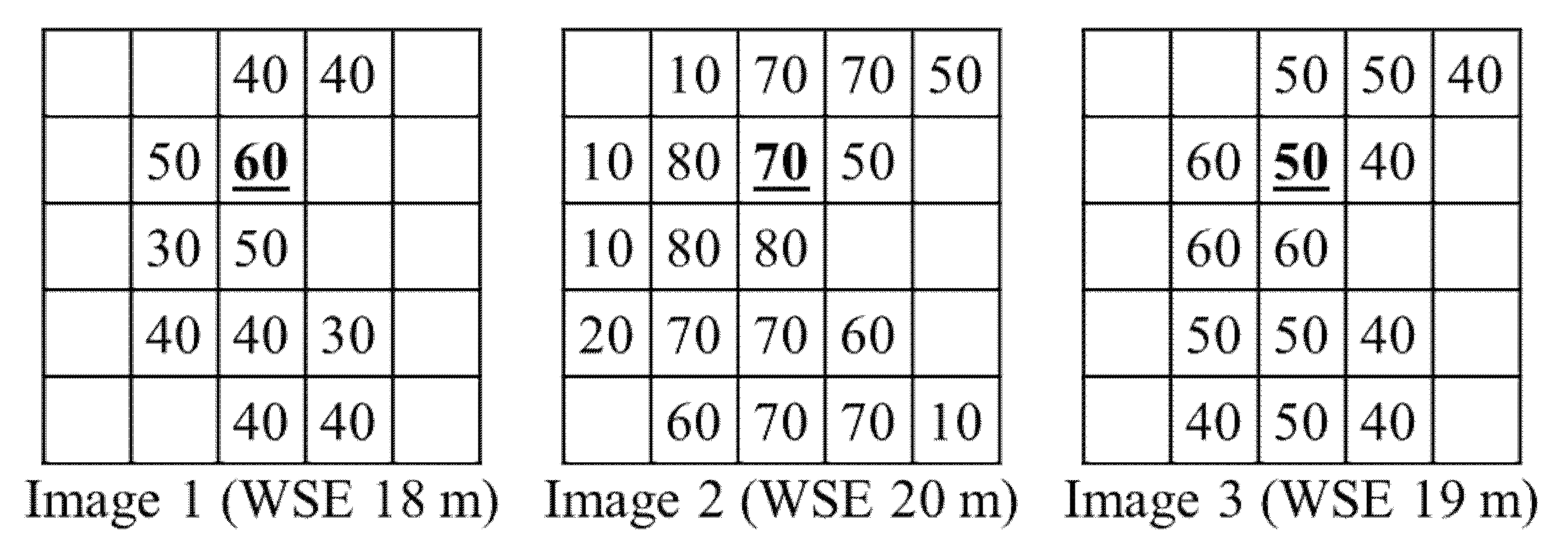
Figure A6. Average Difference Water Index (ADWI) for channel cells in the selected images.
Remotesensing 12 02799 g0a6
b.
Generating Library of ADWI and WSE: the HWSE, LWSE, DWSE, and LWI is calculated in this step are presented in Figure A7.
For cell ID number 7, from image processing:
the highest WSE at which it is in the channel is 20 m, therefore, HWSE = 20 m;
the lowest WSE at which it is in the channel is 18 m, therefore, LWSE = 18 m;
the cell is not found dry in any image, therefore, DWSE = null;
ADWI at 18 m WSE is 60, therefore, LWI = 60.
Figure A7. Lowest water surface elevation (WSE) at which a cell is found to be within a channel (LWSE), highest WSE at which a cell is found to be within a channel (HWSE), highest WSE at which a cell is found to be dry (DWSE), and low water index (LWI) for the cells calculated from ADWI.
Remotesensing 12 02799 g0a7
c.
ADWI versus Depth Correlation:
1st Trial
  • Zt = LWL = 16 (see Figure A1)
  • Therefore, depth factor, f = 20 16 20 18 = 2
  • For cell ID 7,
  • HWSE − LWSE = 2
  • Factored depth, df = f × (HWSE − LWSE) = 2 × 2 = 4 m
  • Approximate bed elevation = 20 − 4 = 16 m
  • Hence, depth in Image 1 = 18 − 16 = 2 m
  • Depth in Image 2 = 20 − 16 = 4 m
  • Depth in Image 3 = 19 − 16 = 3 m
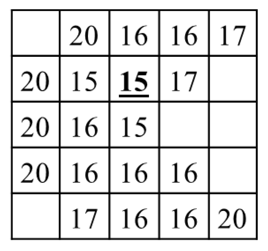
  • The factored depth (df) and approximate bed elevation for the cells are presented in Figure A8 and depth in individual images are shown in Figure A9.
Figure A8. (a) Factored depth [df] and (b) approximate bed elevation.
Remotesensing 12 02799 g0a8
Figure A9. Depth in Images 1–3 corresponding to the approximate bed elevation.
Remotesensing 12 02799 g0a9
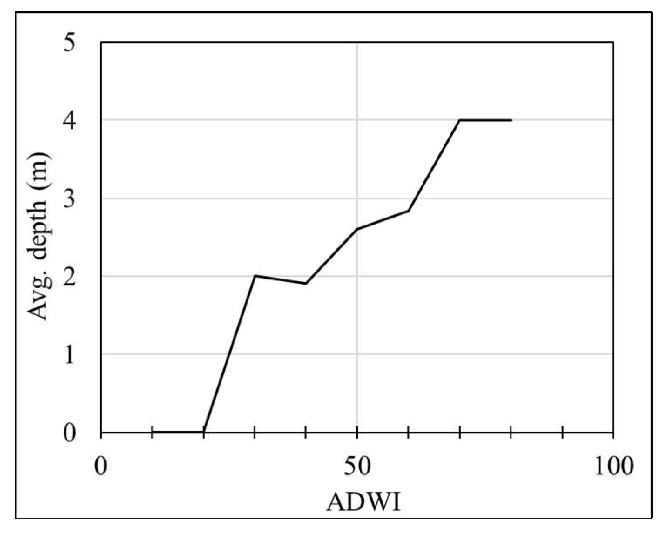
The ADWI versus average depth values calculated from all the river points (cells) from three images is calculated and presented in Figure A10.
Figure A10. ADWI versus depth correlation.
Remotesensing 12 02799 g0a10
2nd Trial
  • 1 percentile of the average depth values ≈ 0 m
  • Thalweg elevation, Zt = 16 − 0 ≈ 16 m
  • Since Zt remains the same as the 1st trial, the same ADWI versus depth correlation is found after the 2nd trial.
d.
ADWI Bathymetry:
  • For cell ID 7,
  • LWSE = 18 m
  • LWI = 60
  • Average depth from ADWI versus depth correlation = 2.8 m
  • ADWI bathymetry = 18 − 2.8 = 15.2 m
Figure A11. ADWI bathymetry. Note: numbers are shown as integers for presentation purposes.
Remotesensing 12 02799 g0a11

Appendix A.5. Post-Processing

  • Slope Transferred Elevation: the shoreline elevations and ADWI bathymetry for the cells are transferred to their corresponding geographic location using the channel profile shown in Figure A4.
    • For cell ID 7,
    • Distance, x = distance of RiBaSIC upstream from streamflow gauge + distance of cell center from RiBaSIC upstream = 100 + 15 = 115
    • Therefore, using the channel profile from Figure A4
    • Slope transferred shoreline elevation = 0.002 × 1152 − 0.11 × 115 + 18 = 8 m
    • Slope transferred ADWI bathymetry = 0.002 × 1152 − 0.11 × 115 + 15.2 = 5.2 m
    • The slope transferred cell values are presented in Figure A12.
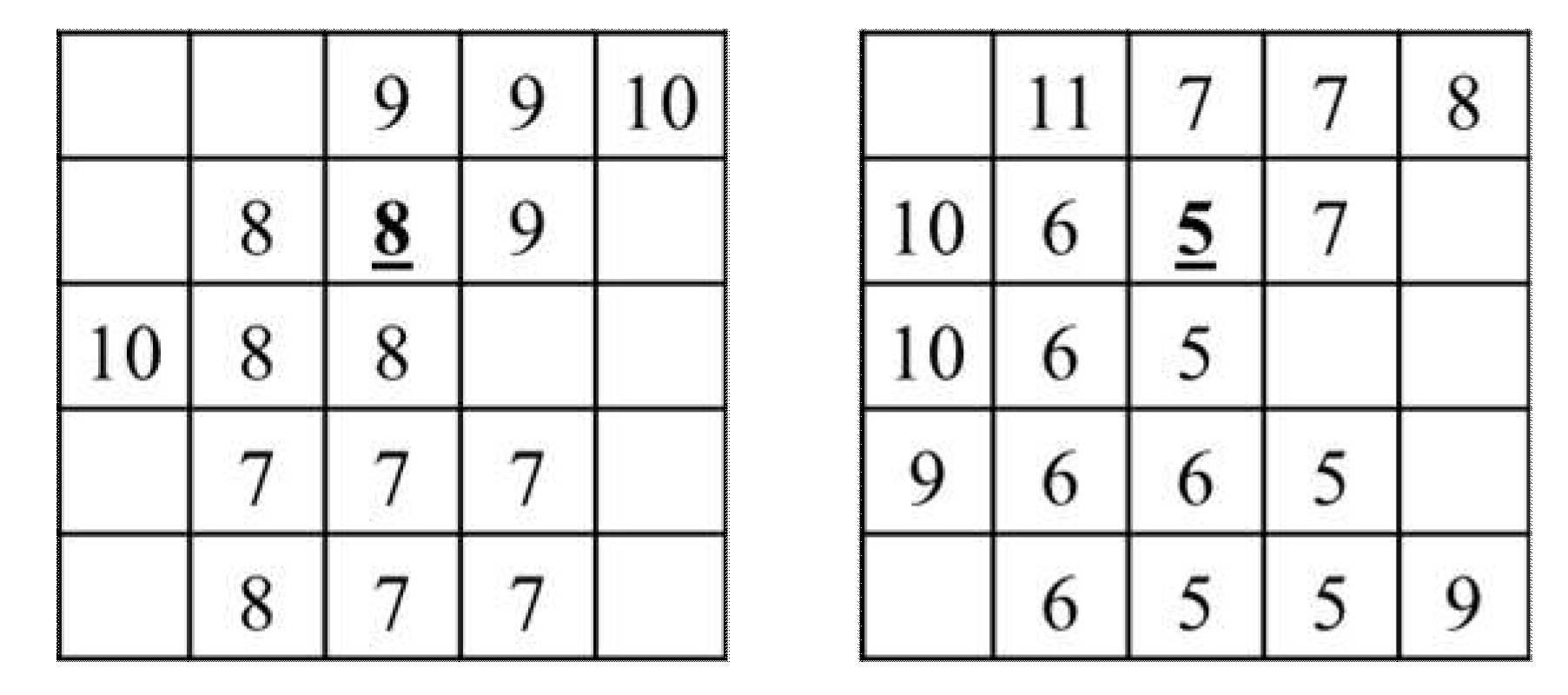
Figure A12. Slope transferred shoreline elevations (left) and ADWI bathymetry (right). Note: numbers are shown as integers for presentation purposes.
Remotesensing 12 02799 g0a12
b.
RiBaSIC Bathymetry: the main channel of the Fusion River is obtained from a dry season satellite image as shown in Figure A13. The cells inside the main channel are assigned. Slope transferred ADWI bathymetry and shoreline elevations are assigned for the cell outside of the main channel to get the RiBaSIC bathymetry as shown in Figure A13.
Cell ID 7 falls inside the main channel; therefore, ADWI bathymetry has the same elevation as slope transferred ADWI bathymetry (5 m).
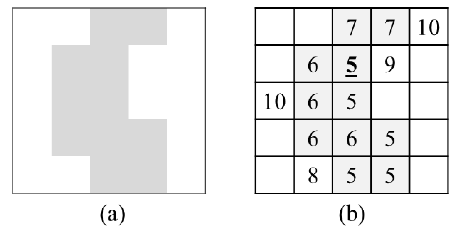
Figure A13. (a) Main channel in the dry season satellite image and (b) RiBaSIC bathymetry. Note: the cells in the main channel are shown in gray. Note: numbers are shown as integers for presentation purposes.
Remotesensing 12 02799 g0a13
c.
RiBaSIC DEM: the empty cells in RiBaSIC bathymetry are filled by elevations extracted from the DEM to produce RiBaSIC DEM as shown in Figure A14. It can be seen that for cell ID 7, the DEM elevation is 9m but that has been modified to 5 m in RiBaSIC DEM.
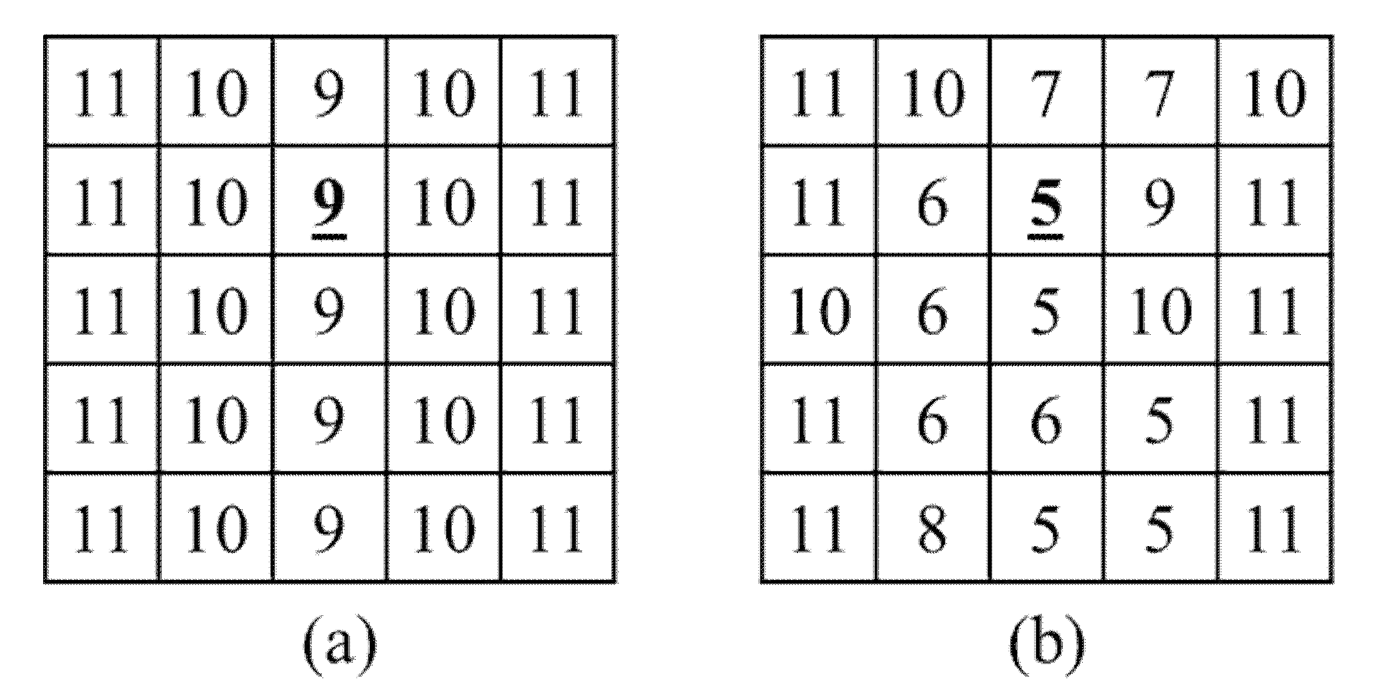
Figure A14. (a) DEM elevations and (b) RiBaSIC DEM. Note: numbers are shown as integers for presentation purposes.
Remotesensing 12 02799 g0a14
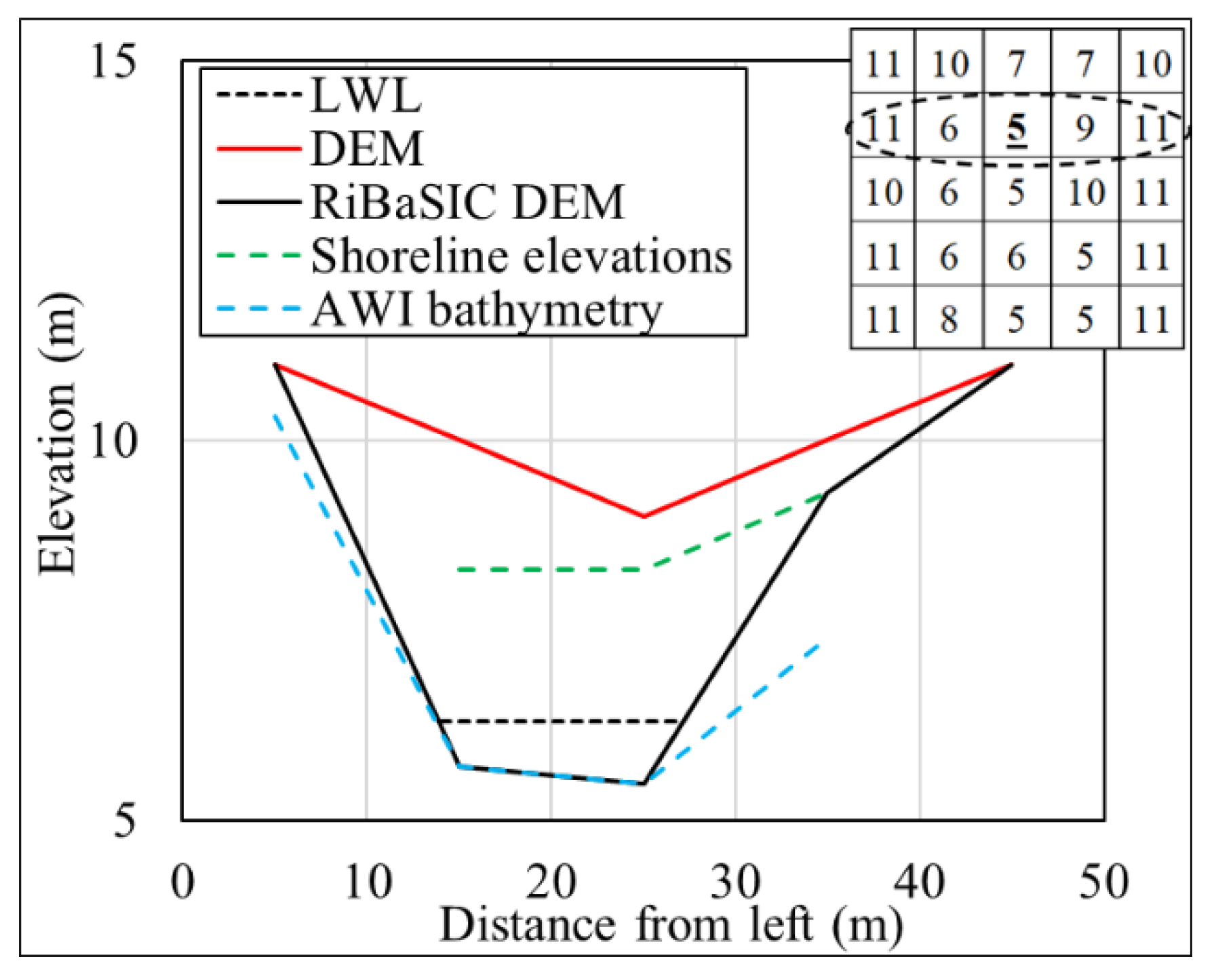
The RiBaSIC algorithm is implemented on the Fusion River for Year 10. A cross-sectional comparison at Section 2 (along row 2; shown in the dotted box) is presented in Figure A15. It can be noticed that the RiBaSIC bathymetry predicted the bed level below the LWL whereas the shoreline elevations predicted overbank areas. Therefore, RiBaSIC DEM could represent an improved channel conveyance that also reflects the planform Year 10.
Figure A15. Cross-sectional comparison of input DEM and RiBaSIC DEM along Section 2 of the Fusion River.
Remotesensing 12 02799 g0a15

References

  1. Wilson, M.; Bates, P.; Alsdorf, D.; Forsberg, B.; Horritt, M.; Melack, J.; Frappart, F.; Famiglietti, J. Modeling large-scale inundation of Amazonian seasonally flooded wetlands. Geophys. Res. Lett. 2007, 34, 15. [Google Scholar] [CrossRef] [Green Version]
  2. Bhuyian, M.; Kalyanapu, A.; Nardi, F. Approach to Digital Elevation Model Correction by Improving Channel Conveyance. J. Hydrol. Eng. 2014, 20, 04014062. [Google Scholar] [CrossRef]
  3. Kalyanapu, A.J.; Judi, D.R.; McPherson, T.N.; Burian, S.J. Annualised risk analysis approach to recommend appropriate level of flood control: Application to Swannanoa river watershed. J. Flood Risk Manag. 2015, 8, 368–385. [Google Scholar] [CrossRef]
  4. Burnham, M.; Davis, D. Effects of Data Errors on Computed Steadyâ Flow Profiles. J. Hydraul. Eng. 1990, 116, 914–929. [Google Scholar] [CrossRef]
  5. Wechsler, S.P.; Kroll, C.N. Quantifying DEM Uncertainty and its Effect on Topographic Parameters. Photogramm. Eng. Remote Sens. 2006, 72, 1081–1090. [Google Scholar] [CrossRef] [Green Version]
  6. Yamazaki, D.; Baugh, C.A.; Bates, P.D.; Kanae, S.; Alsdorf, D.E.; Oki, T. Adjustment of a spaceborne DEM for use in floodplain hydrodynamic modeling. J. Hydrol. 2012, 436, 81–91. [Google Scholar] [CrossRef]
  7. Brandt, S.A.; Lim, N.J. Importance of river bank and floodplain slopes on the accuracy of flood inundation mapping. In Proceedings of the International Conference on Fluvial Hydraulics (River Flow 2012), San Jose, Costa Rica, 5–7 September 2012; CRC Press/Balkema: Leiden, The Netherlands, 2012; pp. 1015–1020. [Google Scholar]
  8. Fisher, G.B.; Bookhagen, B.; Amos, C.B. Channel planform geometry and slopes from freely available high-spatial resolution imagery and DEM fusion: Implications for channel width scalings, erosion proxies, and fluvial signatures in tectonically active landscapes. Geomorphology 2013, 194, 46–56. [Google Scholar] [CrossRef]
  9. Jung, H.C.; Jasinski, M.F. Sensitivity of a floodplain hydrodynamic model to satellite-based DEM scale and accuracy: Case study—The Atchafalaya Basin. Remote Sens. 2015, 7, 7938. [Google Scholar] [CrossRef] [Green Version]
  10. Casas, A.; Benito, G.; Thorndycraft, V.R.; Rico, M. The topographic data source of digital terrain models as a key element in the accuracy of hydraulic flood modelling. Earth Surf Process Landf. 2006, 31, 444–456. [Google Scholar] [CrossRef]
  11. Ettritch, G.; Hardy, A.; Bojang, L.; Cross, D.; Bunting, P.; Brewer, P. Enhancing digital elevation models for hydraulic modelling using flood frequency detection. Remote Sens. Environ. 2018, 217, 506–522. [Google Scholar] [CrossRef]
  12. Mason, D.C.; Trigg, M.; Garcia-Pintado, J.; Cloke, H.L.; Neal, J.C.; Bates, P.D. Improving the TanDEM-X Digital Elevation Model for flood modelling using flood extents from Synthetic Aperture Radar images. Remote Sens. Environ. 2016, 173, 15–28. [Google Scholar] [CrossRef] [Green Version]
  13. Yamazaki, D.; Ikeshima, D.; Tawatari, R.; Yamaguchi, T.; O’Loughlin, F.; Neal, J.C.; Sampson, C.C.; Kanae, S.; Bates, P.D. A high-accuracy map of global terrain elevations. Geophys. Res. Lett. 2017, 44, 5844–5853. [Google Scholar] [CrossRef] [Green Version]
  14. Bogoni, M.; Putti, M.; Lanzoni, S. Modeling meander morphodynamics over self-formed heterogeneous floodplains. Water Resour. Res. 2017, 53, 5137–5157. [Google Scholar] [CrossRef] [Green Version]
  15. Downward, S.; Gurnell, A.; Brookes, A. A methodology for quantifying river channel planform change using GIS. IAHS Publ. Ser. Proc. Rep. Intern Assoc. Hydrol. Sci. 1994, 224, 449–456. [Google Scholar]
  16. Maswood, M.; Hossain, F. Advancing river modelling in ungauged basins using satellite remote sensing: The case of the Ganges-Brahmaputra-Meghna basin. Int. J. River Basin Manag. 2016, 14, 103–117. [Google Scholar] [CrossRef]
  17. Schaperow, J.R.; Li, D.; Margulis, S.A.; Lettenmaier, D.P. A curve-fitting method for estimating bathymetry from water surface height and width. Water Resour. Res. 2019, 55, 4288–4303. [Google Scholar] [CrossRef]
  18. Gichamo, T.Z.; Popescu, I.; Jonoski, A.; Solomatine, D. River cross-section extraction from the ASTER global DEM for flood modeling. Environ. Model. Softw. 2012, 31, 37. [Google Scholar] [CrossRef]
  19. Merwade, V.; Maidment, D.R. A GIS Framework for Describing River Channel Bathymetry; University of Texas at Austin, Center for Research in Water Resources, JJ Pickle Research Campus: Austin, TX, USA, 2004. [Google Scholar]
  20. Wood, M.; Hostache, R.; Neal, J.; Wagener, T.; Giustarini, L.; Chini, M.; Corato, G.; Matgen, P.; Bates, P. Calibration of channel depth and friction parameters in the LISFLOOD-FP hydraulic model using medium-resolution SAR data and identifiability techniques. Hydrol. Earth Syst. Sci. 2016, 20, 4983–4997. [Google Scholar] [CrossRef] [Green Version]
  21. Neal, J.C.; Odoni, N.A.; Trigg, M.A.; Freer, J.E.; Garcia-Pintado, J.; Mason, D.C.; Wood, M.; Bates, P.D. Efficient incorporation of channel cross-section geometry uncertainty into regional and global scale flood inundation models. J. Hydrol. 2015, 529, 169–183. [Google Scholar] [CrossRef] [Green Version]
  22. Lim, N.J.; Brandt, S.A. Flood map boundary sensitivity due to combined effects of DEM resolution and roughness in relation to model performance. Geomat. Nat. Hazards Risk 2019, 10, 1613–1647. [Google Scholar] [CrossRef] [Green Version]
  23. Bizzi, S.; Demarchi, L.; Grabowski, R.C.; Weissteiner, C.J.; van de Bund, W. The use of remote sensing to characterise hydromorphological properties of European rivers. Aquat. Sci. 2016, 78, 57–70. [Google Scholar] [CrossRef] [Green Version]
  24. Legleiter, C.J. Calibrating remotely sensed river bathymetry in the absence of field measurements: Flow REsistance Equation-Based Imaging of River Depths (FREEBIRD). Water Resour. Res. 2015, 51, 2865–2884. [Google Scholar] [CrossRef]
  25. Legleiter, C. Mapping river depth from publicly available aerial images. River Res. Appl. 2013, 29, 760–780. [Google Scholar] [CrossRef]
  26. Legleiter, C.J. Remote measurement of river morphology via fusion of LiDAR topography and spectrally based bathymetry. Earth Surf Process Landf. 2012, 37, 499–518. [Google Scholar] [CrossRef]
  27. Marcus, W.A.; Fonstad, M.A. Remote sensing of rivers: The emergence of a subdiscipline in the river sciences. Earth Surf Process Landf. 2010, 35, 1867–1872. [Google Scholar] [CrossRef]
  28. Legleiter, C.J.; Roberts, D.A.; Lawrence, R.L. Spectrally based remote sensing of river bathymetry. Earth Surf Process Landf. 2009, 34, 1039–1059. [Google Scholar] [CrossRef]
  29. Fonstad, M.A.; Marcus, W.A. Remote sensing of stream depths with hydraulically assisted bathymetry (HAB) models. Geomorphology 2005, 72, 320–339. [Google Scholar] [CrossRef]
  30. Legleiter, C.J. Inferring river bathymetry via image-to-depth quantile transformation (IDQT). Water Resour. Res. 2016, 52, 3722–3741. [Google Scholar] [CrossRef] [Green Version]
  31. Moramarco, T.; Barbetta, S.; Bjerklie, D.M.; Fulton, J.W.; Tarpanelli, A. River Bathymetry Estimate and Discharge Assessment from Remote Sensing. Water Resour. Res. 2019, 55, 6692–6711. [Google Scholar] [CrossRef]
  32. Dey, S.; Saksena, S.; Merwade, V. Assessing the effect of different bathymetric models on hydraulic simulation of rivers in data sparse regions. J. Hydrol. 2019, 575, 838–851. [Google Scholar] [CrossRef]
  33. McCabe, M.F.; Rodell, M.; Alsdorf, D.E.; Miralles, D.G.; Uijlenhoet, R.; Wagner, W.; Lucieer, A.; Houborg, R.; Verhoest, N.E.; Franz, T.E. The future of Earth observation in hydrology. Hydrol. Earth Syst. Sci. 2017, 21, 3879. [Google Scholar] [CrossRef] [PubMed] [Green Version]
  34. Biancamaria, S.; Lettenmaier, D.P.; Pavelsky, T.M. The SWOT mission and its capabilities for land hydrology. In Remote Sensing and Water Resources; Springer: Berlin/Heidelberg, Germany, 2016; pp. 117–147. [Google Scholar]
  35. Bhuyian, M.N.; Kalyanapu, A. Predicting Channel Conveyance in the Obion River Watershed Using SAMBLE Method. J. Hydrol. Eng. 2020, 25, 05019033. [Google Scholar] [CrossRef]
  36. Khan, M.J.U.; Ansary, M.; Durand, F.; Testut, L.; Ishaque, M.; Calmant, S.; Krien, Y.; Islam, A.; Papa, F. High-Resolution Intertidal Topography from Sentinel-2 Multi-Spectral Imagery: Synergy between Remote Sensing and Numerical Modeling. Remote Sens. 2019, 11, 2888. [Google Scholar] [CrossRef] [Green Version]
  37. Bergmann, M.; Durand, F.; Krien, Y.; Khan, M.J.U.; Ishaque, M.; Testut, L.; Calmant, S.; Maisongrande, P.; Islam, A.S.; Papa, F. Topography of the intertidal zone along the shoreline of Chittagong (Bangladesh) using PROBA-V imagery. Int. J. Remote Sens. 2018, 39, 9004–9024. [Google Scholar] [CrossRef]
  38. Mason, D.; Davenport, I.; Flather, R. Interpolation of an intertidal digital elevation model from heighted shorelines: A case study in the western Wash. Oceanogr. Lit. Rev. 1998, 7, 1102–1103. [Google Scholar] [CrossRef]
  39. Wang, Y.; Koopmans, B. Mapping and monitoring the tidal flats of coastal areas on basis of sequential ERS SAR. In Proceedings of the Second ERS Applications Workshop, London, UK, 6–8 December 1996; pp. 343–347. [Google Scholar]
  40. Mason, D.; Davenport, I.; Robinson, G.; Flather, R.; McCartney, B. Construction of an inter-tidal digital elevation model by the ‘Water-Line’Method. Geophys. Res. Lett. 1995, 22, 3187–3190. [Google Scholar] [CrossRef]
  41. McFeeters, S.K. The use of the Normalized Difference Water Index (NDWI) in the delineation of open water features. Int. J. Remote Sens. 1996, 17, 1425–1432. [Google Scholar] [CrossRef]
  42. Zhu, Z.; Wang, S.; Woodcock, C.E. Improvement and expansion of the Fmask algorithm: Cloud, cloud shadow, and snow detection for Landsats 4–7, 8, and Sentinel 2 images. Remote Sens. Environ. 2015, 159, 269–277. [Google Scholar] [CrossRef]
  43. Zhu, Z.; Woodcock, C.E. Object-based cloud and cloud shadow detection in Landsat imagery. Remote Sens. Environ. 2012, 118, 83–94. [Google Scholar] [CrossRef]
  44. Polidorio, A.M.; Flores, F.C.; Franco, C.; Imai, N.N.; Tommaselli, A.M. Enhancement of terrestrial surface features on high spatial resolution multispectral aerial images. In Proceedings of the IEEE 23rd SIBGRAPI Conference on Graphics, Patterns and Images, Gramado, Brazil, 30 August–3 September 2010; pp. 295–300. [Google Scholar]
  45. Woldai, T. Electromagnetic energy and remote sensing. In Principles of Remote Sensing: An Introductory Textbook; International Institute for Geo-Information Science and Earth Observation: Enschede, The Netherlands, 2004; pp. 29–38. [Google Scholar]
  46. Lacey, G. A general theory of flow in alluvium. J. Inst. Civ. Eng. 1946, 27, 16–47. [Google Scholar] [CrossRef]
  47. Bray, D.I. Estimating average velocity in gravel-bed rivers. J. Hydraul. Div. 1979, 105, 1103–1122. [Google Scholar]
  48. Coon, W.F. Estimation of Roughness Coefficients for Natural Stream Channels with Vegetated Banks; US Geological Survey: Reston, VA, USA, 1998.
  49. Lang, S.; Ladson, T.; Anderson, B. A review of empirical equations for estimating stream roughness and their application to four streams in Victoria. Australas. J. Water Resour. 2004, 8, 69–82. [Google Scholar] [CrossRef]
  50. Jarrett, R.D. Hydraulics of high-gradient streams. J. Hydraul. Eng. 1984, 110, 1519–1539. [Google Scholar] [CrossRef]
  51. Te Chow, V. Open-Channel Hydraulics; McGraw-Hill: New York, NY, USA, 1959. [Google Scholar]
  52. LeFavour, G.; Alsdorf, D. Water slope and discharge in the Amazon River estimated using the shuttle radar topography mission digital elevation model. Geophys. Res. Lett. 2005, 32. [Google Scholar] [CrossRef] [Green Version]
  53. Hall, A.C.; Schumann, G.J.; Bamber, J.L.; Bates, P.D.; Trigg, M.A. Geodetic corrections to Amazon River water level gauges using ICESat altimetry. Water Resour. Res. 2012, 48, 6. [Google Scholar] [CrossRef] [Green Version]
  54. FAP24. River Survey Project Annex 3: Hydrology; Final Report; Water Resources Planning Organization: Dhaka, Bangladesh, 1996.
  55. Lind, G.D.; Wellman, R.E.; Mangano, J.F. Boat-Based River Bathymetry and Stream Velocity on the Upper Willamette River, Oregon, Spring 2015; U.S. Geological Survey: Reston, VA, USA, 2017. [CrossRef]
  56. Bjerklie, D.M.; Moller, D.; Smith, L.C.; Dingman, S.L. Estimating discharge in rivers using remotely sensed hydraulic information. J. Hydrol. 2005, 309, 191–209. [Google Scholar] [CrossRef]
  57. Brombacher, J.; Reiche, J.; Dijksma, R.; Teuling, A.J. Near-daily discharge estimation in high latitudes from Sentinel-1 and 2: A case study for the Icelandic Þjórsá river. Remote Sens. Environ. 2020, 241, 111684. [Google Scholar] [CrossRef]
  58. Feng, D.; Gleason, C.J.; Yang, X.; Pavelsky, T.M. Comparing discharge estimates made via the BAM algorithm in high-order Arctic rivers derived solely from optical CubeSat, Landsat, and Sentinel-2 data. Water Resour. Res. 2019, 55, 7753–7771. [Google Scholar] [CrossRef]
  59. Kim, D.; Yu, H.; Lee, H.; Beighley, E.; Durand, M.; Alsdorf, D.E.; Hwang, E. Ensemble learning regression for estimating river discharges using satellite altimetry data: Central Congo River as a Test-bed. Remote Sens. Environ. 2019, 221, 741–755. [Google Scholar] [CrossRef]
  60. Bogning, S.; Frappart, F.; Blarel, F.; Niño, F.; Mahé, G.; Seyler, F.; Braun, J.; Onguéné, R.; Etamé, J. Estimating River Discharges in the Ogooue River Basin Using Satellite Altimetry Data. In Proceedings of the 2018 IEEE International Geoscience and Remote Sensing Symposium (IGARSS 2018), Valencia, Spain, 22–27 July 2018; pp. 9304–9307. [Google Scholar]
  61. Sichangi, A.; Wang, L.; Hu, Z. Estimation of River Discharge Solely from Remote-Sensing Derived Data: An Initial Study Over the Yangtze River. Remote Sens. 2018, 10, 1385. [Google Scholar] [CrossRef] [Green Version]
  62. Tarpanelli, A.; Santi, E.; Tourian, M.J.; Filippucci, P.; Amarnath, G.; Brocca, L. Daily river discharge estimates by merging satellite optical sensors and radar altimetry through artificial neural network. IEEE Trans. Geosci. Remote Sens. 2018, 57, 329–341. [Google Scholar] [CrossRef]
  63. Oubanas, H.; Gejadze, I.; Malaterre, P.; Durand, M.; Wei, R.; Frasson, R.P.; Domeneghetti, A. Discharge estimation in ungauged basins through variational data assimilation: The potential of the SWOT mission. Water Resour. Res. 2018, 54, 2405–2423. [Google Scholar] [CrossRef]
  64. Durand, M.; Gleason, C.; Garambois, P.; Bjerklie, D.; Smith, L.; Roux, H.; Rodriguez, E.; Bates, P.D.; Pavelsky, T.M.; Monnier, J. An intercomparison of remote sensing river discharge estimation algorithms from measurements of river height, width, and slope. Water Resour. Res. 2016, 52, 4527–4549. [Google Scholar] [CrossRef] [Green Version]
  65. Tourian, M.; Tarpanelli, A.; Elmi, O.; Qin, T.; Brocca, L.; Moramarco, T.; Sneeuw, N. Spatiotemporal densification of river water level time series by multimission satellite altimetry. Water Resour. Res. 2016, 52, 1140–1159. [Google Scholar] [CrossRef] [Green Version]
  66. Bhuyian, M.N.; Kalyanapu, A. Accounting digital elevation uncertainty for flood consequence assessment. J. Flood Risk Manag. 2018, 11, S1051–S1062. [Google Scholar] [CrossRef]
  67. Andreadis, K.M.; Clark, E.A.; Lettenmaier, D.P.; Alsdorf, D.E. Prospects for river discharge and depth estimation through assimilation of swath-altimetry into a raster-based hydrodynamics model. Geophys. Res. Lett. 2007, 34, 10. [Google Scholar] [CrossRef] [Green Version]
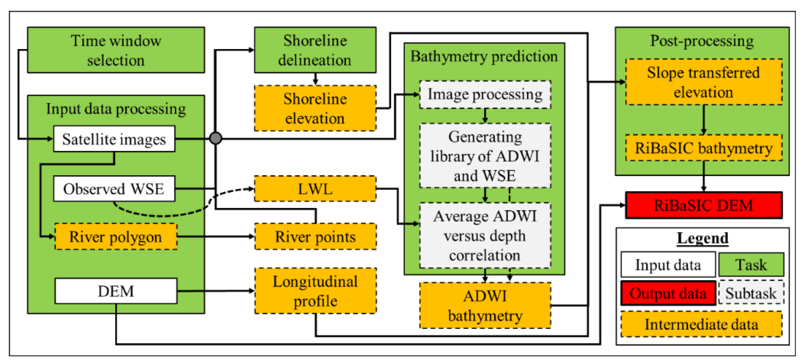
Figure 1. Flowchart of the River Bathymetry via Satellite Image Compilation (RiBaSIC) algorithm. Note: Details of the tasks are presented in Section 2.1 and a list of acronyms is provided in Abbreviations.
Remotesensing 12 02799 g001
Figure 2. Post-processing of RiBaSIC to produce the RiBaSIC Digital Elevation Model (DEM).
Remotesensing 12 02799 g002
Figure 3. Flowchart of Manning’s roughness factor approximation methodology.
Remotesensing 12 02799 g003
Figure 4. RiBaSIC extent (shown in solid black), hydrodynamic (HD) model extent (shown in cross-hatch), nearby streamflow gauges, and location of cross-section surveys (shown in red) in the study areas.
Remotesensing 12 02799 g004
Figure 5. Planform view of RiBaSIC bathymetry in some reaches SA1 (Willamette River), SA2 (Kushiyara River), SA3 (Jamuna River), and SA4 (Solimoes River). Note: SRTM waterbody data (presented in dotted lines) represents the planform of the year 2000.
Remotesensing 12 02799 g005
Figure 6. Comparison of surveyed river cross-sections with SRTM, MERIT, and RiBaSIC bathymetry derived cross-sections in SA1 (a,b), SA2 (c,d), SA3 (e,f), and SA4 (g).
Remotesensing 12 02799 g006
Figure 7. Observed and modeled hydrographs for SA1, SA2, SA3, and SA4; the discharge in the vertical axis is shown in a thousand m3.
Remotesensing 12 02799 g007
Table 1. Equations for estimating Manning’s roughness factors from morphological properties.
EquationMethodFormulaSourceRemarks
9Lacey (1946) n = 0.0928 S 1 / 6 [46]R = Hydraulic radius (ft)
S = Channel slope
Sw = Slope of water surface
Sf = Energy gradient
10Bray (1979) n = 0.104 S W 0.177 [47,48]
11Bray (1982) n = 1 8 S W 0.21 R 0.067 [49]
12Jarrett (1984) n = 0.39 S f 0.38 R 0.16 [50]
13Sauer (1990) n = 0.11 S W 0.18 R 0.08 [48,49]
Table 2. Description of the study areas and data.
Study AreaSA1SA2SA3SA4
RiverWillamette Kushiyara Jamuna Solimoes
BasinColumbiaMeghnaBrahmaputraAmazon
CountryUSABangladeshBangladeshBrazil
River characteristicsPlanformMeanderingMeanderingBraidedWandering
Top width (m)12020012,0007000
Tidal effectNoNoNoNo
SeasonDryJul–NovJan–MayJan–MayAug–Dec
WetDec–JunJun–DecJun–DecJan–Jul
ExtentRiBaSICHarrisburg to Albany (67 km)Fenchuganj to Markuli (80 km)Kazipur (25 km)Iranduba (15 km)
HD modelHarrisburg to Corvallis (47 km)Fenchuganj to Monu confluence (32 km)
PeriodRiBaSIC2013–20152000–200220102010
HD model2009–20132001–20052009–20132009–2013
HD modelGrid size (m)30 × 3030 × 30100 × 100100 × 100
Time step (s)300300300300
Satellite ImageLandsat 7, 85, 75, 75, 7
Count129672930
DEMSlope estimationSRTMSRTMSRTM1 [52]
FloodplainMERITMERITMERITMERIT
WSELocationHarrisburgFenchuganjBahadurabad2 Manacapuru
SourceUSGSBWDBBWDB2 SO-HYBAM
DischargeLocationHarrisburgSherpurBahadurabadManacapuru
SourceUSGSBWDB3FAP24HYBAM
Bathymetric surveyPeriod2015200420114 N/A
Source5 USGSBWDBBWDB4 Brazil Navy
Slope (upstream–downstream)RiBaSIC0.0009–0.00020.00006–0.0000050.000080.000019
1 The linear slope at Manacapuru is estimated from SRTM [52]. 2 WSE at Manacapuru is adjusted by 3.54 m offset to match with Earth Gravitational Model 1996 (EGM96) Geoid [53]. 3 Daily discharge at Bahadurabad is calculated using a published rating curve [54]. 4 The date of the bathymetric survey is not mentioned in the navigation chart. 5 Bathymetry survey conducted by USGS for NASA SWOT mission [55] is merged with LiDAR DEM from the Oregon Department of Geology and Mineral Industries (DOGAMI). Note: Please refer to Abbreviations for a list of acronyms.
Table 3. Manning’s n approximation and performance of model simulations for the study areas.
IDSA1SA2SA3SA4
RiverWillametteKushiyaraJamunaSolimoes
LocationHarrisburgMonu confluenceKazipurIranduba
Streamflow gaugeHarrisburgSherpurBahadurabadManacapuru
SlopeUpstream0.00090.0000590.000080.000019
Downstream0.00040.0000560.000080.000019
Hydraulic Radius (m)Upstream3.757.474.0417.33
Downstream3.297.394.0417.33
Manning’s n (upstream)Lacey (1946)0.0290.0180.0190.015
Bray (1979)0.0300.0190.0200.015
Bray (1982)0.0340.0200.0200.017
Jarrett (1984)0.0180.0060.0070.003
Sauer (1990)0.0380.0250.0250.021
Average0.0300.0200.0210.017
Manning’s n (downstream)Lacey (1946)0.0250.0180.0190.015
Bray (1979)0.0260.0180.0200.015
Bray (1982)0.0280.0200.0200.017
Jarrett (1984)0.0130.0060.0070.003
Sauer (1990)0.0320.0240.0250.021
Average0.0250.0200.0210.017
RRMSEDry11%19%25%21%
Wet17%17%16%10%
Annual17%19%19%14%
NSE0.970.950.980.93
Correlation coefficient0.980.990.980.98