Construction of the Long-Term Global Surface Water Extent Dataset Based on Water-NDVI Spatio-Temporal Parameter Set


1
State Key Laboratory of Remote Sensing Science, Aerospace Information Research Institute, Chinese Academy of Sciences, Beijing 100094, China
2
School of Electronic, Electrical and Communication Engineering, University of Chinese Academy of Sciences, Beijing 100049, China
*
Author to whom correspondence should be addressed.
Remote Sens. 2020, 12(17), 2675; https://doi.org/10.3390/rs12172675
Submission received: 6 July 2020
/
Revised: 12 August 2020
/
Accepted: 17 August 2020
/
Published: 19 August 2020
(This article belongs to the Section Remote Sensing in Geology, Geomorphology and Hydrology)
Abstract
:Inland surface water is highly dynamic, seasonally and inter-annually, limiting the representativity of the water coverage information that is usually obtained at any single date. The long-term dynamic water extent products with high spatial and temporal resolution are particularly important to analyze the surface water change but unavailable up to now. In this paper, we construct a global water Normalized Difference Vegetation Index (NDVI) spatio-temporal parameter set based on the Moderate-resolution Imaging Spectroradiometer (MODIS) NDVI. Employing the Google Earth Engine, we construct a new Global Surface Water Extent Dataset (GSWED) with coverage from 2000 to 2018, having an eight-day temporal resolution and a spatial resolution of 250 m. The results show that: (1) the MODIS NDVI-based surface water mapping has better performance compared to other water extraction methods, such as the normalized difference water index, the modified normalized difference water index, and the OTSU (maximal between-cluster variance method). In addition, the water-NDVI spatio-temporal parameter set can be used to update surface water extent datasets after 2018 as soon as the MODIS data are updated. (2) We validated the GSWED using random water samples from the Global Surface Water (GSW) dataset and achieved an overall accuracy of 96% with a kappa coefficient of 0.9. The producer’s accuracy and user’s accuracy were 97% and 90%, respectively. The validated comparisons in four regions (Qinghai Lake, Selin Co Lake, Utah Lake, and Dead Sea) show a good consistency with a correlation value of above 0.9. (3) The maximum global water area reached 2.41 million km2 between 2000 and 2018, and the global water showed a decreasing trend with a significance of P = 0.0898. (4) Analysis of different types of water area change regions (Selin Co Lake, Urmia Lake, Aral Sea, Chiquita Lake, and Dongting Lake) showed that the GSWED can not only identify the seasonal changes of the surface water area and abrupt changes of hydrological events but also reflect the long-term trend of the water changes. In addition, GSWED has better performance in wetland areas and shallow areas. The GSWED can be used for regional studies and global studies of hydrology, biogeochemistry, and climate models.

1. Introduction
Surface water plays an important role in the terrestrial water cycle and ecosystem balance. It not only provides social, economic, and environmental services but also provides significant resources for animals and plants. On the one hand, surface water has seasonal dynamic characteristics; on the other hand, surface water also has drastic characteristics, such as shrinkage, expansion, and shape change due to natural or human influences [1]. The spatial and temporal heterogeneity of surface water distribution affects other natural resources and even the environment and human life [2,3]. Obtaining the spatial and temporal distribution of surface water in a timely manner is important for disaster prevention (reducing floods and mitigating droughts), understanding the mechanisms and processes of water cycle changes, and responding to global changes [4,5]. The water distribution map is also an important source of information for ecosystem management and political decision-makers [3,6,7,8]. The temporal coverage and accuracy of water classifications also play a key role in bathymetry generation. By combining long-term and highly frequent water classifications and altimetry data, the bathymetry map for inland water can be generated, which is very important for many aspects of water management [9,10,11].
The above process studies require surface water datasets. So far, the global surface water datasets that have been generated can be divided into two categories: static and dynamic datasets. The spatial resolution of the static global surface water datasets ranges from 1 km to 14.25 m [12,13,14,15,16,17,18,19,20,21]. Due to the dynamics of surface water, the static water datasets cannot reflect the characteristics of surface water change. Therefore, a variety of dynamic water datasets with different temporal resolutions have been generated. One of them is the Global Inundation Extent from Multi-Satellites (GIEMS) with a temporal resolution of one month [8,22]. Considering its coarse spatial resolution, Fluet-Chouinard et al. [23] downscaled GIEMS to GIEMS-D15 with a spatial resolution of 500 m, and Aires et al. [24] downscaled GIEMS to GIEMS-D3 with a spatial resolution of 90 m. Pekel et al. [25] developed the GSW dataset based on Landsat archives over 32 years (1984–2015). Because the low temporal resolution of Landsat, the actual temporal resolution of this product cannot meet the monitoring requirements of rapid changes in surface water [25]. These global surface water datasets have great advantages in studying climate changes over a longer period. At the same time, to improve the spatial and temporal resolution of these datasets can be more significant for studying both trend analysis and annual/seasonal variability of global surface water. Ji et al. [26] produced a daily global surface water database (2001–2016) with a spatial resolution of 500 m based on a MODIS surface reflectance daily level 2G product with a spatial resolution of 500 m (MOD09GA). This database can monitor water changes with long-term sequence and high time frequency, but the spatial resolution is low, and the extraction precision for some small water bodies is poor. Klein et al. [27] also produced the daily global water surface dataset Global WaterPack (GWP) with a spatial resolution of 250 m from 2013 to 2015, which was not able to monitor water change over long-term sequence. Lu et al. [28] produced China’s eight-day 250 m surface water dataset that only covers China from 2000 to 2016 based on MOD09Q1. Policelli et al. [29] created the daily MODIS Water Product (MWP) dataset, with a spatial resolution of 250 m between 2013 and 2020. Lin et al. [30] and Tran et al. [31] used algorithms to remove cloud and shadow pixels in MWP. These datasets are committed to providing rapid mapping of water bodies in a specific area and serving more actual social needs, rather than studying the changes of global surface water over the long term and serving climate change and ecosystem researches. Though indexes such as the Normalized Difference Water Index (NDWI), the Modified Normalized Difference Water Index (MNDWI), supervised classification, or even an automation method are useful for extraction of local surface water with low temporal frequency [32,33,34,35,36,37], they are not applicable for large-scale water mapping with high spatial and temporal resolution. The spectral characteristics of surface water vary in time and space on a global scale. Differences in water depth, suspended solids, sediment content, chlorophyll concentration, and algae can cause differences in the spectral characteristics of surface water [38]. For example, a river is relatively clear under ideal conditions, but the spectral characteristics of water at shallows would mix the spectral characteristics of the bottom mud, and the Normalized Difference Vegetation Index (NDVI) of the water with mixed vegetation would be higher. Surface water in cold zones is often frozen or covered by snow or ice for most of the year; shadows of mountains and clouds are often confused with surface water. Changes in atmospheric conditions and changes of the solar elevation angle and the sensor’s viewing angle will also cause differences in the spectral characteristics of the surface water. Clouds are the most unfavorable factor of water extraction for optical images [27,38,39]. Regarding SAR data, due to the short time span, SAR-based water mapping is mostly concentrated on small areas and short time scales [40,41]. In summary, there are some limitations to existing global water datasets regarding the spatial resolution, temporal resolution, and time span.
With the rapid development of the global society and economy, surface water has undergone significant changes worldwide, with the global average maximum range of water decreasing by 6% between 1993 and 2007 [8,42]. However, surface water in various regions shows different trends. For example, in the South Aral Sea, the water decreased by more than 70% in 2001–2016 [43], while the lakes in the Qinghai–Tibet Plateau showed an overall expansion trend [44,45], and Lake Chad first increased and then decreased [46,47]. Therefore, there is clearly a need to generate a long-term global surface water extent product with high spatial and temporal resolution, which can not only depict the seasonal changes in surface water and identify the short-term sporadic hydrological events, but also can reflect the change trend of surface water. It can support us to better understand the impact of natural changes, global climate change, and human activities (such as dams, etc.) on the global water cycle.
The purpose of this research is to generate a global, long-term, reliable, and high spatial-temporal resolution surface water extent dataset (GSWED) with eight-day temporal resolution and 250 m spatial resolution. After introducing the data sources (Section 2), we propose an effective threshold method (Section 3) for large-scale surface water extraction that could be applied to most optical satellite sensors such as MODIS. In Section 4, we present the validation results and demonstrate the advantages of GSWED in capturing the different change patterns of various representative lakes across the world. We compare the method of this study with other methods, and our product with other similar products, in Section 5. The GSWED was constructed and validated by employing the Google Earth Engine (GEE) remote sensing big data cloud platform.
2. Date Sources
2.1. Datasets for Water Mapping and Validation
MODIS has moderate spatial resolution and high temporal resolution, so it is an ideal data source for extracting global surface water. The main input datasets for this study are the eight-day surface reflectance product that was composited by the daily MODIS reflectance products. Its global coverage with high temporal resolution is particularly suitable for large-scale monitoring. We used the MODIS surface reflectance products MOD09Q1 (collection version 6, level 3) with a spatial resolution of 250 m, which includes the red band (620–670 nm), the near-infrared (NIR) band (841–876 nm), the quality channel Quality Assessment (QA), and the state channel indicating whether the pixel is obscured by clouds, cloud shadows, ice, and snow. Each MOD09Q1 pixel contains the best gridded level-2 observation during an eight-day period as selected on the basis of high observation coverage, low view angle, the absence of clouds or cloud shadow, and aerosol loading. Our study employed the MOD09Q1 data from 2000 to 2018, which include 863 observation times. The dates 2001/6/18, 2001/6/26, 2000/2/18, and 2018/5/17 were not included due to missing data.
The GSW dataset [25] was used to generate validation samples for assessing the accuracy of water extraction results. The GSW provides the global monthly distribution of surface water extent from March 1984 to October 2015 at a 30 m spatial resolution. The authors gave a high mapping accuracy with a commission accuracy of 99.45%, 99.35%, and 99.54% and an omission accuracy of 97.01%, 95.79%, and 96.25% for Landsat 5, Landsat 7, and Landsat 8, respectively [25]. Here we used the maximum water extent map and the monthly water history datasets between January 2001 and December 2018 to generate validating samples. The maximum water extent map indicates whether each 30 m grid cell was ever detected as water over a 32-year period [25].
We also selected some Landsat 8 Operational Land Imager (OLI) images, which contain a certain number of surface water pixels and no cloud/snow, to assess the accuracy of water extraction results. Those images cover Qinghai Lake (path133/row34), Selin Co Lake (path139/row38), Utah Lake (path38/row32), and the Dead Sea (path174/row38).
2.2. Auxiliary Data
The auxiliary data used in this study were as follows: (1) the MODIS water mask product MOD44W with a spatial resolution of 250 m and a temporal resolution of one year. The dataset covers the world’s major lakes and rivers. It is the largest range of surface water per year. The MOD44W product includes water mask and water mask quality. MOD44W is primarily used to select water samples to determine the extent of water. (2) MOD13Q1 products are MODIS terrestrial vegetation index and reflectance products with a spatial resolution of 250 m and a temporal resolution of 16 days, including NDVI, Enhanced Vegetation Index (EVI), and other several important bands. The NDVI of MOD13Q1, combined with the water extent determined by MOD44W, was used to determine the median and standard deviation of NDVI within the range to determine the optimal water NDVI threshold. (3) The MOD11A2 product is a MODIS surface temperature product with a spatial resolution of 1 km and a temporal resolution of eight days for identifying areas where snow needs to be further identified. (4) Shtttle Radar Topography Mission (SRTM) is a global digital elevation model (DEM) dataset with a spatial resolution of 90 m, which is used to remove mountain shadows that are misclassified into surface water. (5) GTOPO30 is a global DEM dataset with a spatial resolution of 1 km, covering the entire world, which is used to mask the global land area.
3. Methodology
The global water mapping process was divided into four steps (Figure 1), including preliminary water extraction (Section 3.2), post classification (Section 3.3), temporal interpolation (Section 3.4), and accuracy assessment (Section 3.5).
3.1. The Theory of NDVI Identifying Water
Among various methods for remote sensing extraction of surface water extent, the threshold method is the simplest and most efficient method for batch processing of big data [32,33,36,48]. However, regardless of which remote sensing index is used (such as vegetation index, moisture index, and single-band), the threshold of water is inconsistent and has great uncertainty in space and time. It is related to the physical and chemical properties of the water itself, sensor characteristics, solar radiation intensity, and atmospheric conditions. However, for the water of the same location and the same date, when the same sensor is used to observe the water, the change of the remote sensing index is only affected by the atmospheric conditions and the nature of the water. The NDVI can eliminate the effects of the atmosphere. Thus, for a specific geographical location and a specific date of water, the MODIS NDVI of water remains unchanged in theory. Besides, this approach, which only uses red and near-infrared bands, can be applied to other optical sensors, such as National Oceanic and Atmospheric Administration/Advanced Very High Resolution Radiometer (NOAA/AVHRR) and GF (Gaofen) series, and thus have a wider range of applicability.
As long as the NDVI parameters of the global surface water are obtained for each date of the reference year (to improve efficiency, we have obtained 46 NDVI thresholds within one year), the parameter can be used as a threshold value for the corresponding date of other years to extract the water distribution for the other years and even for the data that will be updated in the future. As can be seen from Figure 2 below, although the NDVI values of Balkhash Lake and Xingkai Lake showed large fluctuations during the year, the changes during the interannual period (2011–2013) were small, which verified the reliability of this method.
3.2. Water NDVI Spatio-Temporal Parameter Set
Firstly, the MOD44W of 2015 was used as the water sample regions, the median and standard deviation of MOD13Q1 NDVI in each water sample region were calculated, and then 21 candidate water NDVI thresholds were obtained by median adding 0.1 times the standard deviation (from −1 standard deviation to 1 standard deviation, −1, −0.9, −0.8, …, 0.8, 0.9, 1). Using these 21 candidate thresholds, the corresponding water area was extracted on MOD09Q1 NDVI and the area was calculated to obtain the NDVI-water area difference curves (Figure 3). It is assumed that the land surface area extracted by the minimum candidate NDVI threshold can be considered as the water area wholly. As the water NDVI threshold increases, the extracted land surface area will transit from water to non-water surface. The sudden change point on the water NDVI-water area difference curves is regarded as the optimal threshold of water NDVI for that period, as shown in Figure 3 below.
Not only does the change in time characteristic of the water NDVI during the year vary from region to region (Figure 4), but also the size of the region where the index applies. Considering classification accuracy and classification efficiency, we used different region sizes (10°, 8°, 5°, and 2°) for experiments to identify surface water. We found that the area size of 5° can be a good balance between the above two factors. Therefore, we divided the global land into 807 tiles with 5° × 5° (Figure 4).
3.3. The Post-Classification of Water Extraction
When extracting water based on NDVI, topographic shadow, snow/ice, and bare soil are easily confused with water. Shadows have low reflectance, and their spectral features are similar to water, so they are easily misclassified as water. In this study, we used DEM to calculate the slope to exclude the topographic shadow. The water pixels with a slope greater than 5° were considered to be topographic shadow and were eliminated from the initial results.
In this study, we used the quality band of MOD09Q1 to identify snow or ice and label them in the preliminary global surface water mapping. However, we found that the snow and ice marked by the state band of MOD09Q1 was underestimated in summer. Therefore, we used the eight-day 1 km land surface temperature product MOD11A2 as auxiliary data to further identify snow-covered regions where LST are below 15° Celsius. The NDSI was calculated using the green band and the Short Wave Infrared (SWIR) band of MOD09A1, while the green band and NIR band were also used to set a single-band threshold to identify snow. There were three conditions for snow identification as shown in Figure 1.
Some bare soils are also confused with waters when using NDVI to identify water. However, the reflectance of soil in the SWIR band is much higher than in NIR, and the reflectance of water in the SWIR band (1628–1652 nm) is almost zero, lower than in NIR. While the reflectance of moist soil in the SWIR band is greater than 0.1, and the reflectance of dry soil in the SWIR band is greater than 0.2. We thus used SWIR greater than 0.1 to get the preliminary extent of soil; however, there are other land use types with a reflectance greater than 0.1 in SWIR, such as vegetation. However, while the reflectance of soil slowly increases from NIR to SWIR, the reflectance difference of soil between NIR and SWIR is much lower than that of vegetation. Therefore we identified the soil through SWIR-NIR and compared many values; we finally considered 0.02 as the optimal value to exclude bare soil and deserts misclassified as water (Figure 1).
3.4. Temporal Interpolation
To solve cloud contamination and obtain a continuous surface water extent product, we performed temporal interpolation on the preliminary results. This is because if a pixel in the MOD09Q1 is marked as cloud, the pixel will be marked as a cloud and does not participate in the preliminary water extraction.
There were four land cover categories in the preliminary results: water, snow/ice, land, and topography shadow. The data gaps caused by clouds were eliminated mainly based on the mode of the above categories of both previous and subsequent observations. The specific steps were as follows: (1) Compare the previous period and subsequent period of the cloud pixel of the preliminary result. If those two periods are equal and are not cloud pixels, the cloud pixel is assigned the value in these two periods; if this is not the case, then proceed to the second step. (2) Traverse the first two periods and the last two periods of the cloud pixel. If those four periods are all clouds, the cloud pixel would be kept as the cloud pixel; otherwise, the cloud pixels in the four periods are excluded, and then find the mode of the remaining pixel values in the four periods and assign the cloud pixel with the mode. If there is more than one mode, the cloud pixels are assigned according to the following priority: water > ice and snow > land > topography shadow. (3) Interpolate the remaining cloud pixels in the second step, traverse the first three phases and the last three phases of the cloud pixel. If the first three phases and the last three phases are clouds, the cloud pixel would keep the value of the cloud; otherwise, exclude the cloud pixels in the six periods, and then find the mode of the remaining pixel values in the six periods and assign the values to the cloud pixels. If the mode is more than one, the cloud pixels are assigned according to the priority above.
3.5. Validation Samples
Firstly, 18 blocks distributed on every continent and containing different types of water bodies (including rivers, lakes, salt lakes, plateau lakes, reservoirs, etc.) were selected evenly across the world to assess the accuracy of GSWED. Then the locations of 8628 validation samples were randomly produced with the auxiliary data of the GSW maximum water map in order to avoid the validation samples distributed on land areas. The sampling rates in water areas and land areas were 5000 and 500 in every block, respectively. Then the water appearance date of those validating samples was randomly determined from the year 2000 to 2018. A GSW monthly water map with 30 m spatial resolution was aggregated to monthly resolution with 250 m spatial resolution, but only 0% and 100% water fraction pixels were retained in order to ensure every pixel is a pure pixel in 250 m spatial resolution. A GSWED with eight-day 250 m spatial resolution was aggregated temporally to monthly with 250 m resolution. We compared the aggregated GSWED with the aggregated GSW monthly water map in each validation sample point based on the water appearance date to calculate the accuracy of the GSWED.
4. Results
4.1. Validation
Firstly, the GSW monthly water history maps were used to assess the accuracy of the GSWED. The total number of validation sample points was 8628, and these sample points were randomly distributed across the period between 2001 and 2018 (Figure 4). The overall accuracy of the GSWED was 96% with a kappa coefficient of 0.9. The producer’s accuracy and user’s accuracy were 97% and 90%, respectively.
Secondly, taking the year 2015 as an example, we compared GSWED and time-series water identification using Landsat images and simultaneously adopted correlation analysis across the world in four lakes, including Qinghai Lake (Asia), Selin Co Lake (Asia), Lake Utah (North America), and the Dead Sea (Asia) (Figure 5).
It can be seen in Figure 5 that the GSWED and Landsat 8 OLI had a consistent trend over time and that the R2 was greater than 0.9, which verifies the feasibility of the water NDVI spatio-temporal parameter set in large-scale water mapping.
We compared the synthesis of the MOD44W water products from 2000 to 2015 using the maximum value with that of the GWSED results of the same period. The comparison showed a consistent distribution along the longitudinal and latitudinal directions (Figure 6). The surface water area of GSWED was bigger than that of MOD44W around 60° N, where the differences mainly occurred in north Canada and north Asia, and at 70° W, 30° E, and 90° E. The differences may arise from the different definitions of water mapping. The identification of water from MOD44W was determined by the probability of water, which was calculated by observations of water from daily classification divided by all observation periods all year. A pixel was classified as water if the probability of water was more than 50%. By contrast, all the pixels that were identified as water bodies at any time of the year (every eight days) in GSWED products were considered as water.
4.2. Global Surface Water Changes
Over the past 19 years, the global surface water has experienced yearly regular seasonal fluctuations, in which the global water reached a maximum area of 2.4 million km2 and a minimum area of 1.23 million km2 (Figure 7). At the same time, the distribution of global surface water showed a small decreasing trend from 2000 to 2018, with the P-value of 0.089 was greater than 0.05.
Compared with the previous static global surface water dataset, our result can reveal the temporal changes and long-term trend of those frequently changing surface waters. There were various changing patterns in the surface water from the year 2000 to 2018 across the world, including increasing and decreasing trends and fluctuation changes. Those changes could be the seasonal changes in lake area caused by monsoon precipitation, seasonal changes in plateau lakes caused by icing and melting of snow or ice, water changes caused by artificial water intake, and extreme events, such as floods or droughts. All these changing patterns could be detected in our results. For example, the water area of Selin Co Lake showed an increasing trend [49], which was confirmed in our GSWED dataset during 2000–2018 (Figure 8(b1)). Although both the area of Urmia Lake in Iran and the Aral Sea in Central Asia have been in a sharp decline for the past 19 years, they showed different decreasing patterns reflected by the GSWED (Figure 8(b2,b3)). The water area of the Urmia Lake had relative small fluctuations between 2000 and 2009, but the cyclical fluctuations became larger after the year 2010, in which the water area in summer was about twice as large as in winter. By contrast, the Aral Sea had been experiencing a sharp decline between 2000 and 2009, and has increased significantly by 400 km2 in 2010. Since then, the water has started to decrease again until 2014 and increased after 2015. Those different change patterns were well recorded in the GSWED.
The water changes in Chiquita Lake in Argentina based on GSWED showed a fluctuation trend from 2000 to 2018, in which the lake area first decreased to a minimum area of 3000 km2 in 2013, and then increased to 5000 km2 in 2016. These changes were confirmed by the research of Ferral et al. [50] (Figure 9).
The Dongting Lake in the Yangtze River Basin is the largest seasonal freshwater lake in China. From Figure 10, we can see that the water area of GSWED and water level [51] of Dongting Lake from 2011 to 2013 were nearly coincident, clearly showing the seasonal change of Dongting Lake. From the above, we can see that high temporal resolution and long periods are important to mapping water dynamics; therefore, our results can be used to analyze surface water with different patterns of change in various regions of the world.
5. Discussion
5.1. Comparison of Surface Water Products Regarding Resolution
In order to demonstrate the advantages of GSWED in temporal and spatial resolution, a regional analysis was performed in this section in two regions. Figure 11a presents a comparison of water area changes in the Songhuajiang basin in 2013 and Poyang Lake in 2015 from the GSW [25] and GSWED, respectively. The water area changes over time were consistent in these two surface water datasets. Yet, the GSWED with a high temporal resolution of eight days showed more scenarios of water change in those two regions (Figure 11a). The GSW could not identify the gradual water changes (seasonal change) and sudden hydrological events (e.g., floods) due to limited Landsat coverage over time. For example, the strong flood in the Songhuajiang Basin between July and August in 2013 was well recorded by the GSWED, which had eight records, while the GSW only had two records. Similarly, from July to September 2015, the water area of Poyang Lake suddenly declined in the GSW, but the water area in the GSWED first slowly decreased and then slightly increased over time during the same period. From the above, we can see that high temporal resolution is crucial for monitoring frequent surface water changes. GSWED performed better in detecting temporal dynamics while GSW provided an incomplete representation of seasonal surface water. There was even no observation result in GSW for several months because of high cloud cover, which resulted in lower temporal resolution.
In addition, due to the difference in spatial resolution of the two global water datasets, our regional case study in Poyang Lake highlights the omission issues in Ji’s result [26], and the difficulty of remote sensing data with a spatial resolution of 500 m to monitor small water bodies, such as thin river channels (Figure 11b).
5.2. Comparison of Surface Water Products in Wetland Areas and Permanent Water Areas
Although wetland water has very low reflections in the NIR and SWIR band, wetland vegetation has relatively high reflections in the NIR due to the presence of chlorophyll. That is to say, the reflection in the red band is smaller than that in the NIR, and the reflection in the green band is higher than that in the SWIR. The NDVI-based method can better distinguish between the free water surface and wetland vegetation (e.g., swamp or aquatic vegetation), while the SWIR-based methods, such as the normalized difference water index and modified normalized difference water index, would have commissions of water mapping.
Taking Poyang Lake as an example (Figure 12a), it can be seen that aquatic vegetation or swamp vegetation were misclassified into water when the SWIR band was employed [26]. Figure 12b also shows that wetland vegetation was wrongly classified as water by MNDWI in Winnipeg Lake in North America, where MNDWI was 0.55 and the NDVI was 0.38. However, NDVI can be used to distinguish flooded marshes from water.
We further compared the water area changes of five regions based on GSW, GSWED and Ji [26] in 2015. As shown in Figure 13, we can see that in the wetland areas, such as Dongting Lake and Chiquita Lake, Ji’s result had higher water surfaces because it used SWIR but ignored the NIR band. In a shallow area, such as the Aral Sea, Ji’s result was also higher than GSWED, especially in the non-freezing period. Ji overestimated the surface water at the lake edge, which has high salt content, while GSWED was closer to the reference data of GSW. However, in permanent water, such as the Dead Sea, Ji’s result and GSWED showed generally good area agreement.
5.3. Comparison of Automatic and Manual Thresholds
The OTSU method is one of the automatic threshold methods commonly used for water extraction. Yet, it was successfully used in local regions [28,52,53]. When the OTSU method is adopted for global water mapping, the different spectral characteristics of land cover types that are easily confused with waters need to be considered carefully because the OTSU method is extremely sensitive to these land cover types, such as snow and ice (e.g., high latitudes and high altitudes) and clouds that cover some areas throughout one year (e.g., Southeast Asia). Furthermore, it is challenging to use the OTSU method for long-term global water mapping with eight-day intervals due to the huge amount of computation and complicated processing. However, the threshold method of water mapping based on a water-NDVI spatio-temporal parameter dataset can be easily applied to each image every year without huge computation processing.
Figure 14 shows that the water-NDVI threshold determined by the OTSU automatic threshold method is obviously higher than the manual threshold in Poyang Lake, where it is frequently covered by clouds, and in Xingkai Lake, where it is frequently covered by snow and ice. The water NDVI thresholds are mostly below 0.1, which are more reasonable for extracting surface water. The OTSU method is better for extracting water only in the absence of clouds and ice and snow, and the water boundaries must be accurately identified to ensure that the optimal water NDVI threshold is suitable for extracting water.
6. Conclusions
In this study, we proposed a novel global water-NDVI spatio-temporal parameter set and constructed a new long-term Global Surface Water Extent Dataset (GSWED) with a spatial resolution of 250 m and eight-day temporal resolution from 2000 to 2018. The GSWED is an unprecedentedly available data product with combined features of a long time series, moderate spatial resolution, and high temporal resolution. It would be a valuable basic dataset for the analysis of dynamic changes of surface water across the world over the past 19 years. The future global surface water extent dataset can be updated timely using the water-NDVI threshold method with high operational efficiency, which is based on the red and NIR bands of MODIS. Additionally, this method can be applied to the other optical remote satellite sensors that have red and NIR bands, such as NOAA/AVHRR and GF series, to extend the period of GSWED.
We validated the GSWED using random water samples from the GSW covering 2001 to 2018 and achieved an overall accuracy of 96% with a kappa coefficient of 0.9. The producer’s accuracy and user’s accuracy were 97% and 90%, respectively. A comparisons of GSWED with water mapping using time series Landsat OLI images demonstrated a good consistency in the temporal trend, with the correlation coefficient of more than 0.9. Moreover, the areal distribution between the GSWED and the maximum water extent of the MOD44W products maintained a good consistency between 2000 and 2015.
Analysis of different water change patterns across various regions (Selin Co Lake, Urmia Lake, the Aral Sea, Chiquita Lake, Dongting Lake) using the GSWED demonstrated its advantages in revealing the detailed spatio-temporal variability of inland surface water. It can not only identify the seasonal changes of the surface water and abrupt changes of hydrological events but also reflect the long-term trend of the water changes, implying its potential for long-term sequence and high time-frequency analysis of water environments. In addition, the GSWED can reduce the confusions between free water and some wetlands (e.g., marshlands, floodplains).
This product can also be used as a cross-validation reference data for other global surface water datasets and used for estimation of water volume, river and lake discharge, especially in regions where there are no site observation data. This product can also be used as an important input parameter for regional or global hydrological ecological models, biogeochemical models and climate models, such as surface evapotranspiration simulation.
Author Contributions
Z.N. and Q.H. conceived and designed the experiments; Q.H. and Z.N. performed the experiments; Q.H. and Z.N. analyzed the data; Q.H. and Z.N. contributed to writing the paper. All authors have read and agreed to the published version of the manuscript.
Funding
This research was supported by the Strategic Priority Research Program of the Chinese Academy of Sciences (XDA19030203), the National Key Research and Development Program of China (2017YFA0603004), the National Natural Science Foundation of China (41971390).
Acknowledgments
We acknowledge Google Earth Engine for providing computing platform. The MODIS data products (MOD09Q1, MOD44W, MOD13Q1, MOD11A2) from 2000–2018 were obtained from https://lpdaac.usgs.gov, maintained by the NASA EOSDIS Land Processes Distributed Active Archive Center (LP DAAC) at the USGS/Earth Resources Observation and Science (EROS) Center, Sious Falls, South Dakota. SRTM was developed by CGIAR-CSI GeoPortal (http://srtm.csi.cgiar.org). Landsat 8 OLI and GTOPO30 were developed by United States Geological Survey (https://www.usgs.gov). GSW (including maximum water extent from 1984 to 2018 and monthly water history from 2001 to 2018) was obtained from https://global-surface-water.appspot.com, maintained by European Commission Joint Research Center. All these data were provided in Google Earth Engine, so we used and processed these data from GEE. The GSWED data are available at http://www.dx.doi.org/10.11922/sciencedb.00085.
Conflicts of Interest
The authors declare no conflict of interest.
References
- Karpatne, A.; Khandelwal, A.; Chen, X.; Mithal, V.; Faghmous, J.; Kumar, V. Global monitoring of inland water dynamics: State-of-the-art, challenges, and opportunities. In Computational Sustainability; Springer: Berlin/Heidelberg, Germany, 2016; pp. 121–147. [Google Scholar]
- Cretaux, J.F.; Abarca-del-Rio, R.; Berge-Nguyen, M.; Arsen, A.; Drolon, V.; Clos, G.; Maisongrande, P. Lake Volume Monitoring from Space. Surv. Geophys. 2016, 37, 269–305. [Google Scholar] [CrossRef] [Green Version]
- Huang, C.; Chen, Y.; Zhang, S.Q.; Wu, J.P. Detecting, extracting, and monitoring surface water from space using optical sensors: A review. Rev. Geophys. 2018, 56, 333–360. [Google Scholar] [CrossRef]
- Vörösmarty, C.J.; Green, P.; Salisbury, J.; Lammers, R.B. Global water resources: Vulnerability from climate change and population growth. Science 2000, 289, 284–288. [Google Scholar] [CrossRef] [Green Version]
- Vörösmarty, C.J.; McIntyre, P.B.; Gessner, M.O.; Dudgeon, D.; Prusevich, A.; Green, P.; Glidden, S.; Bunn, S.E.; Sullivan, C.A.; Liermann, C.R. Global threats to human water security and river biodiversity. Nature 2010, 467, 555. [Google Scholar] [CrossRef] [PubMed]
- Jia, K.; Jiang, W.G.; Li, J.; Tang, Z.H. Spectral matching based on discrete particle swarm optimization: A new method for terrestrial water body extraction using multi-temporal Landsat 8 images. Remote Sens. Environ. 2018, 209, 1–18. [Google Scholar] [CrossRef]
- Lamarche, C.; Santoro, M.; Bontemps, S.; d’Andrimont, R.; Radoux, J.; Giustarini, L.; Brockmann, C.; Wevers, J.; Defourny, P.; Arino, O. Compilation and validation of SAR and optical data products for a complete and global map of inland/ocean water tailored to the climate modeling community. Remote Sens. 2017, 9, 36. [Google Scholar] [CrossRef] [Green Version]
- Prigent, C.; Papa, F.; Aires, F.; Jimenez, C.; Rossow, W.; Matthews, E. Changes in land surface water dynamics since the 1990s and relation to population pressure. Geophys. Res. Lett. 2012, 39. [Google Scholar] [CrossRef] [Green Version]
- Armon, M.; Dente, E.; Shmilovitz, Y.; Mushkin, A.; Cohen, T.J.; Morin, E.; Enzel, Y. Determining bathymetry of shallow and ephemeral desert lakes using satellite imagery and altimetry. Geophys. Res. Lett. 2020, 47. [Google Scholar] [CrossRef]
- Getirana, A.; Jung, H.C.; Tseng, K.-H. Deriving three dimensional reservoir bathymetry from multi-satellite datasets. Remote Sens. Environ. 2018, 217, 366–374. [Google Scholar] [CrossRef]
- Li, Y.; Gao, H.; Zhao, G.; Tseng, K.-H. A high-resolution bathymetry dataset for global reservoirs using multi-source satellite imagery and altimetry. Remote Sens. Environ. 2020, 244. [Google Scholar] [CrossRef]
- Bartholome, E.; Belward, A.S. GLC2000: A new approach to global land cover mapping from Earth observation data. Int. J. Remote Sens. 2005, 26, 1959–1977. [Google Scholar] [CrossRef]
- Bontemps, S.; Defourney, P.; Van Bogaert, E.; Arino, O. GLOBCOVER2009 Products Description and Validation Report. 2010. Available online: https://globcover.s3.amazonaws.com/LandCover2009/GLOBCOVER2009_Validation_Report_1.0.pdf (accessed on 20 January 2012).
- Carroll, M.L.; Townshend, J.R.; DiMiceli, C.M.; Noojipady, P.; Sohlberg, R.A. A new global raster water mask at 250 m resolution. Int. J. Digit. Earth 2009, 2, 291–308. [Google Scholar] [CrossRef]
- Donchyts, G.; Baart, F.; Winsemius, H.; Gorelick, N.; Kwadijk, J.; van de Giesen, N. Earth’s surface water change over the past 30 years. Nat. Clim. Chang. 2016, 6, 810–813. [Google Scholar] [CrossRef]
- Feng, M.; Sexton, J.O.; Channan, S.; Townshend, J.R. A global, high-resolution (30-m) inland water body dataset for 2000: First results of a topographic-spectral classification algorithm. Int. J. Digit. Earth 2016, 9, 113–133. [Google Scholar] [CrossRef] [Green Version]
- Ji, L.; Gong, P.; Geng, X.; Zhao, Y. Improving the accuracy of the water surface cover type in the 30 m FROM-GLC product. Remote Sens. 2015, 7, 13507–13527. [Google Scholar] [CrossRef] [Green Version]
- Lehner, B.; Doll, P. Development and validation of a global database of lakes, reservoirs and wetlands. J. Hydrol. 2004, 296, 1–22. [Google Scholar] [CrossRef]
- Verpoorter, C.; Kutser, T.; Seekell, D.A.; Tranvik, L.J. A global inventory of lakes based on high-resolution satellite imagery. Geophys. Res. Lett. 2014, 41, 6396–6402. [Google Scholar] [CrossRef]
- Yamazaki, D.; Trigg, M.A.; Ikeshima, D. Development of a global similar to 90 m water body map using multi-temporal Landsat images. Remote Sens. Environ. 2015, 171, 337–351. [Google Scholar] [CrossRef]
- Shuttle Radar Topography Mission Water Body Data Set. Available online: https://dds.cr.usgs.gov/srtm/version2_1/SWBD/ (accessed on 12 March 2003).
- Papa, F.; Prigent, C.; Aires, F.; Jimenez, C.; Rossow, W.B.; Matthews, E. Interannual variability of surface water extent at the global scale, 1993–2004. J. Geophys. Res. Atmos. 2010, 115. [Google Scholar] [CrossRef]
- Fluet-Chouinard, E.; Lehner, B.; Rebelo, L.M.; Papa, F.; Hamilton, S.K. Development of a global inundation map at high spatial resolution from topographic downscaling of coarse-scale remote sensing data. Remote Sens. Environ. 2015, 158, 348–361. [Google Scholar] [CrossRef]
- Aires, F.; Miolane, L.; Prigent, C.; Pham, B.; Fluet-Chouinard, E.; Lehner, B.; Papa, F. A Global Dynamic Long-Term Inundation Extent Dataset at High Spatial Resolution Derived through Downscaling of Satellite Observations. J. Hydrometeorol. 2017, 18, 1305–1325. [Google Scholar] [CrossRef]
- Pekel, J.F.; Cottam, A.; Gorelick, N.; Belward, A.S. High-resolution mapping of global surface water and its long-term changes. Nature 2016, 540, 418–435. [Google Scholar] [CrossRef] [PubMed]
- Ji, L.Y.; Gong, P.; Wang, J.; Shi, J.C.; Zhu, Z.L. Construction of the 500-m Resolution Daily Global Surface Water Change Database (2001–2016). Water Resour. Res. 2018, 54, 10270–10292. [Google Scholar] [CrossRef]
- Klein, I.; Gessner, U.; Dietz, A.J.; Kuenzer, C. Global WaterPack—A 250 m resolution dataset revealing the daily dynamics of global inland water bodies. Remote Sens. Environ. 2017, 198, 345–362. [Google Scholar] [CrossRef]
- Lu, S.; Ma, J.; Ma, X.; Tang, H.; Zhao, H.; Hasan Ali Baig, M. Time series of the Inland Surface Water Dataset in China (ISWDC) for 2000–2016 derived from MODIS archives. Earth Syst. Sci. Data 2019, 11, 1099–1108. [Google Scholar] [CrossRef] [Green Version]
- Policelli, F.; Slayback, D. NRT Global Flood Mapping. NASA, 2017. Available online: https://floodmap.modaps.eosdis.nasa.gov (accessed on 26 March 2019).
- Lin, L.; Di, L.; Tang, J.; Yu, E.; Zhang, C.; Rahman, M.; Shrestha, R.; Kang, L. Improvement and validation of NASA/MODIS NRT global flood mapping. Remote Sens. 2019, 11, 205. [Google Scholar] [CrossRef] [Green Version]
- Tran, H.; Nguyen, P.; Ombadi, M.; Hsu, K.; Sorooshian, S.; Andreadis, K. Improving hydrologic modeling using cloud-free MODIS flood maps. J. Hydrometeorol. 2019, 20, 2203–2214. [Google Scholar] [CrossRef] [Green Version]
- Cian, F.; Marconcini, M.; Ceccato, P. Normalized Difference Flood Index for rapid flood mapping: Taking advantage of EO big data. Remote Sens. Environ. 2018, 209, 712–730. [Google Scholar] [CrossRef]
- Colditz, R.R.; Souza, C.T.; Vazquez, B.; Wickel, A.J.; Ressl, R. Analysis of optimal thresholds for identification of open water using MODIS-derived spectral indices for two coastal wetland systems in Mexico. Int. J. Appl. Earth Obs. 2018, 70, 13–24. [Google Scholar] [CrossRef]
- Du, Y.; Zhou, C. Automatically extracting remote sensing information for water bodies. J. Remote Sens. 1998, 2, 264–269. [Google Scholar]
- Li, J.; Sheng, Y.; Luo, J.; Shen, Z. Remote sensed mapping of inland lake area changes in the Tibetan Plateau. J. Lake Sci. 2011, 23, 311–320. [Google Scholar]
- Tan, C.; Guo, B.; Kuang, H.; Yang, H.; Ma, M. Lake area changes and their influence on factors in arid and semi-arid regions along the silk road. Remote Sens. 2018, 10, 595. [Google Scholar] [CrossRef] [Green Version]
- Zhang, J.X.; Zhu, S.Y. Seasonal change of the water area for the Poyang Lake based on RS and GIS technologies. Water Transf. Water Sci. Technol. 2007, 5, 39–40. [Google Scholar]
- Donchyts, G. Planetary-Scale Surface Water Detection from Space. Ph.D. Thesis, Delft University of Technology, Delft, The Netherlands, 2018. [Google Scholar]
- Liao, A.; Chen, L.; Chen, J.; He, C.; Cao, X.; Chen, J.; Peng, S.; Sun, F.; Gong, P. High-resolution remote sensing mapping of global surface water. Sci. Chin. Earth Sci. 2014, 44, 1634–1645. [Google Scholar]
- Che, T.; Li, X.; Jin, R. Monitoring the frozen duration of Qinghai Lake using satellite passive microwave remote sensing low frequency data. Chin. Sci. Bull. 2009, 54, 2294–2299. [Google Scholar] [CrossRef]
- Silveira, M.; Heleno, S. Separation between water and land in SAR images using region-based level sets. IEEE Geosci. Remote Sens. Lett. 2009, 6, 471–475. [Google Scholar] [CrossRef]
- Hu, S.J.; Niu, Z.G.; Chen, Y.F.; Li, L.F.; Zhang, H.Y. Global wetlands: Potential distribution, wetland loss, and status. Sci. Total Environ. 2017, 586, 319–327. [Google Scholar] [CrossRef]
- Li, J.; Li, H.; Wang, S.; Yang, Y.; Wu, T. Changes of Major Lakes in Central Asia and analysis of key Influencing Factors. Remote Sens. Technol. Appl. 2019, 34, 639–646. [Google Scholar]
- Liu, L.; Jiang, L.; Xiang, L.; Wang, H.; Sun, Y.; Xu, H. The effect of glacier melting on lake volume change in the Siling Co basin (5Z2), Tibetan Plateau. Chin. J. Geophys. 2019, 62, 1603–1612. [Google Scholar]
- Lv, L.; Zhang, T.; Yi, G.; Miao, J.; Li, J.; Bie, X.; Huang, X. Changes of lake areas and its response to the climatic factors in Tibetan Plateau since 2000. J. Lake Sci. 2019, 31, 573–589. [Google Scholar]
- Buma, W.G.; Lee, S.-I. Multispectral Image-Based Estimation of Drought Patterns and Intensity around Lake Chad, Africa. Remote Sens. 2019, 11, 2534. [Google Scholar] [CrossRef] [Green Version]
- Policelli, F.; Hubbard, A.; Jung, H.; Zaitchik, B.; Ichoku, C. Lake chad total surface water area as derived from land surface temperature and radar remote sensing data. Remote Sens. 2018, 10, 252. [Google Scholar] [CrossRef] [Green Version]
- Liu, L.; Liao, J.; Chen, X.; Zhou, G.; Su, Y.; Xiang, Z.; Wang, Z.; Liu, X.; Li, Y.; Wu, J. The Microwave Temperature Vegetation Drought Index (MTVDI) based on AMSR-E brightness temperatures for long-term drought assessment across China (2003–2010). Remote Sens. Environ. 2017, 199, 302–320. [Google Scholar] [CrossRef]
- Deji, Y.; Ni, M.; Qiangba, O.; Zeng, L.; Luosang, Q. Lake area variation of Selin in 1975~2016 and its influential factors. Plat Mt. Meteorol. Res. 2018, 38, 35–41. [Google Scholar]
- Ferral, A.; Luccini, E.; Aleksinkó, A.; Scavuzzo, C.M. Flooded-area satellite monitoring within a Ramsar wetland Nature Reserve in Argentina. Remote Sens. Appl. Soc. Environ. 2019, 15, 100230. [Google Scholar] [CrossRef]
- Liang, C.; Li, H.; Lei, M.; Du, Q. Dongting lake water level forecast and its relationship with the three gorges dam based on a long short-term memory network. Water 2018, 10, 1389. [Google Scholar] [CrossRef] [Green Version]
- Donchyts, G.; Schellekens, J.; Winsemius, H.; Eisemann, E.; van de Giesen, N. A 30 m Resolution Surface Water Mask Including Estimation of Positional and Thematic Differences Using Landsat 8, SRTM and OpenStreetMap: A Case Study in the Murray-Darling Basin, Australia. Remote Sens. 2016, 8, 386. [Google Scholar] [CrossRef] [Green Version]
- Lu, S.; Xiao, G.; Jia, L.; Zhang, W.; Luo, H. Extraction of the spatial-temporal lake water surface dataset in the Tibetan Plateau over the past 10 years. Remote Sens. Land Resour. 2016, 28, 181–187. [Google Scholar]
Figure 1.
Workflow of global surface water extent extraction. (Normalized Difference Snow Index (NDSI); Land Surface Temperature (LST); Global Surface Water Extent Dataset1 (GSWED1) indicates the preliminary global surface water dataset; Global Surface Water Extent Dataset2 (GSWED2) indicates the post-classified global surface water dataset; GSWED indicates the ultimate global surface water dataset that was temporal interpolated and accuracy assessed; T1, T2, and T3 are the first three phases before the period where a cloud pixel exists; T4 is the image that has cloud pixels that needs to be interpolated; T5, T6, and T7 are the last three phases after the period where a cloud pixel exists.).
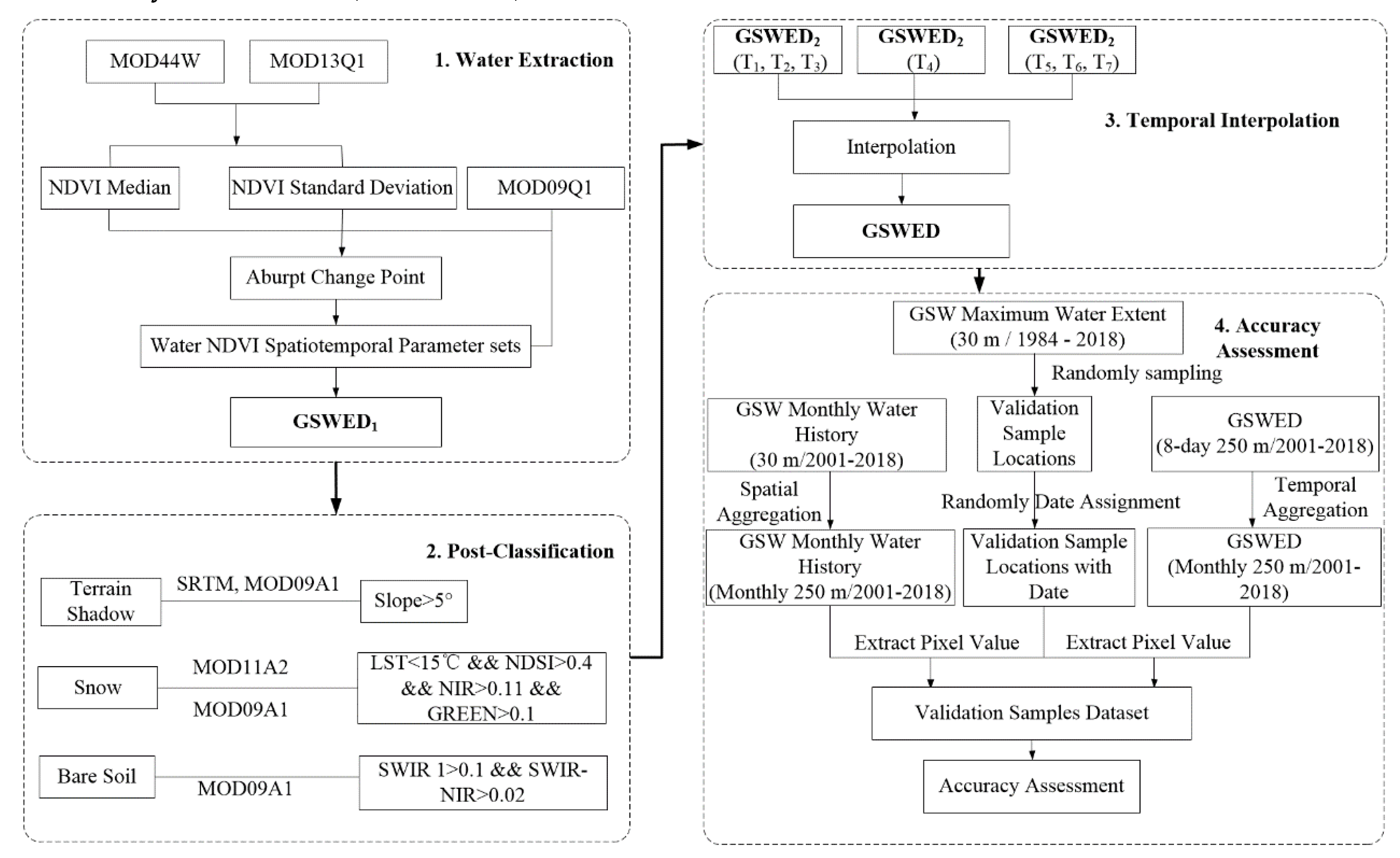
Figure 2.
Time series curves of the normalized difference vegetation index across different years for Balkhash Lake, Kazakhstan (a) and Xingkai Lake, China (b).
Figure 2.
Time series curves of the normalized difference vegetation index across different years for Balkhash Lake, Kazakhstan (a) and Xingkai Lake, China (b).
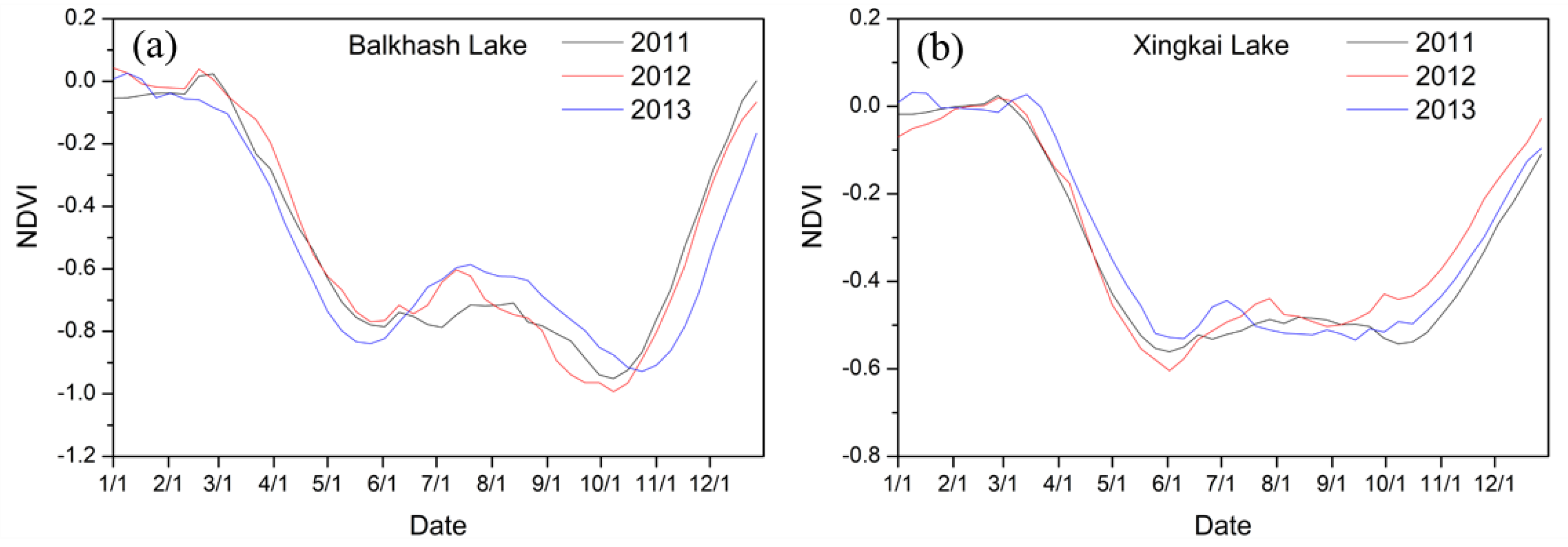
Figure 3.
Normalized difference vegetation index—water area difference (water area from NDVIi subtract water area from NDVIi-1, i = 1, 2, …, 21, NDVIi > NDVIi-1) curves and the optimal normalized difference vegetation index threshold for Qinghai Lake (a) and Poyang Lake (b).
Figure 3.
Normalized difference vegetation index—water area difference (water area from NDVIi subtract water area from NDVIi-1, i = 1, 2, …, 21, NDVIi > NDVIi-1) curves and the optimal normalized difference vegetation index threshold for Qinghai Lake (a) and Poyang Lake (b).
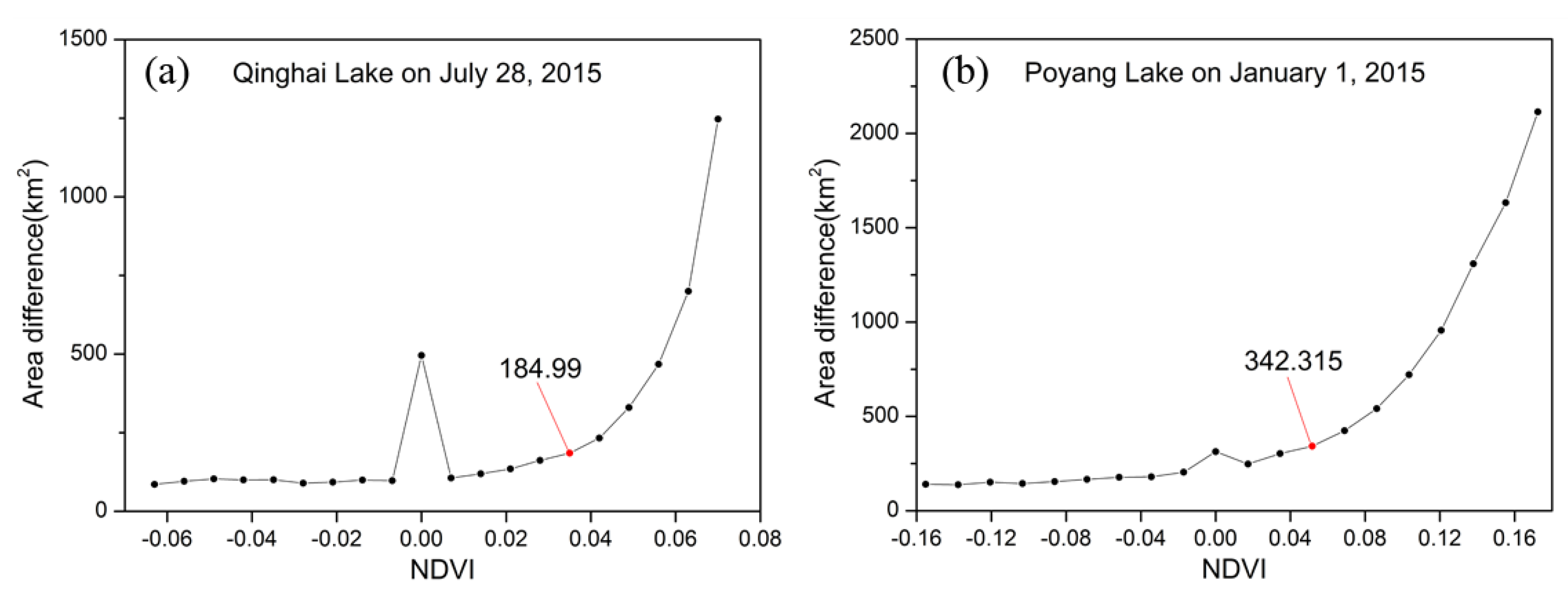
Figure 4.
Division of the global land (gray boxes were used for global surface water mapping), validation regions distribution (red boxes were used for accuracy validation) and number of validation sample points in every year (a) and month (b).
Figure 4.
Division of the global land (gray boxes were used for global surface water mapping), validation regions distribution (red boxes were used for accuracy validation) and number of validation sample points in every year (a) and month (b).
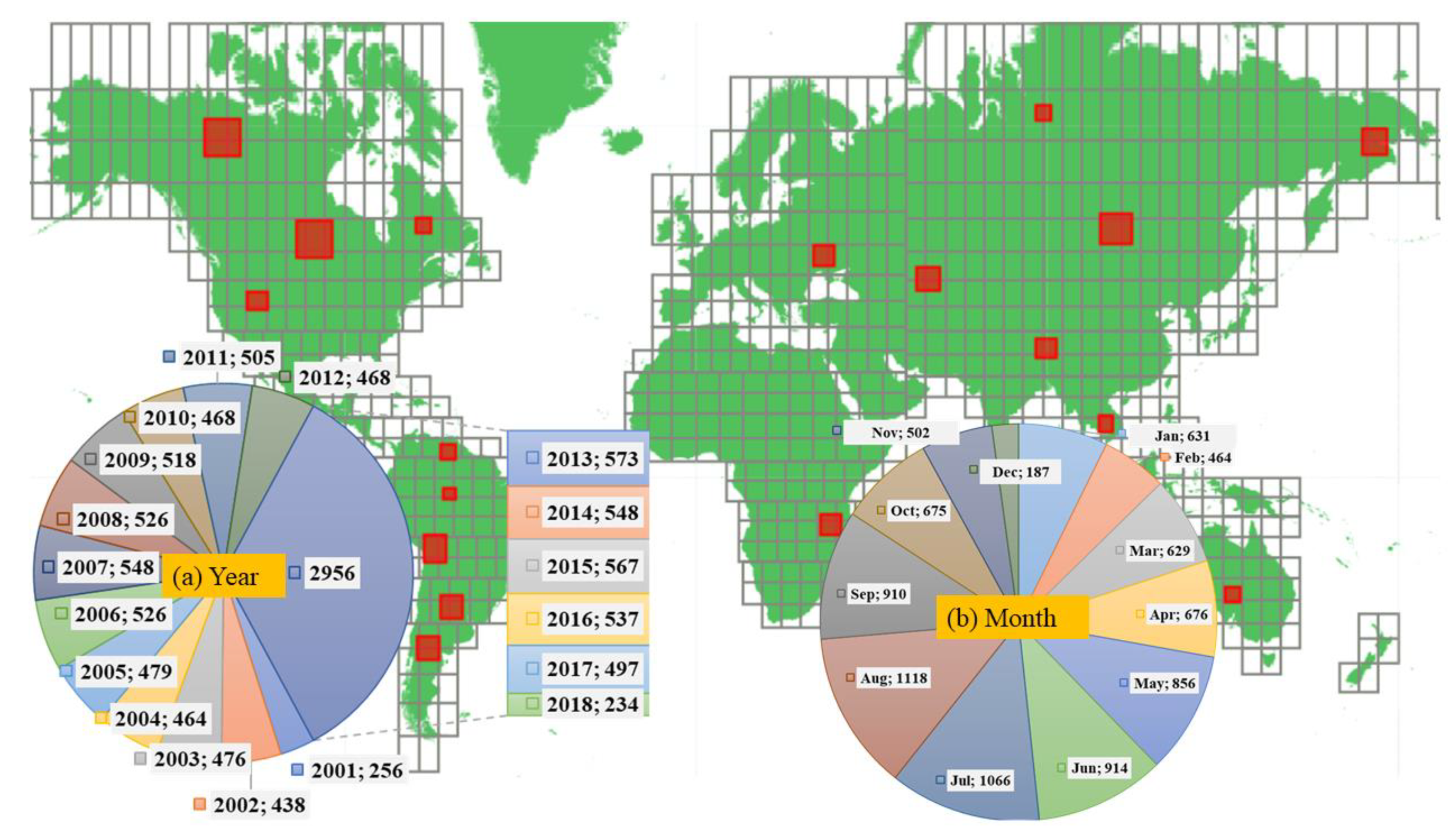
Figure 5.
Validation of global surface water extent dataset in 2015 in Qinghai Lake (a), Selin Co Lake (b), Utah Lake (c), and Dead Sea (d) using Landsat 8 OLI images.
Figure 5.
Validation of global surface water extent dataset in 2015 in Qinghai Lake (a), Selin Co Lake (b), Utah Lake (c), and Dead Sea (d) using Landsat 8 OLI images.
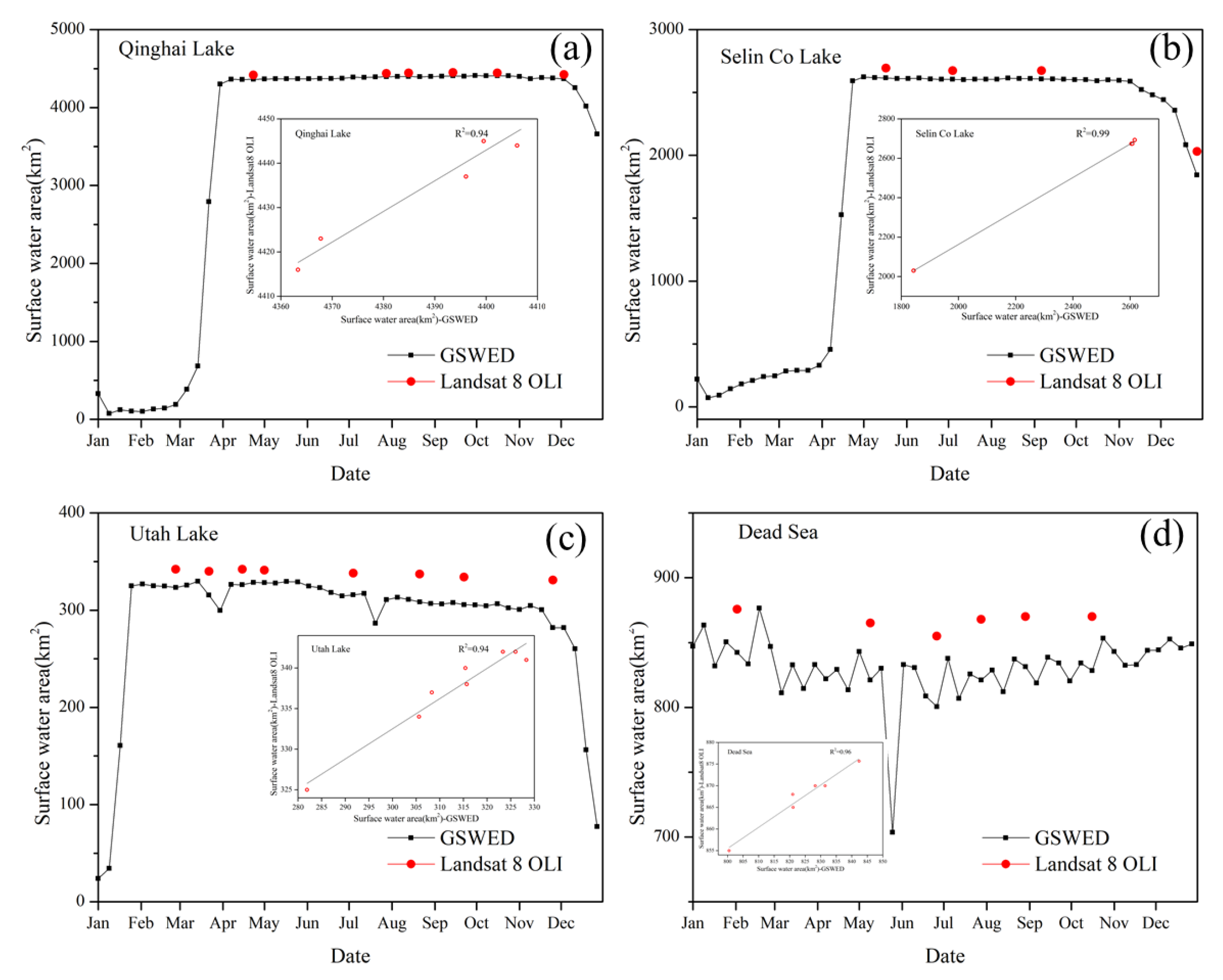
Figure 6.
Latitudinal (a) and longitudinal (b) maximum area comparison for global surface water extent dataset and MOD44W between 2000 and 2015.
Figure 6.
Latitudinal (a) and longitudinal (b) maximum area comparison for global surface water extent dataset and MOD44W between 2000 and 2015.

Figure 7.
Changes in global water area from the year 2000 to 2018.
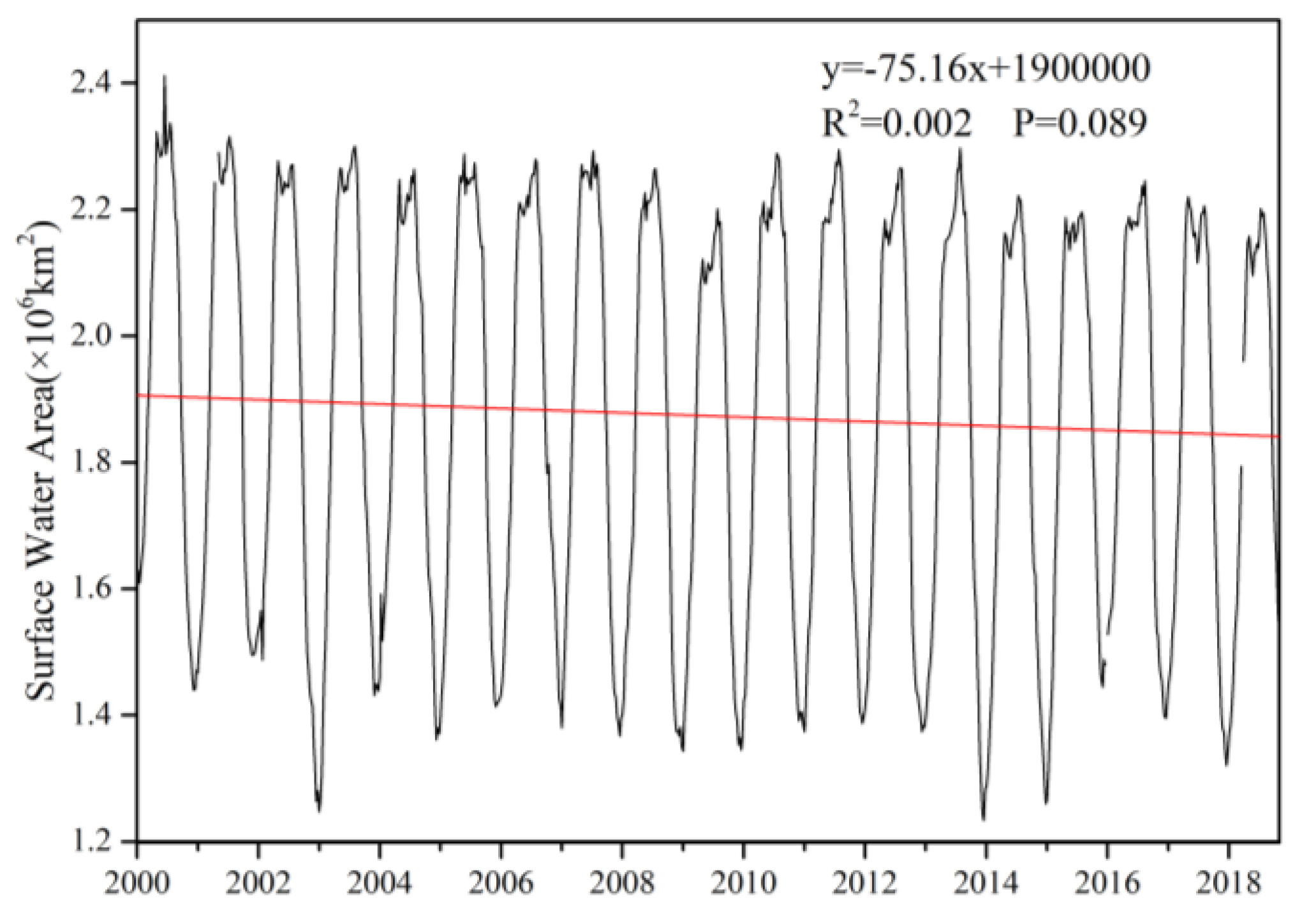
Figure 8.
Water occurrence of Selin Co Lake (a1), Urmia Lake (a2), and the Aral Sea (a3); water areal changes of Selin Co Lake (b1), Urmia Lake (b2), and the Aral Sea (b3) from 2000 to 2018.
Figure 8.
Water occurrence of Selin Co Lake (a1), Urmia Lake (a2), and the Aral Sea (a3); water areal changes of Selin Co Lake (b1), Urmia Lake (b2), and the Aral Sea (b3) from 2000 to 2018.

Figure 9.
(a) Water occurrence and (b) water area changes of Chiquita Lake from 2000 to 2018; (c) monthly average water level of Chiquita Lake [50].
Figure 9.
(a) Water occurrence and (b) water area changes of Chiquita Lake from 2000 to 2018; (c) monthly average water level of Chiquita Lake [50].
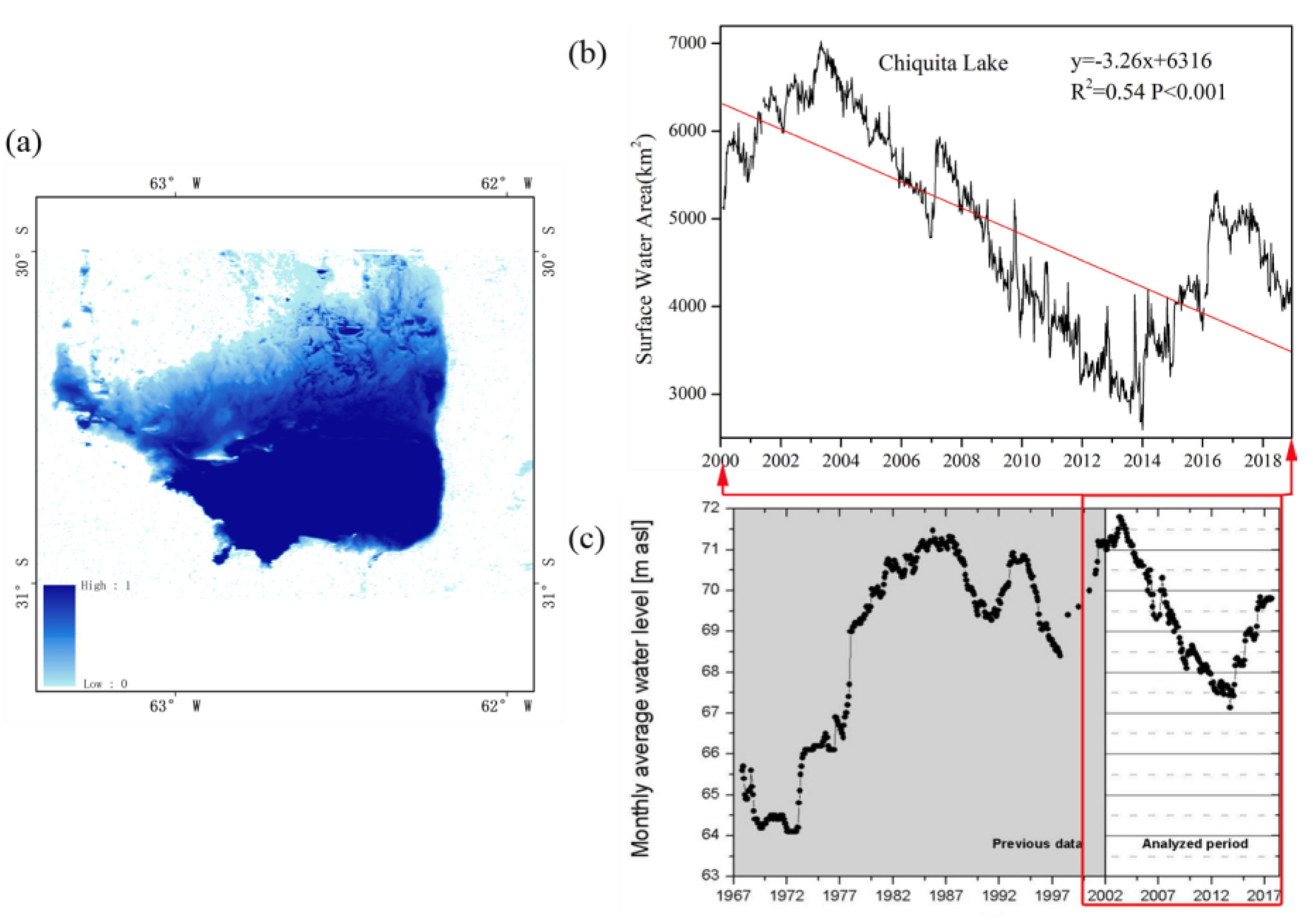
Figure 10.
(a) Areal changes of Dongting Lake water area from 2011 to 2013; (b) water level of Dongting Lake from 2011 to 2013 [51].
Figure 10.
(a) Areal changes of Dongting Lake water area from 2011 to 2013; (b) water level of Dongting Lake from 2011 to 2013 [51].
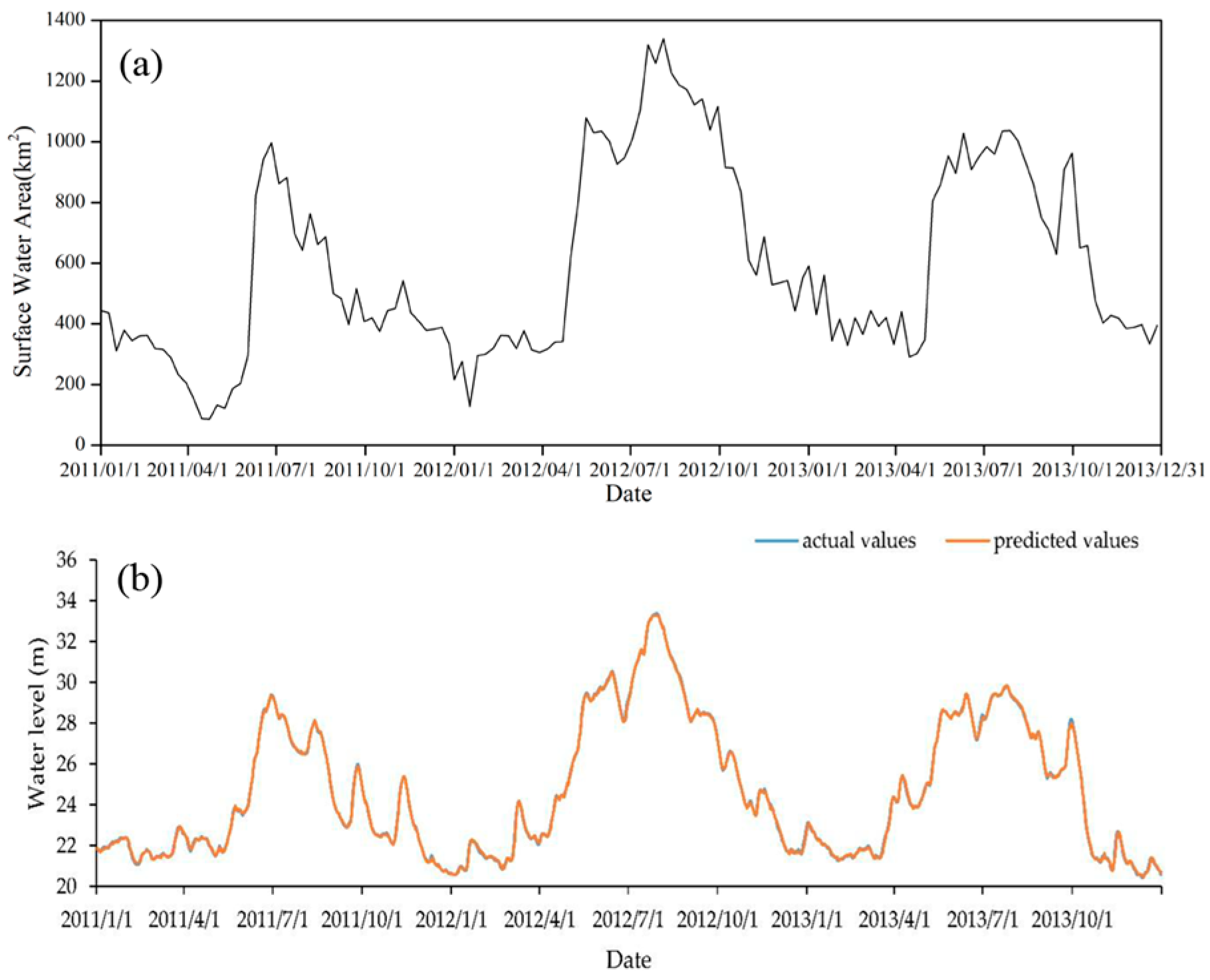
Figure 11.
(a) Changes in surface water area of global surface water [25] and global surface water extent dataset in Songhuajiang basin in 2013 and in Poyang Lake in 2015, China; (b) surface water distribution of Ji et al. [26] and our dataset in Poyang Lake on June 26, 2015.
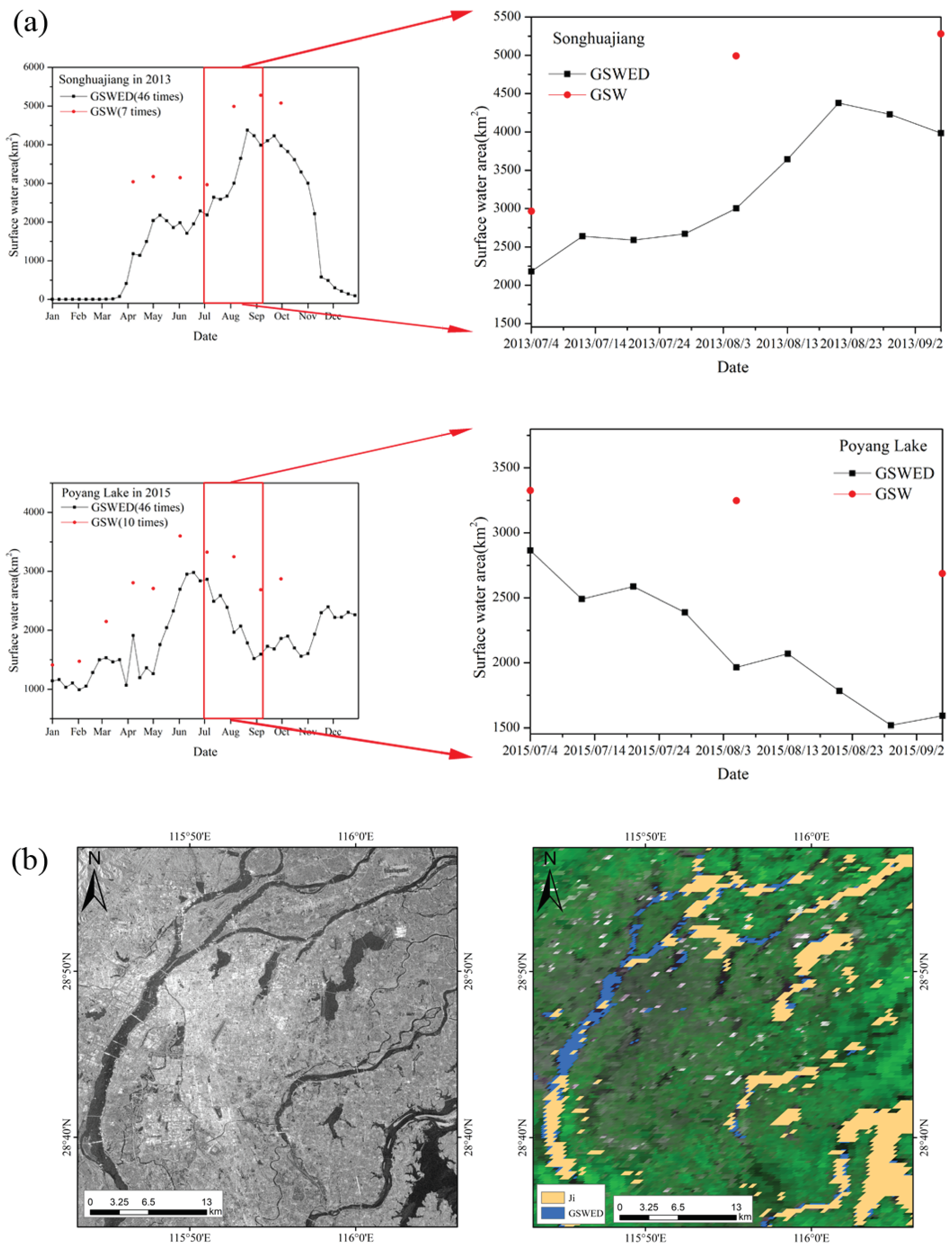
Figure 12.
(a) Water extracted by short wave infrared band [26] and the global surface water extent dataset in Poyang Lake on 26 June 2015 and (b) water extracted by the modified normalized difference water index and global surface water extent dataset in Winnipeg Lake in North America on 28 July 2015.
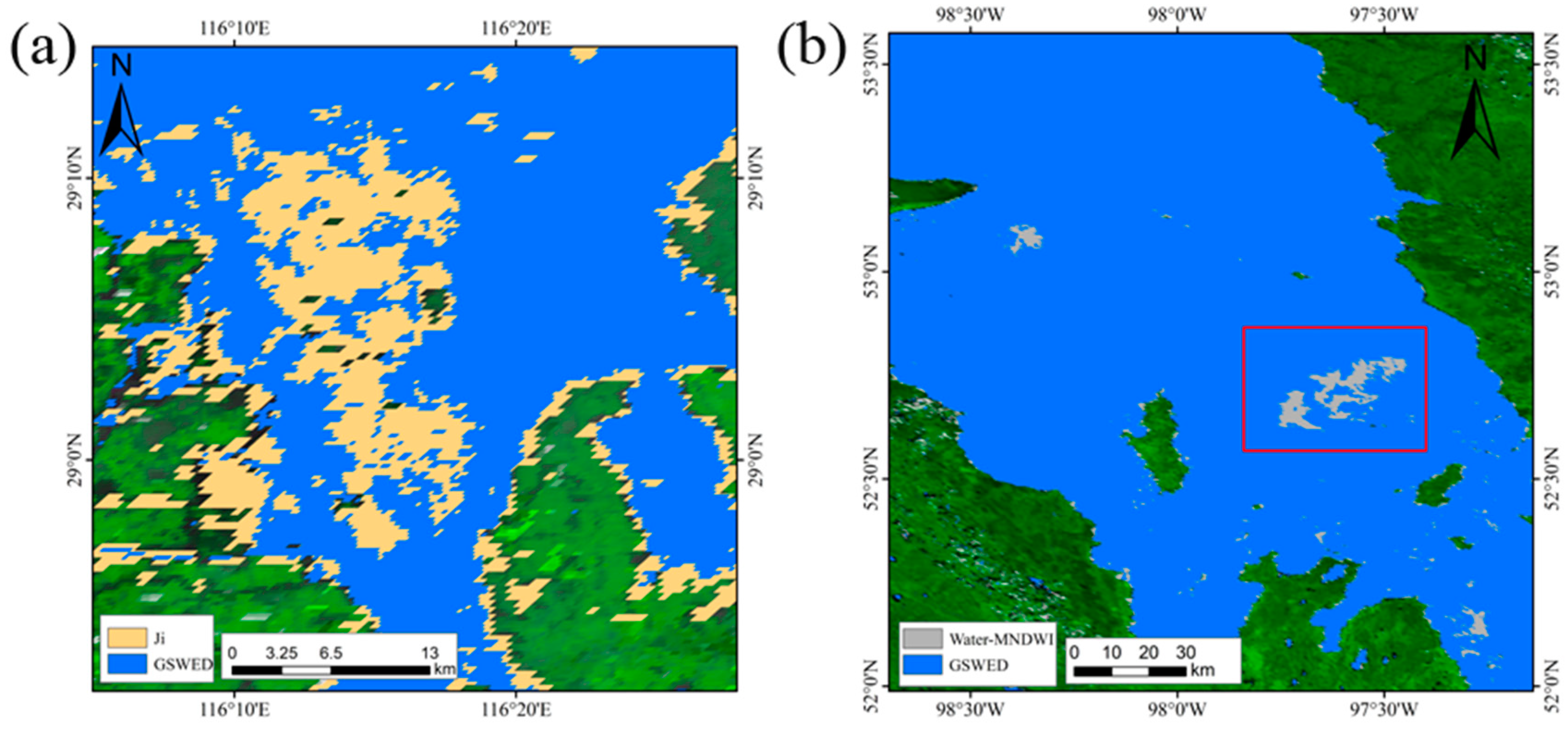
Figure 13.
Changes in surface water area according to Ji [26], global surface water [25] and the global surface water extent dataset in Dongting Lake (a), Chiquita Lake (b), Aral Sea (c), and the Dead Sea (d) in 2015.
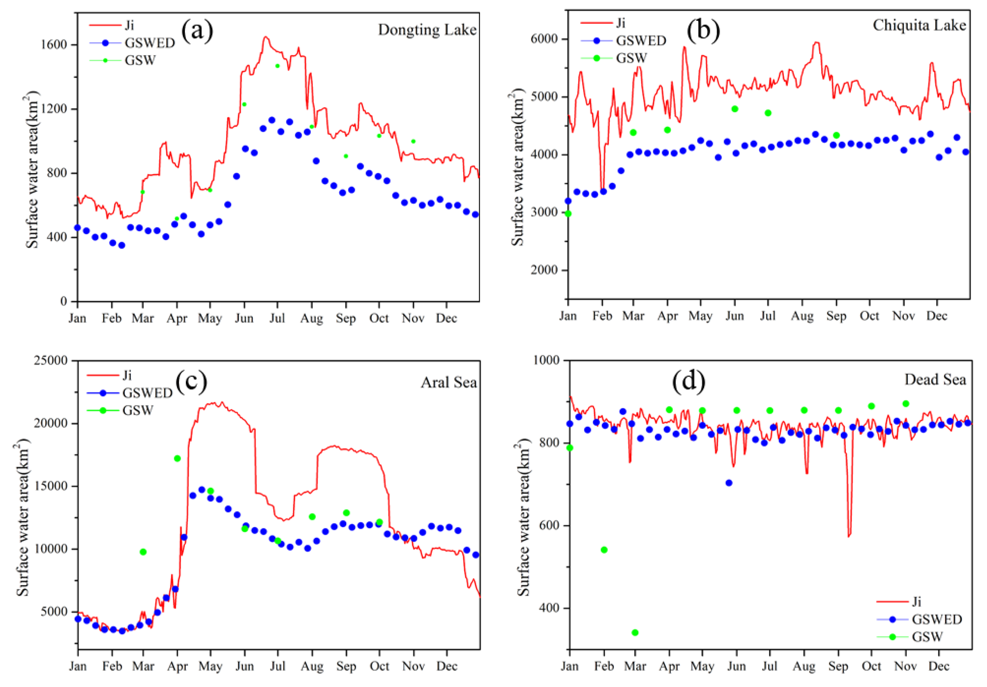
Figure 14.
Comparison of water normalized difference vegetation index thresholds between the OTSU threshold and manual threshold, taking Poyang Lake (a) and Xingkai Lake (b) as examples.
Figure 14.
Comparison of water normalized difference vegetation index thresholds between the OTSU threshold and manual threshold, taking Poyang Lake (a) and Xingkai Lake (b) as examples.

© 2020 by the authors. Licensee MDPI, Basel, Switzerland. This article is an open access article distributed under the terms and conditions of the Creative Commons Attribution (CC BY) license (http://creativecommons.org/licenses/by/4.0/).
Share and Cite
MDPI and ACS Style
Han, Q.; Niu, Z. Construction of the Long-Term Global Surface Water Extent Dataset Based on Water-NDVI Spatio-Temporal Parameter Set. Remote Sens. 2020, 12, 2675. https://doi.org/10.3390/rs12172675
AMA Style
Han Q, Niu Z. Construction of the Long-Term Global Surface Water Extent Dataset Based on Water-NDVI Spatio-Temporal Parameter Set. Remote Sensing. 2020; 12(17):2675. https://doi.org/10.3390/rs12172675
Chicago/Turabian StyleHan, Qianqian, and Zhenguo Niu. 2020. "Construction of the Long-Term Global Surface Water Extent Dataset Based on Water-NDVI Spatio-Temporal Parameter Set" Remote Sensing 12, no. 17: 2675. https://doi.org/10.3390/rs12172675
Note that from the first issue of 2016, this journal uses article numbers instead of page numbers. See further details here.