A Machine Learning Approach to Detecting Pine Wilt Disease Using Airborne Spectral Imagery
by
 and
and
Marian-Daniel Iordache
1,*, 
Vasco Mantas
2,
Elsa Baltazar
2,
Klaas Pauly
1 and
Nicolas Lewyckyj
1 1
Flemish Institute for Technological Research, Center for Remote Sensing and Earth Observation Processes (VITO-TAP), Boeretang 200, B-2400 MOL, Belgium
2
Department of Earth Sciences, University of Coimbra, 3004-531 Coimbra, Portugal
*
Author to whom correspondence should be addressed.
Remote Sens. 2020, 12(14), 2280; https://doi.org/10.3390/rs12142280
Submission received: 22 May 2020
/
Revised: 4 July 2020
/
Accepted: 8 July 2020
/
Published: 15 July 2020
(This article belongs to the Special Issue Forest Degradation Monitoring)
Abstract
:Pine Wilt Disease is one of the most destructive pests affecting coniferous forests. After being infected by the harmful Bursaphelenchus xylophilus nematode, most trees die within one year. The complex spreading pattern of the disease and the tedious hard labor process of diagnosis involving field wood sampling followed by laboratory analysis call for alternative methods to detect and manage the infected areas. Remote sensing comes naturally into play owing to the possibility of covering relatively large areas and the ability to discriminate healthy from sick trees based on spectral characteristics. This paper presents the development of machine learning classification algorithms for the detection of Pine Wilt Disease in Pinus pinaster, performed in the framework of the European Commission’s Horizon 2020 project “Operational Forest Monitoring using Copernicus and UAV Hyperspectral Data” (FOCUS) in two provinces of central Portugal. Five flight campaigns have been carried out in two consecutive years in order to capture a multitemporal variation of disease distribution. Classification algorithms based on a Random Forest approach were separately designed for the acquired very-high-resolution multispectral and hyperspectral data, respectively. Both algorithms achieved overall accuracies higher than 0.91 in test data. Furthermore, our study shows that the early detection of decaying trees is feasible, even before symptoms are visible in the field.
1. Introduction
Biotic agents are a significant threat to the sustainability of forest ecosystems worldwide, all the more so as global trade facilitates their spread beyond original ranges. Pine Wilt Disease (PWD), caused by the pinewood nematode (Bursaphelenchus xylophilus) offers such an example. Native to North America, it spread first to Japan in 1905 [1] and later to other Asian countries including China (1982) and Korea (1988).
Unlike what is observed in North America, where host trees are relatively tolerant, widespread damage to trees in the affected countries was reported. Despite intense efforts made by the Japanese government to limit the economic impact of the disease, it is estimated that Japanese forests lost more than 46 million cubic meters of trees over the last 50 years [2].
In 1999, PWD was first detected in Europe [3], triggering a complex and ongoing containment effort, which slowed but did not stop the expansion of PWD in Portugal. Authors in [4] concluded that temperature plays a crucial role in the development of the PWD: the mean air temperatures should be higher than 20 °C for long periods in order to observe a strong effect of the disease throughout the forest. Thus, PWD originates from the presence and interaction of the harmful nematode, beetle vector and favorable environmental conditions. Given the continuous increase of average temperatures around the Earth in the recent years, it can be deduced that more and more areas on Earth are prone to become welcoming ranges for PWD, thus the threat posed by the disease is steadily increasing. In [5], it is shown that the Mediterranean areas might be an especially vulnerable region to global climate change, while in [6] the authors estimate that the mean temperature increase in Portugal occurred at a rate of 0.52 °C decade−1 between 1976 and 2006. This trend in increasing temperatures continues to date, as revealed by multisource observations such as the ERA5 dataset freely accessible through the European Union’s Copernicus Climate Change Service (C3S) Climate Data Store (CDS) [7]. For example, the number of air temperature anomalies relative to the 1980–2010 average plotted in Figure 1 shows that hot temperature anomalies (in red) are also increasingly dominant over cold temperature anomalies (blue) in Portugal in the last decade.
In Portugal, the favorable conditions for the PWD are thus easily met: the climate is relatively warm across the whole year, plenty of Monochamus galloprovincialis beetles (insect vector for PWD) roam over large pine forests and, moreover, the country is strongly connected with the worldwide maritime trade routes via the commercial ports on the Atlantic coast. The disease was first confirmed in the Setúbal Peninsula in 1999 [3], where the nematode was presumably introduced by internationally transported goods, which triggered an alarm not only in Portugal, but at European level.
Despite quarantine measures established around the first affected areas, the disease could not be stopped from spreading in other parts of the country. Human activities are an important factor among those stimulating this spread. As a consequence of infected wood transportation, infected trees were also found in Spain in 2008 [8,9].
Since the B. xylophilus nematode, carried by the Monochamous beetle, was identified as the cause of PWD, consistent research was carried to better describe the dispersal patterns of the disease, the nematode itself (e.g., taxonomy, genetic structure, embryology and morphobiometry of the nematode), the transmission vector (e.g., biology, ecology, life cycle and development stages of the beetle), the nematode–vector–host interactions, the mechanisms of wilting, triggered by the disease, the management of the disease (e.g., breeding resistant trees, control of insect populations, chemical methods, biological methods), among others. For a detailed coverage of these topics, the reader is referred to [10,11] and the references therein.
One critical goal in the management of the PWD is to identify and remove affected trees from site before the disease spreads to other (healthy) trees by the vector insect. Trees with visible symptoms can be identified by a human observer due to specific symptoms such as discoloration and defoliation. However, the symptoms of the disease usually appear first on top branches, which are harder to observe from the ground. The presence of the nematode can be confirmed by laboratory analysis after collecting woody samples from trees. In practice, it is impossible to collect samples from all trees, which leads to the necessity of identifying infected ones from a distance over relatively large areas. Therefore, remote sensing comes naturally into play as a viable alternative to complete this important management task.
Coniferous trees infected with B. xylophilus generally display a set of nonspecific symptoms, which are caused by the disruption of the host’s vascular system. The symptoms include discoloration (yellow to brown) and wilting of needles as well as a reduction of resin exudation, onsetting usually from late summer to late autumn [11]. The changes observed in key physiologic variables in infected trees, including the significant drop in the concentration of pigments, translate into a rapid change of the reflective spectrum in the visible and near infrared range. The nonspecific set of symptoms, as observed with the naked-eye, can be classified according to somewhat subjective discoloration or defoliation levels, as in [12]. Ideally, remote sensing sensors should be able to provide objective and reproducible decline metrics. Furthermore, the absence of PWD-specific symptoms impedes a field confirmation of infection by this biotic agent. Instead, laboratorial analyses are required, adding to the costs and complexity of surveying actions.
Various approaches devoted to the identification and management of the PWD are available in the literature. In [13], the authors classify the dispersal patterns of the PWD into four categories: jumping, unidirectional direction, multidirectional extension and static (no dispersal), while a correlation between the human population density and the annual dispersal distance is revealed. The authors in [14] also note that approximately 80% of the damaged trees detected in one year are found within a distance of 60 m from dead trees in the previous year. However, the traveling distances of the insect vector can be in the order of hundreds or even thousands of meters. Several works also investigate the PWD detection from a remote sensing perspective, via spectral measurements, although their number is still limited. A ground-based hyperspectral camera was employed in [15] to detect PWD symptoms from the spectral signatures of the observed pixels. After analyzing four spectral indices, it is reported that the measured reflectance at the wavelength of 668 nm is the most useful indicator in separating the diseased trees from the healthy trees. In [16], the authors note that the spectral evolution of the diseased trees from a temporal point of view is reflected by important changes of the measured reflectance in the red and SWIR (short-wave infrared) spectral regions. The ability of multispectral cameras to detect stress symptoms in coniferous trees is investigated in [17], where the authors induce an artificial stress to several trees by inoculating them with herbicide. Although this approach simulates a generic disease outbreak and does not specifically treat the PWD problem, it proves that the stressed trees can be identified by spectral approaches, particularly in the red-edge region of the spectrum. An experiment involving controlled PWD inoculation in healthy trees is presented in [18]. Subsequently, a field spectrometer was used to measure the spectral characteristics of the monitored trees along a pre-defined period of time and 11 discriminative indices were computed for all measured points, from which the most discriminative ones are highlighted. The authors also show that the evolution of the disease over time is clearly noticeable in the spectral region 550–670 nm of the observed spectra. In [19], the ability of a large set of spectral indices to distinguish between healthy and decaying pine trees was tested for aerial and satellite imagery, in a buffer area established by the Spanish authorities in the region of Extremadura, near the border with Portugal. Most of those indices were found to be informative due to the statistically significant differences found between the sets of healthy and infected trees. The thermal imagery can also be useful in PWD detection, but it should be used during hot summer days in order to be relevant, as previously observed for other tree species affected by pests (e.g., date palm red weevil [20,21]). The authors identify five highly informative wavelengths among the considered ones, propose the use of high spatial resolution imagery for the analysis at tree level, jointly with recommendations related to minimum data quality and identify strategies for the mitigation of high costs in an operational setup, among others, all these contributions transforming their work in one of the most valuable manuscripts in the area of PWD monitoring.
Our work combines the individual advantages of previous works in various aspects, jointly with an extension of the tested sets of indices and new classification algorithms. Understanding the distribution of PWD using practical methods capable of depicting the situation in multiple scales and even in remote locations, is critical to develop innovative distribution models to assist the implementation of control strategies. Similarly to [17,18,19], the goal of our approach is to detect infected trees based on remote sensing approaches. We propose the use of two distinct (multi/hyperspectral) cameras in a temporal experiment covering two consecutive years (2018 and 2019) in order to investigate the possibility of detecting infected trees at a very early stage of the disease and to capture the temporal evolution of the affected areas. The set of investigated spectral indices is enlarged in comparison to the ones from previous studies and we propose new per-pixel classification algorithms, based on Random Forest approaches, for the detection of infected trees.
In summary, our work explores a variety of scientific directions in order to respond to two fundamental questions: (i) How accurate are the PWD maps derived from very-high-resolution spectral data acquired from remotely piloted aircraft systems (RPAS)? (ii) Is the early detection of PWD feasible? In order to find answers to these questions, our study brought together several strengths in PWD research that can be summarized as follows: (i) the selected test areas were located in central Portugal, a region where the presence of the PWD was confirmed; (ii) one multispectral camera and one hyperspectral camera, jointly with an RGB camera, were deployed in the area, carried by RPAS; (iii) five data acquisition campaigns were carried out in 2018 and 2019; (iv) the informative metrics were selected from larger sets of spectral indices than in any previous study; (v) classification algorithms were separately built for the multispectral and hyperspectral data, respectively; (vi) a new set of informative wavelengths was derived; (vii) the feasibility of early detection was investigated; and (viii) the potential to capture the temporal evolution of the disease by spectral cameras mounted on RPAS was analyzed.
2. Materials and Methods
2.1. Data Preparation
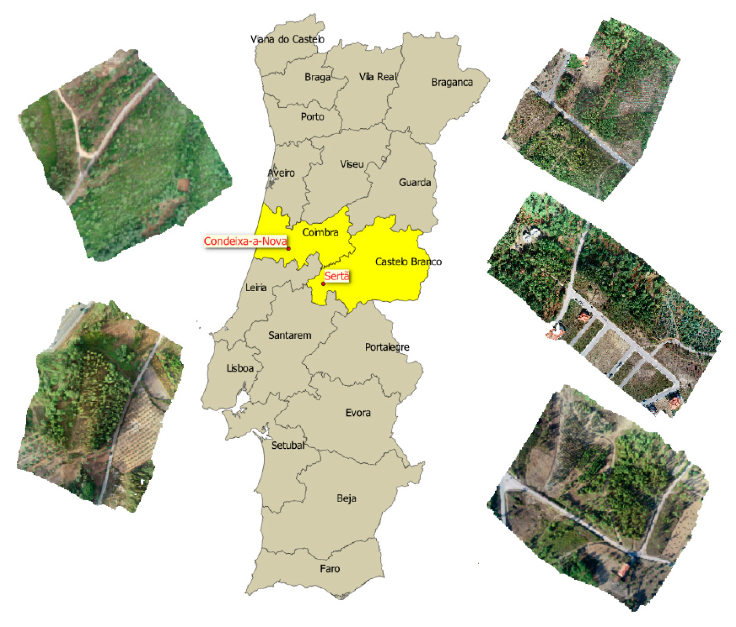
Five test areas, located in central Portugal and accounting for a total area of approximately 23 ha, were chosen for the study, as illustrated in Figure 2: two sites near the town of Condeixa-a-Nova (Coimbra district) and three sites near the town of Sertã (Castelo Branco district). PWD is confirmed to be present in these areas [11].
Five flight campaigns were organized along two years: June 2018, October 2018, June 2019, September 2019 and October 2019. After the first campaign, one site near Condeixa-a-Nova (lower left RGB image in Figure 2) was discarded as it was devastated on October 13, 2019, by post-tropical storm Leslie, the strongest cyclone to hit the Iberian Peninsula since 1842.
The measurements were scheduled in early summer and mid-autumn due to the temporal flight pattern of Monochamus galloprovincialis. The flight season of the insect starts in May each year and lasts until late summer or early autumn, with some interannual variability [22]. Thus, the moments of the flights correspond to the early infection stage (June), when PWD symptoms in the field are extremely scarce apart from dead trees infected the previous year, and fully symptomatic infection, where symptoms at different stages can be observed (October). The flight campaign in September 2019 was interposed in order to check the ability of classification methods to capture variations in the field on relatively short periods of time (i.e., one month).
Two spectral cameras with distinct characteristics were used to acquire imagery over the test sites. Both cameras were mounted on RPAS operated by certified pilots from the Flemish Institute for Technological Research (VITO). During all flights, spectral targets (grey and green colors) were placed in the field of view of the sensors for calibration purposes. Concurrent with the data acquisition, spectral measurements were performed in the test areas using ASD FieldSpec4 spectrometers (https://www.malvernpanalytical.com/en/products/product-range/asd-range) to allow for subsequent data quality assessment. Geometric targets were also deployed in the field and their positions, measured with high-accuracy GPS devices, were used in the preprocessing of the data as ground control points for improved georeferencing. The raw data, jointly with all auxiliary data, were processed by VITO experts up to reflectance products which constitute the input for training in the classification algorithms.
The first system used in the experiments is the multispectral camera MicaSense Red-Edge M (https://www.micasense.com/), benefitting from five spectral bands centered at 475 nm (blue), 560 nm (green), 668 nm (red), 717 nm (red-edge) and 840 nm (near-infrared) and having bandwidths (FWHM) of 20 nm, 20 nm, 10 nm, 10 nm, 40 nm, respectively. The MicaSense wavelengths are listed among the most informative ones for PWD detection in [15,19]. Four of its spectral bands (bands 1, 2, 3 and 5) largely overlap with Sentinel-2 bands (bands 2, 3, 4 and 8), while the fourth band partially overlaps with the fifth band of Sentinel-2, meaning that a large number of spectral indices can be computed for MicaSense in a way which is similar to Sentinel-2. The MicaSense RedEdge was mounted on a DJI Phantom 4 Pro quadcopter alongside its integrated 20 MP RGB camera.
The second system used for data acquisition is the MicroHyperSpec A-series VNIR–Visible and Near Infra-Red (https://www.headwallphotonics.com/hyperspectral-sensors) hyperspectral pushbroom scanner. This camera samples the spectral region 380–1000 nm in 324 spectral bands with a spectral resolution of 1.9 nm and FWHM of 5.8 nm. The large number of bands allows for the calculus of more spectral indices than in the case of multispectral cameras. The MicroHyperSpec was mounted on an Aerialtronics ATX-8 Zenith coaxial octocopter platform.
Flights were planned at a fixed flying height on average 45 m above the canopy level at the highest terrain point in each area of interest (i.e., around 80 m above the highest ground level), with 85% overlap set in the forward and lateral direction for RGB and multispectral imagery and 30% lateral overlap between hyperspectral scan lines. In general, five ground control points markers (GCPs) were installed in each area of interest and measured with Real Time Kinematic (RTK) Global Navigation Satellite Systems (GNSS) in the Portuguese network of continuously operating reference stations Rede Nacional de Estações Permanentes GNSS-ReNEP (2–3 cm accuracy). The maximum number of GCPs that could be installed or used was ultimately dictated by the dense forest environment of the areas of interest. RGB and multispectral imagery was processed separately through a structure from motion (SfM) photogrammetry workflow in the commercial software Agisoft MetaShape 1.5.x. This workflow consists of tie-point extraction and matching (alignment), geometric camera calibration and refinement of the georeferencing based on the ground control points (optimization), reflectance calibration, dense point cloud generation, dense point cloud classification (into ground, above-ground and noise classes), raster digital surface model (DSM) generation based on the ground and above-ground point classes, raster digital terrain model (DTM) generation based on the ground points only, and orthomosaic generation based on the DTM. For hyperspectral imagery, the geometric correction is performed using VITO’s own developed C++ module and is based on direct georeferencing. Input data from the sensor’s Applanix APX-15 GNSS/INS, the sensor geometric model, boresight correction data and elevation data are further used during the geometric correction process. Orthomosaicing was then done per flight line based on the photogrammetrically derived DTMs. The photogrammetric processing resulted in georeferenced reflectance cubes for both data types: ENVI files (pairs of .img and .hdr files) for the hyperspectral data having a spatial resolution of 10 cm, and GeoTIFF (.tif) files for the multispectral data and RGB with a spatial resolution of 5 cm. RGB mosaics in GeoTIFF format were also created from data acquired by the RGB camera at a resolution of 2 cm. All imagery types were finally projected to Universal Transverse Mercator (UTM) coordinates.
Intensive monitoring of the five sites was performed along the two experimental years. Ground teams from University of Coimbra identified and monitored more than 120 trees. These trees were identified in the RGB imagery and used as the basis for the training stage of the classification algorithm. Figure 3 shows the distribution of training points in one site from Sertã.
During the monthly surveys, infected trees were mapped, when still at stage II or III of decline, as defined in [22]. A subset of these trees was selected for laboratorial analyses using the protocol described in [19]. If PWN was detected in the analysis, the tree was assigned to the class “infected”. Trees in close proximity to infected (spatial and temporal) and displaying similar symptoms but not tested were classified as “suspicious”. Trees showing no symptoms (green) were classified as “healthy”. The solution is based on a compromise between sampling effort and representativity.
Each of the training points was assigned to one of the following classes: “infected”—trees confirmed to be affected by the PWD by laboratory analysis; “suspicious”—trees showing symptoms of the disease at different stages, but not tested in the laboratory for PWD; “healthy”—(green) trees showing no signs of the disease. The trees in the “infected” class were in level II or III of canopy degradation, as aforementioned, due to the fact that lab analysis is usually performed on trees that can be clearly identified as symptomatic, in the absence of other information. However, all the trees used for training and belonging to the “suspicious” class displayed compatible symptoms and no tree recovered during the experiment—all of them died after different periods of time. The combination of symptoms, timing and sampling strategy suggests a very high likelihood of the presence of the disease across a high proportion of the “suspicious” trees. Thus, confusions between the “infected” and “suspicious” classes can be tolerated to certain extent, but the healthy trees should be clearly separated from the other classes.
Once the set of training points was defined, each tree was identified in the multi-/hyperspectral imagery and region growing algorithms were employed to extract the respective tree crown. The corresponding spectra were then extracted from the imagery and stored in the corresponding training database. This way, two distinct training databases were obtained, corresponding to multi- and hyperspectral data, respectively. Figure 4 shows examples of delimited crowns and extracted spectral signatures. Note that, even for one single crown, large heterogeneity of signatures is easily noticeable with respect to shape and amplitude.
Table 1 shows an overview of the number of trees (per class) and the corresponding number of data points extracted from available imagery. Note that the number of infected trees is low in comparison to the number of suspicious and healthy trees, as only three trees were confirmed to be infected by PWD following the laboratory analysis, at the time of the training data definition (October 2018). However, considering the sampling strategy adopted and the overwhelming rate of positive cases in analyzed trees, it is likely that suspicious cases were equally infected.
2.2. Selection of Discriminative Metrics and Wavelengths
Starting from the reflectance spectra of the training pixels, comprehensive sets of spectral indices (also named “metrics” in the following) were defined. These metrics were found in the literature (see, e.g., [19] and the references therein) and in databases of spectral indices available online (see, e.g., https://www.indexdatabase.de/). At the end, 25 metrics were built for the multispectral data, and 74 metrics for the hyperspectral data. These metrics are intended to capture the different features of the healthy, suspicious and infected trees. However, it is well known that a multitude of metrics used in classification does not always guarantee a better performance. Some metrics could lack power of discrimination, while others could be highly correlated. Further, the use of a large number of parameters implies higher computational burden. Thus, filtering of these metrics is needed before employing them in a classification scheme.
Two distinct approaches were used for metrics filtering. In multispectral data, an iterative classification scheme selects metrics from the list based on their correlation with other metrics, intraclass variation and interclass distances. Specifically, after the values of each metric are normalized using a peak-to-peak approach, the selection is performed as follows. For every metric, we first define a discriminative parameter R, calculated as the ratio between the interclass distance and the intra-class variation. The interclass distance is computed as the average distance between the centroids of the considered metric in all classes, while the intraclass variation is computed as the average of the standard deviations of the considered metric in all classes. Second, the Pearson correlations are computed for all possible pairs of metrics. Third, a threshold T is chosen to define the maximum allowed correlation between any two metrics. Then, for each pair of metrics with correlation larger than T, the metric with lower R is removed from the list of metrics. The idea behind this selection is that the centroids of one metric, computed per class, should be as far as possible from each other, while the spread of the metric should be as low as possible in each class. Thus, R should be as high as possible to promote separability of the classes. The result of this iterative selection is a set of metrics in which the maximum correlation between any pair of metrics is lower than T. After assessing the performance of various sets of metrics in terms of classification performance, the maximum allowed correlation was set to T = 0.95 in our experiments. In hyperspectral data, the selection method was borrowed from the classification methodology of the PROBA-V land cover product [23] and it selects metrics based on their discriminative power in a classification scenario. At the end, 13 indices were kept for the training stage for both multispectral and hyperspectral data.
The metrics filtering performed in hyperspectral data is not only intended to reduce the number of metrics used in classification, but also to derive a set of informative wavelengths that could be used in the design of a multispectral camera tailored to the specific application of PWD. These wavelengths are the ones used to compute the selected hyperspectral metrics.
2.3. Classification Algorithms and Postprocessing Strategies
Random Forest classification algorithms [24] were separately developed for the multi- and hyperspectral data.
Due to the low number of infected trees available for training (shown in Table 1), the sets of points corresponding to the different classes are strongly unbalanced w.r.t. sizes for both multi- and hyperspectral datasets. This characteristic could lead to the so-called “accuracy paradox”, i.e., biased classification output when the overall accuracy is used as the main performance discriminator. In order to avoid such issues, we have built balanced training sets by randomly selecting spectra corresponding to the three classes. The number of these spectra is 10% lower than the total number of points from the “infected” class. Thus, for the multispectral data, a number of 2055 points per class were kept to define the input dataset, while, for the hyperspectral data, 2344 points per class were selected for the same purpose. By following this approach, a drastic undersampling of the available training points for the healthy and suspicious classes was introduced. The algorithms were developed using the Random Forest Classifier meta estimator from the scikit-learn machine learning library [25] in Python 3.6.8 [26], with a random split of 70%/30% of data points for training and testing, respectively. Both schemes use the default parameterization, except for an increased number of trees (500 instead of 100) and enforced balanced class weights.
To inspect the accuracy of the classification algorithms, we use the following accuracy metrics:
Overall accuracy (OA): ratio between the number of correctly classified points and the total number of points;
Producer accuracy (PA): ratio between the number of correctly classified pixels from a class and the true number of points assigned to the same class;
User accuracy (UA): ratio between the number of correctly classified pixels from one class and the total number of points identified by the classifier as belonging to the same class.
Table 2 shows the confusion matrices, user accuracies, producer accuracies and overall accuracies for the two algorithms. In this table, note that OA exceeds 0.91 in both cases. Larger confusion can be observed between the infected and suspicious classes. In practice, this confusion is largely tolerated, as trees showing PWD symptoms are preferably removed from the field, even if no laboratory analysis is performed. In Portugal (and Europe in general), the removal of symptomatic trees is actually a legal obligation of the forest owners.
The accuracy metrics from Table 2 are graphically represented in Figure 5 by the Receiving Operator Characteristics (ROC) curves, per class, produced following the methodology in [25] and the implementation of the authors available online. The high performances of the classifiers are confirmed by the ROC curves. The “suspicious” class is in both cases prone to more confusion with the other classes. The “infected” class is spotted with high accuracy by both classifiers, due to its distinct spectral characteristics rooted in the class definition (i.e., trees in an advanced stage of degradation). Additional experiments, not reported here, have shown that this class can be discriminated with higher accuracy than the other two classes even under suboptimal training conditions (e.g., very low number of training samples and/or very low number of Random Forest trees), while the accuracy for the other two classes degrades under such conditions. As shown in Table 2 and Figure 5, the “suspicious” and “healthy” classes are also detected with high accuracy. Despite the fact that both training and testing pixels were randomly selected from data acquired in 2018, possible spatial correlation issues that could lead to the overestimation of the accuracy metrics are largely mitigated due to the following reasons: (i) as a consequence of the strong undersampling of the “healthy” and “suspicious” classes, the percentage of training points for these classes was extremely low (1–2%) in comparison to the number of available points extracted from the imagery, such that relatively large distances between training and testing points are enforced, even if they might be placed on the same crown; (ii) the data employed in this study are very high spatial resolution data (5/10 cm for multi-/hyperspectral data), thus the high heterogeneity of crown pixels illustrated in Figure 4 and induced by factors such as leaf density and orientation, light scattering and exposed branches, among others, is captured by the pixel spectra. In this type of data acquired from RPAS, significant spectral differences occur in terms of both shape and amplitude, e.g., differences larger than 100% in reflectance values, per band, are not uncommon even for spatial windows as small as 5 × 5 pixels, or 25 × 25 cm2 in multispectral data. All these factors contribute to mitigating potential autocorrelation issues. Furthermore, the classification maps obtained by the designed algorithms in data acquired in 2019 confirm that the classification schemes perform as expected in newly acquired imagery (see, e.g., Figure 14 in Section 3).
As the classification algorithms are trained exclusively on canopy spectra, pixels that do not belong to tree canopies could be assigned to any of the considered classes. This is not considered an algorithmic error, but it might result in maps that are difficult to interpret. In order to remove pixels falling outside tree canopies from the classification maps, various strategies are adopted, based on auxiliary data, spectral characteristics and spatial filtering.
First, a canopy height model (CHM) is computed by subtracting a digital terrain model from a surface terrain model used in the data georeferencing. The CHM thus measures the height of data pixels and thresholds can be used to remove points with low height. For example, if only ground pixels should be removed, all points having null CHM would be neglected.
Second, very dark pixels in the image usually correspond to shadowed pixels. Shadows generally occur below tree crowns, such that their removal does not impede the detection of infected trees, while ensuring a better visual appearance of the maps. The dark pixels are selected based on their intensity, i.e., pixels whose sum of band reflectance values falls below a predefined threshold are removed from the classification map.
Once the low pixels and the dark pixels are removed, noise can still affect the maps. We apply a window spatial filtering to limit the number of sparsely scattered pixels (i.e., isolated pixels belonging to one class but surrounded by pixels from other classes). The filtering is ruled by a majority voting and the window size can be adapted according to the specific user needs. In all the maps presented in the Results section, the window size is 5 × 5 pixels.
3. Results
In this section, insights on the quality of the acquired data, the selection of informative spectral wavelengths, performance of proposed algorithms, obtained classification maps and implemented postprocessing methods are presented. The ultimate goal is to analyze the quality of the derived classification maps and the feasibility of the early detection of PWD.
3.1. General Review of Data Quality
During all flight campaigns, calibrated tarps were placed in the field of view of the spectral cameras, in order to allow for an assessment of the data quality. Specifically, calibrated gray and green tarps produced by Group8 Technology were concurrently scanned by the spectral sensors and by ASD field spectrometers with the purpose to ensure traceability of spectral response (see https://www.group8tech.com for details on the green and the 36% gray tarps).
We use the average spectra stored by the ground spectrometer as a basis to derive reference spectra. For the hyperspectral imagery, the reference spectra are obtained by resampling the averaged ASD spectra to the MicroHyperSpec wavelengths. Starting from the same average spectra, the reference spectra in multispectral data are obtained by adopting a nearest-neighbor approach w.r.t. the MicaSense bands.
In order to inspect the data quality from a statistical point of view, spectra of the two tarps were also extracted from different images, acquired at various dates. Table 3, shows the number of spectra extracted from the multi- and hyperspectral imagery for both grey and green tarps, jointly with the dates of the corresponding images.
In Figure 6, we plot the following: the reference spectrum (yellow), the mean of all observed spectra by the spectral camera (blue stars), absolute error computed as the difference between the reference spectrum and the mean of observed spectra (red), and standard deviation of the observed spectra, per band, w.r.t. their mean values (vertical blue bars). The plots on the left hand side refer to the grey tarp, while the plots on the right hand side refer to the green tarp. Top figures are drawn for the hyperspectral data, and bottom figures are drawn for the multispectral data.
From Figure 6, it can be observed that the average observed spectra are consistent with the reference spectra. For the green tarp, the absolute errors are negligible for both multi- and hyperspectral data. However, the standard deviation, interpreted as an uncertainty envelope around the observed mean spectra, show in all cases that high variability of the signatures is encountered for both data types.
3.2. Informative Metrics and Discriminative Wavelengths
From Figure 7, in which illustrative spectra of healthy and infected trees are shown, it can be observed that the evolution of the disease is best reflected by changes in the red and near-infrared spectral regions. Figure 8 shows a different perspective on the difference between healthy and infected trees. It displays a radar plot of indices computed for the two tree types (green—healthy tree, red—infected tree), where each axis represents one spectral index.
From Figure 8, it can be observed that not all indices have discriminative power between the two considered classes of points. On the one hand, some metrics exhibit similar values for healthy and infected spectra. On the other hand, there might exist pairs of correlated metrics when considering larger sets of points. Following the methodology described in Section 2.2, the extracted informative indices are shown in Table 4 for both multi- and hyperspectral data. These indices are further used in the training of the classification algorithms.
The 13 hyperspectral indices listed in Table 4 are computed from only five spectral bands, corresponding to the following central wavelengths: 400 nm, 550 nm, 670 nm, 750 nm and 800 nm. In Table 5, we compare this set of wavelengths to the MicaSense wavelengths and to another set of informative wavelengths, found in literature [19]. Figure 9 illustrates the differences between the three sampling strategies.
From Table 5 and Figure 9, we conclude that the proposed data sampling is different from both MicaSense and the sampling proposed in [19]. However, despite the selection of different wavelengths, the spectral regions (blue, green, red, red-edge, near-infrared) are preserved in all variants. One difference consists in the red-edge wavelength, where the reflectance at the top is preferred over intermediate values in our variant. However, the main difference is that, in the proposed sampling, lower blue wavelengths are recommended (see the 400 nm wavelength). This new selection of wavelengths could be used for the design of a multispectral sensor tailored specifically to the PWD detection.
3.3. Output Maps
The output of the classifiers are GeoTIFF images in which every individual pixel is assigned to one of the three considered classes. From here to the end of this paper, all displayed classification maps (i.e., Figure 10, Figure 11, Figure 12, Figure 13 and Figure 14) exhibit the following color scheme: blue = infected, red = suspicious, yellow = healthy. Before getting into details related to the obtained maps, it is worth noticing once more that the classifiers are trained exclusively on canopy spectra, thus points falling outside tree canopies could fall in any of the classes. Figure 10 shows examples of classification maps obtained by the proposed classification algorithms.
The classification maps clearly show the presence of infected/suspicious trees. Figure 11 shows a zoom on multi- and hyperspectral classification maps over the same area. One specific pine tree, showing symptoms of the PWD, is highlighted in order to show that it was successfully detected in both imagery types.
Despite the encouraging result illustrated in Figure 11 (i.e., the successful highlighting of the symptomatic trees), the heterogeneous composition of the forest, given by access paths, bare soil, constructions, short bushes and ferns, among others, leads to classification maps that can be confusing for the user, as exemplified in Figure 10 and Figure 11. As a consequence, the postprocessing strategies described in Section 2.3 are employed for a better visualization of the infected trees. The effects of those techniques are illustrated in Figure 12. The maps correspond to data acquired in the area of Sertã, in October 2018. In Figure 12b, notice that it is hard to distinguish locations belonging to trees from others belonging to the background. However, after postprocessing, a much more meaningful map is obtained (Figure 12d).
Figure 12e shows that all trees detected as suspicious in October 2018 (marked with green circles in Figure 12d) died before June 2019. This figure proves, on the one hand, the accurate detection capability of the algorithm and, on the other hand, the destructive potential of the PWD. However, Figure 12 also reveals one limitation of the produced maps. Specifically, the areas identified as suspicious, marked with blue circles in Figure 12d, fall outside tree crowns, thus they belong to the background of the image. These image parts were not removed from the postprocessed map due to local artefacts in the photogrammetric products. There exist two kinds of photogrammetric artefacts that can negatively impact our subsequent analyses: (1) differing extents of the digital terrain model and digital surface model, and (2) a local mismatch between the orthomosaics and the CHM. The first artefact occurs only at the edges of the photogrammetric products, due to different outcomes of interpolation and extrapolation algorithms in the rasterization of the point cloud, once nonground points have been removed in areas with only one-sided overlap. The solution here would be to trim the maps down to the core survey area where sufficient overlap has been detected by the photogrammetric processing, with a threshold number of overlapping images which guarantees omnidirectional overlap. The second artefact arises from the projection of the orthomosaics onto the digital terrain model, rather than the digital surface model, and can occur throughout the generated products, but adds to the problem especially at the edges where overlap is inherently already low. The terrain model has to be used in order to project recognizable tree crowns in the orthomosaic, because projecting onto the surface model causes local distortions leading to many displaced and mixed pixels, rendering a tree crown hard (if not impossible) to distinguish from its neighbors. However, on very tall objects such as trees, the image overlap is locally reduced at the top of the objects, which can lead to leaning of the objects in any direction when projected in the orthomosaic (deviating from a true orthophoto projection). This leaning will vary from dataset to dataset, and can only be minimized by acquiring datasets with a very high overlap at the tree canopy level. In practice, this means planning a flight with a higher than usual overlap (e.g., flight planning software calculates overlap at the ground level, and, when setting 80% overlap at the ground, the overlap can be reduced to 60% at the canopy level, which will cause leaning), and flying higher than usual (i.e., adding the canopy height to normally planned flight height). However, both overlap and flying height are constrained by practical considerations: by increasing the overlap, the area covered per flight will be reduced, and the flight height has a legal ceiling. Thus, further efforts to improve the postprocessing will also involve strategies that explore the intrinsic characteristics of the images, such as segmentation or scene preclassification.
3.4. Early Detection of the PWD
As shown in Section 3.3, the decaying trees are correctly identified by the proposed algorithms. The maps in Figure 12 are produced based on data acquired in October 2018, when it is reasonable to suppose that the flight season of the vector had ended or it was close to an end, and the infected trees were found in a relatively advanced stage of the disease. This is valuable information that the forest managers can use to better organize field campaigns aiming at the removal of infected trees from the forest. In Portugal, not only these interventions but also flight campaigns are strictly limited by law in summer, as wildfire outbreaks occur every year due to the dry and hot weather, and are sometimes boosted by human activities. Thus, maps like the one in Figure 12, produced in autumn or even winter, are used before the beginning of a new vector flight season to identify the infected trees that must be removed.
However, classification maps produced in spring or summer, whenever the legal and practical conditions are met, could be used to strengthen the control over infected areas. Thus, the early detection of the Pine Wilt Disease is a highly relevant scope. In our view, “early” means “before visible symptoms appear” or “before the naked eye could spot an infected tree”. The data acquisition campaigns performed at different times of the year in the framework of the FOCUS project offer a great opportunity to check if the early detection is possible. Specifically, if the crown of an apparently healthy tree is marked as being suspicious and this tree dies later on, it means that the early detection is possible. Although infected trees might be already relatively frequent before summer, trees in a very early stage of the disease can also appear late in autumn, sometimes in October. Figure 13 illustrates such a case, where the classification algorithm is able to spot an infected tree despite the lack of visible symptoms. In Figure 13c, the red pixels, marking a relatively large number of suspicious points on the crown, indicate that the tree is likely to be infected by the PWN, while the tree is reported dead in June 2019. We can conclude that the early detection of infected trees is feasible, based on spectral imagery.
3.5. Temporal Evolution of the PWD
The proposed algorithms can capture the temporal evolution of the disease. In the classification maps, the transition of one tree through different stages of the disease is reflected by the assigned class for the individual pixels of the crown. This evolution is illustrated in Figure 14, where two trees from the region of Sertã are analyzed for two distinct data acquisition times: 10 September 2019 and 9 October 2019.
In Figure 14, Tree #1 appears to be healthy to a human observer in September, although the classification algorithm spots suspicious pixels on its crown. In October, this tree exhibits visual symptoms (discoloration) and its crown is mostly classified as “suspicious”. Note that this example also confirms the ability of the proposed algorithm to spot early symptoms in the infected trees. The second tree (Tree #2) shows incipient symptoms of the disease in September and these symptoms are accentuated in October. The classification algorithm marks more “infected” (blue) pixels in October than in September for this tree, indicating a more advanced stage of the disease.
4. Discussion
The high classification accuracies of the proposed PWD detection algorithm (see Table 2) indicate that the PWD detection is viable via remote sensing techniques. This goal is achieved by using thirteen informative metrics, selected from large pools of candidates, for both multispectral and hyperspectral data. The wavelengths involved in the calculus of hyperspectral metrics can be used to design a multispectral camera specifically devoted to PWD detection. In comparison to [19], our selections recommend the use of a lower wavelength in the blue spectral region and a lower near-infrared wavelength in the red-edge region. It was observed that the performance for multispectral data is slightly better than the one corresponding to hyperspectral data. This behavior could be related to the lower spatial resolution of the hyperspectral data in comparison to the multispectral data, as the two classifiers use sets of metrics derived from an equal number of spectral bands and similar setups for the classification training.
The illustrative examples presented in Section 3 cover various situations encountered in real imagery. First, the classification maps obtained for images acquired at different times of the year (June, September, October) confirm that the detection accuracy is high for the tree crowns (Figure 11). Second, it is shown that the algorithm is able to spot decaying trees even before visual symptoms appear (Figure 13). Third, it is shown that the algorithm captures the temporal variation of symptomatic crowns, such that more pixels are marked as suspicious at the early stages of infestation and an increasing number of pixels is marked as infected with the evolution of the symptoms in time (Figure 14).
The detection at the very early stages of the infection should, however, be treated with caution. One positive aspect of the trained algorithm is the sensitivity to slight changes in tree spectra, which, despite the advantage of allowing early detection, could in turn result in a weak point, i.e., false positives (healthy pixels marked as suspicious). Moreover, sparse pixels representing false positives, scattered on tree crowns, could also appear. In real-life situations, a decision regarding the removal of the tree based on these early maps alone should be avoided. Other possible drawbacks are represented by drought situations, when the tree canopies are subjected to water stress for relatively long periods of time, or the presence of mixed pixels composed by tree canopy and background soil. Even in these situations, the maps can still serve as a solid basis for early planning, but the monitoring of the tree degradation over time is recommended.
In practice, the ground teams are deployed by forest managers at specific times of the year for maintenance purposes. In Portugal, the preferred months are in late autumn, winter and early spring due to various restrictions, e.g., the ban on carrying out forest cuts during the fire season (summer). This strategy is advantageous from the point of view of PWD detection by remote sensing techniques, as the flights can be performed at the later stages of the disease, after the flight season of the insect vector is concluded. Under these circumstances, detection is highly reliable due to the development of clear symptoms, and the removal of the trees can be done before the new flight season of the insect. This strategy would largely contribute to the containment of the PWD spread.
At this stage of algorithmic development, the proposed method does not distinguish a priori between tree crowns and other image parts (background). The direct output consists of full maps in which every pixel in the imagery is assigned to one of the considered classes. Thus, the presence of pixels classified as “suspicious” or “infected” in the background pixels is to be expected and does not indicate classification errors. However, users might find these pixels confusing, as it becomes more difficult to separate the tree crowns from other categories. To cope with this limitation, various strategies, based on spectral, spatial and auxiliary data, were developed. These strategies fully apply to multispectral data, and only partially apply to the available hyperspectral data (as the hyperspectral processing chain does not generate all the needed auxiliary data). However, hyperspectral cameras are unlikely to be used in an operational setup due to, e.g., the higher noise, larger efforts needed from a logistic point of view, recording of much larger datasets implying larger storage capacity and processing power during data processing. In our work, the hyperspectral data were used to derive key wavelengths that could be useful to design a multispectral camera dedicated to the detection of PWD.
A large part of the background removal is performed by CHM thresholding. This is an effective method that, ideally, would suffice to highlight the canopies. However, the actual terrain and surface models, from which the CHM is derived, sometimes suffer from local displacements. These displacements are more present at the edges of the images and they are almost nonexistent towards the interior. Thus, the delineation of canopy areas is better towards the middle of the image and less accurate at the edges. However, the correction of the surface and terrain models is out of the scope of this paper and is subject to future work. Despite this limitation, the proposed postprocessing strategies produce significant improvements in the visual appearance of the produced maps (see, e.g., Figure 12d). However, further improvements in the visual appearance of the maps are subject to future work, based on segmentation/pre-classification methods that exploit the intrinsic data properties, similarly to works carried out for lower resolution images. Possibilities to enhance the algorithmic performances based on the exploitation of public datasets such as the Wilt Data Set, similarly to [44], will also be explored.
5. Conclusions
In this paper, machine learning classification algorithms were proposed for the detection of PWD from remote sensing spectral data acquired from RPAS at very high spatial resolution. Both multi- and hyperspectral data were used. These data were acquired during multiple data acquisition campaigns in two consecutive years (2018 and 2019) in two regions from central Portugal where the presence of the PWD is confirmed.
Both classification schemes use sets of 13 informative metrics, selected from large pools of candidate metrics, and are based on random forest strategies. The experimental results reveal that the proposed classification schemes achieve high overall accuracies (larger than 0.91). The experimental results fully support this claim, as the infected trees are successfully identified. Moreover, it is shown that detecting declining pine trees when PWD is the probable cause of decay is possible by using spectral imagery even before visual symptoms can be identified by the naked eye of an observer. The temporal evolution of the disease is also visible in the produced maps. Our results clearly prove the feasibility of PWD detection based on spectral imagery.
This work benefits from a series of strengths, the combination of which makes it unique in the field of PWD research by remote sensing methods. These strengths are as follows: the data acquisition campaigns were carried in a temporal fashion, in two consecutive years, across five sites from two distinct Portuguese provinces (Coimbra and Castelo Branco); two spectral cameras were concurrently used for data recording; the training points were not selected from the spectral imagery based on apparent symptoms, but were based on field and laboratorial work by researchers from the University of Coimbra; a metric selection was performed to infer the most suitable spectral metrics from large pools of candidates; five highly informative spectral bands which can be used to design a multispectral sensor specifically dedicated to the PWD detection were extracted from hyperspectral data; classification schemes with high accuracy were developed for both multi- and hyperspectral data; postprocessing techniques, based on spectral, spatial and auxiliary data were employed to improve the visual appearance of the output maps.
The obtained classification maps can be used by forest managers to plan the removal of infected trees from the forest. In Portugal, the ideal season for tree removal is the winter, thus data acquisition campaigns should be performed in autumn or early winter for an optimal timing. Early detection maps, produced at earlier times throughout the year, can support early planning and updates. Our future work will focus on further improving the visual appearance of the maps and on the implementation of interactive, easy-to-use PWD maps.
Author Contributions
Conceptualization, M.-D.I., V.M., N.L.; methodology, M.-D.I., K.P.; software, M.-D.I.; validation, M.-D.I., V.M., N.L., E.B.; formal analysis, M.-D.I., V.M., N.L., E.B.; investigation, M.-D.I., V.M., K.P., N.L., E.B.; resources, N.L.; data curation, M.-D.I., K.P.; writing—original draft preparation, M.-D.I.; writing—review and editing, V.M., N.L., E.B., K.P.; visualization, M.-D.I., V.M., E.B.; supervision, V.M., N.L.; project administration, V.M., N.L.; funding acquisition, V.M., N.L. All authors have read and agreed to the published version of the manuscript.
Funding
The project leading to this application has received funding from the European Union’s Horizon 2020 research and innovation program under grant agreement No 776026.
Acknowledgments
The authors would like to thank Kristin Vreys, Gert Strackx and Tom Verstappen for their efforts in collecting and preprocessing the airborne imagery.
Conflicts of Interest
The authors declare no conflict of interest. The funders had no role in the design of the study; in the collection, analyses, or interpretation of data, in the writing of the manuscript, or in the decision to publish the results.
References
- Yano, S. Investigation on pine death in Nagasaki prefecture. Sanrin Kouhou 1913, 4, 1–14. (In Japanese) [Google Scholar]
- Zhao, B.G.; Futai, C.; Sutherland, J.R.; Takeuchi, Y. Part I—Introduction. In Pine Wilt Disease; Zhao, B.G., Futai, C., Sutherland, J.R., Takeuchi, Y., Eds.; Springer: Tokyo, Japan, 2008; pp. 2–4. [Google Scholar]
- Mota, M.M.; Braasch, H.; Bravo, M.A.; Penas, A.C.; Burgeimester, W.; Metge, K.; Sousa, E. First report of Bursaphelencus xylophilus in Portugal and in Europe. Nematology 1999, 1–7, 727–734. [Google Scholar]
- Sutherland, J.R. A brief overview of the pine wood nematode and pine wilt disease in Canada and the United States. In Pine Wilt Disease; Zhao, B.G., Futai, C., Sutherland, J.R., Takeuchi, Y., Eds.; Springer: Tokyo, Japan, 2008; pp. 13–17. [Google Scholar]
- Giorgi, F.; Lionello, P. Climate change projections for the Mediterranean region. Glob. Planet. Chang. 2008, 63, 90–104. [Google Scholar] [CrossRef]
- Ramos, A.M.; Trigo, R.M.; Santo, F.E. Evolution of extreme temperatures over Portugal: Recent changes and future scenarios. Clim. Res. 2011, 48, 177–192. [Google Scholar] [CrossRef]
- Copernicus Climate Change Service (C3S). ERA5: Fifth Generation of ECMWF Atmospheric Reanalyses of the Global Climate. Copernicus Climate Change Service Climate Data Store (CDS). 2020. Available online: https://cds.climate.copernicus.eu/cdsapp#!/home (accessed on 19 June 2020).
- Abelleira, A.; Picoaga, A.; Mansilla, J.P.; Aguin, O. Detection of Bursaphelencus xylophilus, causal agent of pine wilt disease on Pinus pinaster in Northwestern Spain. Plant Dis. 2011, 95, 776. [Google Scholar] [CrossRef]
- EPPO Reporting Service No. 03/2010, Num. Article: 2010/051. Available online: http://gd.eppo.int/reporting/article-418 (accessed on 9 December 2019).
- Zhao, B.G.; Futai, C.; Sutherland, J.R.; Takeuchi, Y. Pine Wilt Disease; Springer: Tokyo, Japan, 2008. [Google Scholar]
- Sousa, E.; Vale, F.; Abrantes, I. Pine Wilt Disease in Europe—Biological interactions and integrated management, First Edition. In FIG—Indústrias Gráficas; SA: Lisbon, Portugal, 2015. [Google Scholar]
- Proença, D.N.; Francisco, R.; Santos, C.V.; Lopes, A.; Fonseca, L.; Abrantes, I.M.O.; Morais, P.V. Diversity of bacteria associated with Bursaphelenchus xylophilus and B. mucronatus. PLoS ONE 2010, 8, e56288. [Google Scholar]
- Il Choi, W.; Jung Song, H.; Soo Kim, D.; Lee, D.-S.; Lee, C.-Y.; Nam, Y.; Kim, J.-B.; Park, Y.-S. Dispersal Patterns of Pine Wilt Disease in the Early Stage of Its Invasion in South Korea. Forests 2017, 8, 411. [Google Scholar] [CrossRef] [Green Version]
- Kim, S.-R.; Kim, E.-S.; Nam, Y.; Il Choi, W.; Kim, C.-M. Distribution characteristics analysis of pine wilt disease using time series hyperspectral aerial imagery. Korean J. Remote Sens. 2015, 31, 385–394. [Google Scholar] [CrossRef] [Green Version]
- Bin Lee, J.; Sook Kim, E.; Seung Lee, H. An analysis of spectral pattern for detecting pine wilt disease using ground-based hyperspectral camera. Korean J. Remote Sens. 2014, 30, 665–675. [Google Scholar]
- Lee, S.-R.; Lee, W.-K.; Nam, K.; Song, Y.; Yu, H.; Kim, M.-I.; Lee, J.-Y.; Lee, S.-H. Investigation into reflectance characteristics of trees infected by pine wilt disease. J. Korean Soc. For. Sci. 2013, 102, 499–505. [Google Scholar]
- Dash, J.P.; Watt, M.S.; Pearse, G.D.; Heaphy, M.; Dungey, H.S. Assessing very high resolution UAV imagery for monitoring forest health during a simulated disease outbreak. ISPRS J. Photogramm. Remote Sens. 2017, 131, 1–14. [Google Scholar] [CrossRef]
- Kim, S.-R.; Lee, W.-K.; Lee, C.-H.; Kim, M.; Kafatos, M.C.; Lee, S.-H.; Lee, S.-S. Hyperspectral Analysis of Pine Wilt Disease to Determine an Optimal Detection Index. Forests 2018, 9, 115. [Google Scholar] [CrossRef] [Green Version]
- Beck, P.; Zarco-Tejada, P.J.; Strobl, P.; San-Miguel-Ayanz, J. The feasibility of detecting trees affected by the pine wood nematode using remote sensing. In EUR—Scientific and Technical Research Reports; Publications Office of the European Union: Luxembourg, 2015; pp. 1831–9424. ISBN 978-92-79-48946-4. [Google Scholar]
- Golomb, O.; Alchanatis, V.; Cohen, Y.; Levin, N.; Soroker, V. Detection of red palm weevil infected trees using thermal imaging. Precis. Agric. 2015, 643–650. [Google Scholar] [CrossRef]
- Ghulam Rassol, K.; Husain, S.; Tufail, M.; Sukirno, S.; Mehmood, K.; Aslam Farooq, W.; Aldawood, A.S. Evaluation of some non-invasive approaches for the detection of red palm weevil infestation. Saudi J. Biol. Sci. 2020, 27, 401–406. [Google Scholar] [CrossRef]
- Naves, P.M.; Sousa, E.; Rodrigues, J.M. Biology of Monochamus galloprovincialis (Coleoptera, Cerambycidae) in the Pine Wilt Disease Affected Zone, Southern Portugal. Silva Lusit. 2008, 16, 133–148. [Google Scholar]
- Smets, B.; Buchhorn, M.; Lesiv, M.; Tsendbazar, N.-E. Product User Manual: Moderate Dynamic Land Cover 100 m Version 1, Issue I1.0, Copernicus Global Land Operations—Lot1. 2017. Available online: https://land.copernicus.eu/global/sites/cgls.vito.be/files/products/CGLOPS1_PUM_LC100m-V1_I1.00.pdf (accessed on 4 December 2019).
- Breiman, L. Random Forests. Mach. Learn. 2001, 45, 5–32. [Google Scholar] [CrossRef] [Green Version]
- Pedregosa, F.; Varoquaux, G.; Gramfort, A.; Michel, V.; Thirion, B.; Grisel, O.; Blondel, M.; Prettenhofer, P.; Weiss, R.; Dubourg, V.; et al. Scikit-learn: Machine Learning in Python. J. Mach. Learn. Res. 2011, 12, 2825–2830. [Google Scholar]
- van Rossum, G.; de Boer, J. Interactively testing remote servers using the Python programming language. CWI Q. 1991, 4, 283–303. [Google Scholar]
- Gitelson, A.; Merzlyak, M.; Chivkunova, O. Optical Properties and Nondestructive Estimation of Anthocyanin Content in Plant Leaves. Photochem. Photobiol. 2001, 71, 38–45. [Google Scholar] [CrossRef]
- Qi, J.; Chehbouni, A.; Huete, A.R.; Kerr, Y.H.; Sorooshian, S. A modified soil adjusted vegetation index. Remote Sens. Environ. 1994, 48, 119–126. [Google Scholar] [CrossRef]
- Liu, H.Q.; Huete, A.R. A feedback based modification of the NDVI to minimize canopy background and atmospheric noise. IEEE Trans. Geosci. Remote Sens. 1995, 33, 457–465. [Google Scholar] [CrossRef]
- Haboudane, D.; Miller, J.; Pattey, E.; Zarco-Tejada, P.J.; Strachan, I. Hyperspectral vegetation indices and novel algorithms for predicting green LAI of crop canopies: Modeling and validation in the context of precision agriculture. Remote Sens. Environ. 2004, 90, 337–352. [Google Scholar] [CrossRef]
- Merzlyak, M.; Gitelson, A.; Chivkunova, O.; Rakitin, V. Non-destructive optical detection of pigment changes during leaf senescence and fruit ripening. Physiol. Plant. 1999, 106, 135–141. [Google Scholar] [CrossRef] [Green Version]
- Daughtry, C.S.T.; Walthall, C.L.; Kim, M.S.; Brown de Colstoun, E.; McMurtrey, J.E. Estimating Corn Leaf Chlorophyll Concentration from Leaf and Canopy Reflectance. Remote Sens. Environ. 2000, 74, 229–239. [Google Scholar] [CrossRef]
- Chuvieco, E.; Pilar Martin, M.A.; Palacios, A. Assessment of Different Spectral Indices in the Red-Near-Infrared Spectral Domain for Burned Land Discrimination. Remote Sens. Environ. 2002, 112, 2381–2396. [Google Scholar] [CrossRef]
- Gitelson, A.; Zur, Y.; Chivkunova, O.B.; Mrzlyak, M. Assessing Carotenoid Content in Plant Leaves with Reflectance Spectroscopy. Photochem. Photobiol. 2002, 75, 272–281. [Google Scholar] [CrossRef]
- Huete, A.R. A soil-adjusted vegetation index (SAVI). Remote Sens. Environ. 1988, 25, 295–309. [Google Scholar] [CrossRef]
- Gitelson, A.; Keydan, G.; Merzylak, M. Three-band model for noninvasive estimation of chlorophyll, carotenoids, and anthocyanin contents in higher plant leaves. Geophys. Res. Lett. 2006, 33. [Google Scholar] [CrossRef] [Green Version]
- Gitelson, A.; Kaufman, Y.; Merzlyak, M. Use of a green channel in remote sensing of global vegetation from EOS-MODIS. Remote Sens. Environ. 1996, 58, 289–298. [Google Scholar] [CrossRef]
- Rondeaux, G.; Steven, M.; Baret, F. Optimization of soil-adjusted vegetation indices. Remote Sens. Environ. 1996, 55, 95–107. [Google Scholar] [CrossRef]
- Motohka, T.; Nishida Nasahara, K.; Oguma, H.; Tsuchida, S. Applicability of Green-Red vegetation index for remote sensing of vegetation phenology. Remote Sens. 2010, 2, 2369–2387. [Google Scholar] [CrossRef] [Green Version]
- Blackburn, G.A. Spectral indices for estimating photosynthetic pigment concentrations: A test using senescent tree leaves. Int. J. Remote Sens. 1998, 19, 657–675. [Google Scholar] [CrossRef]
- Rouse, J.W., Jr.; Haas, R.; Schell, J.; Deering, D. Monitoring vegetation systems in the great plains with ERTS. NASA Spec. Publ. 1974, 351, 309. [Google Scholar]
- Gao, B.-C. A normalized difference water index for remote sensing of vegetation liquid water from space. Remote Sens. Environ. 1996, 58, 257–266. [Google Scholar] [CrossRef]
- Chen, J.M. Evaluation of Vegetation Indices and a Modified Simple Ratio for Boreal Applications. Can. J. Remote Sens. 1996, 22, 229–242. [Google Scholar] [CrossRef]
- Johnson, B.A.; Tateishi, R.; Thanh Hoan, N. A hybrid pansharpening approach and multiscale object-based image analysis for mapping diseased pine and oak trees. Int. J. Remote Sens. 2013, 34, 6969–6982. [Google Scholar] [CrossRef]
Figure 1.
Portugal surface air temperature anomalies relative to the 1981–2010 average, from January 1979 to February 2020. The graph shows the running 12-month average anomalies (red = high temperature anomaly; blue = low temperature anomaly).
Figure 1.
Portugal surface air temperature anomalies relative to the 1981–2010 average, from January 1979 to February 2020. The graph shows the running 12-month average anomalies (red = high temperature anomaly; blue = low temperature anomaly).

Figure 2.
Five test sites in central Portugal—locations and RGB (visible color) representations (left: Condeixa-a-Nova sites; right: Sertã sites).
Figure 2.
Five test sites in central Portugal—locations and RGB (visible color) representations (left: Condeixa-a-Nova sites; right: Sertã sites).

Figure 3.
Training points (trees) identified in one site near Sertã.

Figure 4.
Example of RGB representation of image part (left: a,d), delimited tree crowns (center: b,e) and extracted spectra of all crown pixels (right: c,f) for multispectral and hyperspectral data (top and bottom, respectively); the thick red curves represent averages of extracted spectra.
Figure 4.
Example of RGB representation of image part (left: a,d), delimited tree crowns (center: b,e) and extracted spectra of all crown pixels (right: c,f) for multispectral and hyperspectral data (top and bottom, respectively); the thick red curves represent averages of extracted spectra.

Figure 5.
Receiving Operator Characteristics (ROC) curves, per class: (a) multispectral data; (b) hyperspectral data. Color code: class 0 (dark blue) = “healthy”, class 1 (orange) = “suspicious”, class 2 (blue) = “infected”.
Figure 5.
Receiving Operator Characteristics (ROC) curves, per class: (a) multispectral data; (b) hyperspectral data. Color code: class 0 (dark blue) = “healthy”, class 1 (orange) = “suspicious”, class 2 (blue) = “infected”.

Figure 6.
Data quality plots for the acquired imagery: top (a,b)—hyperspectral data; bottom (c,d)— multispectral data; left (a,c)—grey tarp; right (b,d)—green tarp.
Figure 6.
Data quality plots for the acquired imagery: top (a,b)—hyperspectral data; bottom (c,d)— multispectral data; left (a,c)—grey tarp; right (b,d)—green tarp.

Figure 7.
Illustration of spectral differences between healthy (green) and early infected (red) spectra: (a) multispectral data; (b) hyperspectral data.
Figure 7.
Illustration of spectral differences between healthy (green) and early infected (red) spectra: (a) multispectral data; (b) hyperspectral data.

Figure 8.
Radar plot illustrating the differences between healthy and infected trees in multispectral data: green—healthy tree, red—infected tree; each axis measures one spectral index.
Figure 8.
Radar plot illustrating the differences between healthy and infected trees in multispectral data: green—healthy tree, red—infected tree; each axis measures one spectral index.

Figure 9.
Illustration of different sampling strategies: MicaSense (red), informative wavelengths available in literature [19] (magenta), and newly derived informative wavelengths (green).
Figure 9.
Illustration of different sampling strategies: MicaSense (red), informative wavelengths available in literature [19] (magenta), and newly derived informative wavelengths (green).

Figure 10.
Examples of classified maps: (a) RGB representation derived from the multispectral data; (b) classified multispectral image; (c) RGB representation derived from the hyperspectral data; (d) classified hyperspectral image. Color code of classified pixels: blue = infected, red = suspicious, yellow = healthy.


Figure 11.
Classification maps—zoomed in. The symptomatic tree is successfully spotted in both multi- and hyperspectral data. Color code of classified pixels: blue = infected, red = suspicious, yellow = healthy.
Figure 11.
Classification maps—zoomed in. The symptomatic tree is successfully spotted in both multi- and hyperspectral data. Color code of classified pixels: blue = infected, red = suspicious, yellow = healthy.

Figure 12.
Highlighting infected trees via classification and postprocessing of the obtained maps: (a) RGB representation derived from the MS data; (b) classification map; (c) classification map after removing shadows and low canopy height model (CHM) values; (d) classification map after spatial postprocessing; (e) visual confirmation of detection accuracy: the trees detected as suspicious in October 2018 are dead by June 2019. Color code of classified pixels: blue = infected, red = suspicious, yellow = healthy.


Figure 13.
Early detection of the infected tree: (a) RGB—October 2018 (from the RGB camera): note that no symptoms are visible to the naked eye; (b) RGB representation (from the MS data); (c) classification map; (d) dead tree in June 2019 (RGB camera). Color code of classified pixels: blue = infected, red = suspicious, yellow = healthy.

Figure 14.
Temporal evolution of the disease, reflected by the classification maps. Color code of classified pixels: blue = infected, red = suspicious, yellow = healthy.
Figure 14.
Temporal evolution of the disease, reflected by the classification maps. Color code of classified pixels: blue = infected, red = suspicious, yellow = healthy.


Table 1.
Number of trees and corresponding number of points available for training.
| Data Type | Number of Training Trees | Number of Extracted Spectra | ||||||
|---|---|---|---|---|---|---|---|---|
| Infected | Suspicious | Healthy | Total | Infected | Suspicious | Healthy | Total | |
| MS | 3 | 41 | 34 | 78 | 2228 | 168172 | 157852 | 328307 |
| HS | 3 | 37 | 28 | 68 | 2605 | 78332 | 112597 | 193434 |
Table 2.
Confusion matrices and accuracies for the multispectral (top) and hyperspectral (bottom) Random Forest classifiers.
Table 2.
Confusion matrices and accuracies for the multispectral (top) and hyperspectral (bottom) Random Forest classifiers.
| Multispectral data | Infected | Suspicious | Healthy | Total | User accuracy |
| Infected | 601 | 19 | 6 | 626 | 0.96 |
| Suspicious | 39 | 556 | 17 | 612 | 0.91 |
| Healthy | 2 | 8 | 602 | 612 | 0.98 |
| Total | 642 | 583 | 635 | 1850 | |
| Producer accuracy | 0.94 | 0.95 | 0.95 | Overall accuracy: 0.95 | |
| Hyperspectral data | Infected | Suspicious | Healthy | Total | User accuracy |
| Infected | 682 | 23 | 1 | 706 | 0.97 |
| Suspicious | 67 | 584 | 49 | 700 | 0.83 |
| Healthy | 2 | 42 | 660 | 704 | 0.94 |
| Total | 751 | 649 | 710 | 2110 | |
| Producer accuracy | 0.91 | 0.90 | 0.93 | Overall accuracy: 0.91 |
Table 3.
Number of points extracted from the acquired imagery for the grey and green tarps.
| Tarp | Sensor | Number of Spectra | Sites and Dates |
|---|---|---|---|
| Grey | MicroHyperSpec | 442 | Condeixa1(16/10/2018;13/06/2019), Condeixa2(16/10/2018), Sertã1(11/06/2019;12/06/2019), Sertã2(17/10/2018;18/10/2018; 12/06/2019), Sertã3(13/06/2019) |
| MicaSense | 1445 | Condeixa1(13/06/2019) Sertã1(17/10/2018;12/06/2019), Sertã2(17/10/2018;18/10/2018; 12/06/2019;10/09/2019), Sertã3(18/10/2018;13/06/2019) | |
| Green | MicroHyperSpec | 421 | Condeixa1(16/10/2018;13/06/2019), Condeixa2(16/10/2018) Sertã1(17/10/2018;11/06/2019;12/06/2019), Sertã2(17/10/2018;18/10/2018;12/06/2019), Sertã3(13/06/2019) |
| MicaSense | 1993 | Condeixa1(16/10/2018;13/06/2019), Sertã1(17/10/2018;12/06/2019), Sertã2(17/10/2018;18/10/2018;12/06/2019), Sertã3(18/10/2018;13/06/2019) |
Table 4.
List of selected metrics (left—multispectral data; right—hyperspectral data).
| Selected Metrics for Multispectral Data | Selected Metrics for Hyperspectral Data | |
|---|---|---|
| 1 | Anthocyanin Reflectance Index 1 (ARI1) [27] | Modified Soil Adjusted Vegetation Index (MSAVI) [28] |
| 2 | Anthocyanin Reflectance Index 2 (ARI2) [27] | Enhanced Vegetation Index (EVI) [29] |
| 3 | Normalized Difference Index 45 (customized; normalized index using bands 4 and 5) | Modified Chlorophyll Absorption in Reflectance Index 1 (MCARI1) [30] |
| 4 | Plant Senescence Reflectance Index (PSRI) [31] | Modified Triangular Vegetation Index 1 (MTVI1) [30] |
| 5 | Modified Chlorophyll Absorption in Reflectance Index [32] | Modified Triangular Vegetation Index 2 (MTVI2) [30] |
| 6 | Burn Area Index (BAI) [33] | Modified Chlorophyll Absorption in Reflectance Index 2 (MCARI2) [30] |
| 7 | Carotenoid Reflectance Index 1 (CRI1) [34] | Soil Adjusted Vegetation Index (SAVI) [35] |
| 8 | Chlorophyll Red-Edge Index (CHLRE) [36] | Renormalized Difference Vegetation Index (RDVI) [35] |
| 9 | Green NDVI [37] | Optimized Soil Adjusted Vegetation Index (OSAVI) [38] |
| 10 | Normalized Green-Red Vegetation Index (GRVI1; normalized ratio between green and red bands) [39] | Triangular Vegetation Index (TVI) [38] |
| 11 | Carotenoid Reflectance Index 2 (CRI2; modified CRI1) [37] | Pigment Specific Simple Ratio Chlorophyll a (PSSRa) [40] |
| 12 | Plant Senescence Reflectance Index—Near-InfraRed (PSRINIR) [31] | Normalized Difference Vegetation Index (NDVI) [41] |
| 13 | Red-Edge Normalized Difference Water Index (RENDWI; modified NDWI [42] by replacing SWIR with red-edge band) | Modified Simple Ratio 670 (MSR670) [43] |
Table 5.
Comparison between MicaSense wavelengths, informative wavelengths previously published and a newly derived set of informative wavelengths.
Table 5.
Comparison between MicaSense wavelengths, informative wavelengths previously published and a newly derived set of informative wavelengths.
| Sensor/Set | Band 1 [nm] | Band 2 [nm] | Band 3 [nm] | Band 4 [nm] | Band 5 [nm] |
|---|---|---|---|---|---|
| MicaSense | 475 | 560 | 668 | 727 | 840 |
| Literature [19] | 450 | 490 | 670 | 710 | 800 |
| Derived in this work | 400 | 550 | 670 | 750 | 800 |
© 2020 by the authors. Licensee MDPI, Basel, Switzerland. This article is an open access article distributed under the terms and conditions of the Creative Commons Attribution (CC BY) license (http://creativecommons.org/licenses/by/4.0/).
Share and Cite
MDPI and ACS Style
Iordache, M.-D.; Mantas, V.; Baltazar, E.; Pauly, K.; Lewyckyj, N. A Machine Learning Approach to Detecting Pine Wilt Disease Using Airborne Spectral Imagery. Remote Sens. 2020, 12, 2280. https://doi.org/10.3390/rs12142280
AMA Style
Iordache M-D, Mantas V, Baltazar E, Pauly K, Lewyckyj N. A Machine Learning Approach to Detecting Pine Wilt Disease Using Airborne Spectral Imagery. Remote Sensing. 2020; 12(14):2280. https://doi.org/10.3390/rs12142280
Chicago/Turabian StyleIordache, Marian-Daniel, Vasco Mantas, Elsa Baltazar, Klaas Pauly, and Nicolas Lewyckyj. 2020. "A Machine Learning Approach to Detecting Pine Wilt Disease Using Airborne Spectral Imagery" Remote Sensing 12, no. 14: 2280. https://doi.org/10.3390/rs12142280
Note that from the first issue of 2016, this journal uses article numbers instead of page numbers. See further details here.