CloudScout: A Deep Neural Network for On-Board Cloud Detection on Hyperspectral Images

Abstract

The increasing demand for high-resolution hyperspectral images from nano and microsatellites conflicts with the strict bandwidth constraints for downlink transmission. A possible approach to mitigate this problem consists in reducing the amount of data to transmit to ground through on-board processing of hyperspectral images. In this paper, we propose a custom Convolutional Neural Network (CNN) deployed for a nanosatellite payload to select images eligible for transmission to ground, called CloudScout. The latter is installed on the Hyperscout-2, in the frame of the Phisat-1 ESA mission, which exploits a hyperspectral camera to classify cloud-covered images and clear ones. The images transmitted to ground are those that present less than 70% of cloudiness in a frame. We train and test the network against an extracted dataset from the Sentinel-2 mission, which was appropriately pre-processed to emulate the Hyperscout-2 hyperspectral sensor. On the test set we achieve 92% of accuracy with 1% of False Positives (FP). The Phisat-1 mission will start in 2020 and will operate for about 6 months. It represents the first in-orbit demonstration of Deep Neural Network (DNN) for data processing on the edge. The innovation aspect of our work concerns not only cloud detection but in general low power, low latency, and embedded applications. Our work should enable a new era of edge applications and enhance remote sensing applications directly on-board satellite.

1. Introduction

In the last years the number of micro and nanosatellites, respectively microsat and nanosat, has rapidly increased. These satellites allow testing, experimenting and proving several new ideas by reducing at the same time the overall costs of the missions [1,2]. The increase in the number of microsats and nanosats and the augmented resolution of modern sensors lead to an increase in bandwidth usage and therefore the need to exploit new techniques to efficiently manage the bandwidth resources. Generally, for many sensors, only a portion of the data has valuable information for the mission and it is exploitable for the purpose of the mission. In recent years, the advances in low-power computing platforms combined with new Artificial Intelligence (AI) techniques have paved the way to the “edge computing” paradigm [3]. In fact, through the use of new hardware accelerators, it is possible to bring efficient algorithms, such as Convolutional Neural Network (CNN), directly on board. One example is represented by cloud detection algorithms [4,5]. The latter allows to identify images whose content is shaded by the presence of clouds.

In this paper, we demonstrate the effectiveness of use CNN cloud detection algorithm directly on board satellites, which leads to several benefits including:

• On-board filtering of unuseful data, relaxing the strict bandwidth requirements typical of modern/future Earth Observation applications [6,7,8];
• Preliminary decision taken directly on board, without the need for a human operator;
• Mission reconfigurability, changing only the weights of the network [6];
• Continuous improvement of results, in terms of accuracy and precision, through new generated data.
• Reduction of operative costs and mission design cycles [6,7];
• Enabling the use of Commercial off-the-shelf (COTS) hardware accelerators for Deep Learning, featuring improved computation efficiency, costs, and mass compared to space-qualified components [6,7].

Moreover, recent radiation tests [6], performed on the COTS Eyes of Things (EoT) board [9] powered by the Intel Movidius Myriad 2, show it as the best candidate among the others.

Our CNN-based algorithm will be launched on board of the HyperScout-2 satellite, which is led by cosine Remote Sensing (NL) with the support of Sinergise (SL), Ubotica (IR) and University of Pisa (IT) in the framework of the European Space Agency (ESA) PhiSat-1 initiative. This represents the first in-orbit demonstrator of Deep Neural Network (DNN) applied to hyperspectral image [10,11,12]. Our network takes as input some bands of hyperspectral cubes produced by the HyperScout-2 sensor, identifying the presence of clouds through a binary response: cloudy or not cloudy. Since the EoT board has a specific low power hardware accelerator for Machine Learning (ML) on the edge, it is suitable to be integrated in microsat and nanosat.

The paper is structured as follows: in Section 2 we describe the goals of the PhiSat 1 mission, while in Section 3 we provide a description of the CNN model, the training procedure, and the dataset. In Section 4 results in terms of accuracy, number of False Positive (FP), and power consumption are shown both for the entire dataset and a critical dataset. In Section 5 a summary of the benefits brought by this technology is discussed and, finally in Section 6 overall conclusions are drawn.

2. Aim of the PhiSat-1 Mission

The aim of this mission is to demonstrate the feasibility and the usefulness in bringing AI on-board Hyperscout-2 satellite [12]. To this end, the mission involves the use of a CNN model suited on the Myriad 2 Vision Processing Unit (VPU) featured in the EoT board, which was chosen by the European Space Agency (ESA) as the best hardware to fly. The network is expected to classify hyperspectral satellite images, in two categories: cloudy and not cloudy. The main requirements for the network in this mission are:

• Maximum memory footprint of 5 MB: to update the network with respect to the uplink bandwidth limitation during the life of the mission;
• Minimum accuracy of 85%: to increase the quality of each prediction even in particular situations, e.g., clouds on ice, or clouds on salt-lake;
• Maximum FP of 1.2%: to avoid the loss of potentially good images.

This strategy allows downloading to ground only non-cloudy images, respecting the constraints imposed by the hardware accelerator and the budget of satellite resources i.e. power consumption, bandwidth, memory footprint, etc.

3. Methods

3.1. Machine Learning Accelerators Overview

In recent years, the interest in AI applications has grown very rapidly. These applications run both on the cloud, powered by Graphic Processing Unit (GPU)-farms that work as a global hardware accelerator, and on the edge through dedicated low-power hardware accelerators. A simple example of this mechanism is the “OK-Google” application. In fact, it is divided into two phases: the first part is requested by users on their personal smartphone using keyword-spotting [13] algorithm performed by the smartphone accelerator; then, during the second phase, the voice is sent to the cloud which uses its "intelligence" to complete the required tasks.

The cloud provides the greatest flexibility in all the cases where there are no bandwidth constraints or privacy issues; vice versa, in automotive, space, or real-time application, the cloud paradigm could not be the right choice [3].

Thus, several companies have developed their own AI hardware accelerators. The COTS accelerators are easily classifiable by their processors [14,15]: VPU, Tensor Processing Unit (TPU), the most known GPU and Field-Programmable Gate Array (FPGA). The first two processors have the best performance in terms of power per inference since they have been devised to speed up inferences. Instead, GPUs and FPGAs are more general purposes and they are the most powerful in term of computational capabilities.

A

TPU: TPU is an innovative hardware accelerator dedicated to a particular data structure: Tensors [16]. Tensors are a base type of the TensorFlow framework [17] developed by Google. The standard structures and the dedicate libraries for GPU and VPU make tensors and consequently TensorFlow very powerful tools in the ML world. The Coral Edge TPU is an example of an edge hardware accelerator whose performances are very promising, especially in the static images processing acceleration e.g., CNN, Fully Convolutional Network (FCN).

The best performances of this hardware platform are reached exploiting TensorFlow Lite and 8 bits integer quantization, even if the latter could have a big impact on the model metrics.

B

GPU: GPUs [18] are the most widely used to carry out both inference and training process of the typical ML models. Their computational power is entrusted to the parallel structure of the hardware that computes operations among matrices at a very high rate. Nvidia and AMD lead the market of the GPU for ML training, using respectively CUDA Core (Nvidia) and Stream processor (AMD), as shown in [14,15]. Moreover, several frameworks allow to use the potentiality offered by GPUs, including TensorFlow, TensorFlow Lite, and PyTorch. This hardware can quantize the model and run inferences supporting a wide range of computational accuracies e.g., 32 and 16 bits floating point, 16, 8, 4, and 2 bits integer. On the other hand, these solutions consume huge power, reaching a peak of 100 W and therefore cannot be used for on the edge applications.

C

FPGA: FPGAs are extremely flexible hardware solutions, which could be completely customized. This customizability, however, represents the bottleneck for a fast deployment [19]. In fact, the use of an FPGA requires many additional design steps compared to COTS Application-Specific Integrate Circuit (ASIC), including the design of the architecture of the hardware accelerator and the quantization of the model, for approaches exploiting fixed-point representation. FPGAs are produced by numerous companies such as Xilinx, MicroSemi, Intel. Some FPGAs, like RTG4 or Brave, are also radiation-hard/tolerance, which means these boards can tolerate the radiations suffered during the life of the mission as explained in [20,21].

D

VPU: VPUs represent a new class of processors able to increase the speed of visual processing as CNN, Scale-Invariant Feature Transform (SIFT) [22], Sobel and similar. The most promising accelerators in this category are the Intel Movidius Myriad VPUs. At the moment, there exist two versions of this accelerator, the Myriad 2 [23] and the Myriad-X. The core of both processors is the computational engine that uses groups of specialized vectors of Very Long Instruction Word (VLIW) processors called Streaming Hybrid Architecture Vector Engine (SHAVE)s capable of consuming only a few watts (W) [24,25]. Myriad 2 has 12 SHAVEs instead the Myriad-X has 18 SHAVEs. The Myriad 2 and Myriad-X show better performance when they accelerate CNNs model or other supported layers than mobile CPUs or general-purpose low-power processors.

To reduce the computational effort, all the registers and operation within the processor use 16 bits floating point arithmetic. Moreover, the Myriad 2 processor has already passed the radiation tests at CERN [6].

A more extensive comparison among the various COTS devices used for Deep Learning can be found in [26,27].

3.2. Eyes of Things

The EoT board was developed in the framework of H2020 European project called Eyes of Things by Spain’s Universidad de Castilla-La Mancha [9] and it is powered by the Intel Myriad 2 VPU, which results to be a promising solution for Low Earth Orbit (LEO) missions [23,25]. Moreover, as described in [6], the EoT board with Myriad 2 VPU passed the preliminary radiation tests.

However, the core of the Myriad 2 VPU hardware accelerator, described in Section 3.1, natively supports:

• Convolutional layers
• Pooling layers
• Add and subtraction layers
• Dropout layers
• Fully connected layers

The Myriad 2 chip shows some features that match with the set of requirements described in Section 2. Notably, as briefly described in Section 3.1 and in [6,14], Myriad 2 shows one of the best compromises in terms of power per inference among the hardware accelerators available on the market. It also supports in-hot reconfiguration via uploading a new GRAPH file, which contains information about the model, the weights, and a set of hardware configurations (e.g., number of SHAVEs to use, batch size, layer fusion, etc.). Unluckily, one limitation of the EoT board is that it exploits only 8 SHAVEs, while the Myriad 2 processor has 12 SHAVEs. The reconfigurability is of great importance for space applications, as it enables a new generation of re-configurable AI satellites whose goals could be changed during the mission life.

In fact, we plan to improve the network accuracy during the mission life exploiting the data taken directly by Hyperscout-2 satellite. This factor is of fundamental importance when flying with new sensors for which there is no data set available.

3.3. Dataset and Training Preparation

3.3.1. Satellite Selection

The training of the CNN network is carried out through a supervised process in which the network calculates the difference between the set of images and the corresponding right decisions or labels. The dataset should represent the entire range of the images that will be presented to the network during the mission. In addition to this, the data could be augmented to represent all the possible disturbances introduced by the camera or some other acquisition errors that might happen during the life of the mission. Hence, training a network using a highly variegated set of images and their corresponding outputs labeled as accurate as possible, provides high-quality results able also to tolerate small errors, band misalignment, and light effects.

For all the missions that exploit new sensors, as HyperScout-2, there are not enough representative data to build a dataset; thus, a new dataset is simulated from the images captured by similar previous missions. The source satellite is selected by taking into account: the similarity of the data with respect to the new mission, the availability of data and labels, and the existence of analysis tools, dedicate to the source satellite, able to produce and enhance data for the new mission.

To this aim, the dataset was composed of 21546 Sentinel-2 hyperspectral cubes. These cubes consist of 13 bands; each of them represents a different wavelength. An example of a hyperspectral cube is shown in Figure 1. Each two-dimensional image in the hyperspectral cube represents the scene with respect to only one wavelength, allowing the division of the components through the light reflection on them such as fog, nitrogen, methane, etc.

Sentinel-2 satellites elaborate the images in three steps:

• Level-0 saves raw-data and appends them with annotation and meta-data;
• Level-1 is divided into three sub-steps: A, B, C. Step A decompresses the mission-relevant Level-0 data. Step B applies radiometric correction, then step C applies geometric corrections;
• Level-2 applies atmospheric correction and, if required, some other filters or scene classification.

The output of the Sentinel-2 Level-2A produces a Bottom-Of-Atmosphere (BOA) reflectance hyperspectral cube of data, while HyperScout-2 satellite has a sensor producing images in radiation bands [11,28]. Due to these differences in sensors, we need to transform the Sentinel-2 hyperspectral cubes from saturation to radiation data. This process exploited the additional information provided by the Sentinel-2 satellites during the Level-0 step, such as the relative position of the sun with respect to the satellite, the location of the satellite, and the maximum and minimum values of pixel saturation.

There are multiple reasons to use the Sentinel-2 dataset cubes even if they need some pre-processing activities:

• The data are provided by a member of the CloudScout mission consortium, Sinergise Ltd.;
• The data are accurately labeled, as shown in Figure 2, using a Sinergise’s ML algorithm called Sentinel Hub [29];
• The Sentinel-2 spatial resolution (10 to 60 m) is compatible with HyperScout-2 (75 m). The downscale does not deteriorate the quality of the information;
• The swath of both satellites is about 300 km;
• 10 of the 13 bands of Sentinel-2 are compatible with HyperScout-2 camera both in wavelength and Signal-to-Noise Ratio (SNR);
• Sinergise provides also a tool to convert saturation images into radiance images.

Moreover, we introduced a random Gaussian noise to the Sentinel-2 images to obtain a dataset robust to small perturbation of SNR. Hence, the number of dataset images was doubled, noisy, and not noisy. The data were processed to obtain $512\times 512\times 3$ tiles, where each tile represents $30\times 30$ km${}^2$ with a resolution of $60\times 60$ m${}^2$ per pixels. These images represent the original dataset.

Unluckily, the original dataset contained some outliers. They represent a critical point for the training phase. Thus, they were removed using an outlier search. Some examples of these images are shown in Figure 3 and Figure 4. The final dataset distribution is shown in Figure 5.

3.3.2. Preliminary Trainig Phase

The tile size was decided by taking into account the maximum image size supported by the intra-layer memory of the Myriad 2, which is a 121 MB memory dedicated to the intermediate results between two consecutive layers. The compiler for the EoT board was provided as part of the Neural Compute Software Development Kit (NCSDK) [30]. It supported only input images with at most three bands. This limitation derived from the datatype ImageData of Caffe, which was the framework used to develop DNN models [31] on EoT. For this reason, Sinergise Ltd. chosen the best three bands through a Principal Component Analysis (PCA), starting from the 13 ones available on Sentinel-2 [32]. The bands detected by PCA were the 1, 2, and 8 with respect to the Sentinel-2 bands ordering. bOur network gives as output the probability to belong to one of the two classes cloudy and not cloudy.

To obtain the two classes we labeled as cloudy those images containing a number of cloudy pixels higher or equal to a specific threshold. Vice versa we labeled as not cloudy the remaining images. The labeling process was executed twice to perform incremental training. The first time a threshold of $30\%$ cloudiness (named TH30 dataset) was used, while the second time a $70\%$ threshold (named TH70 dataset) was considered. The TH30 dataset is used to train the network to recognise the “cloud shape”. The TH70 one, instead, it is used to change the decision layers (Fully Connected layers), by blocking the back-propagation [33] for the feature extraction layers and performing a fine-tuning on the decision layers. The two training steps were necessary due to the non-equal distribution of the images inside the original dataset as shown in Figure 5. In fact, the original dataset is composed mainly by fully cloudy covered images or cloudless images. This approach improves the generalization capabilities of the network.

The two datasets were divided as described in

Table 1. TH30 dataset details.

Training
Number of Images	31,926
Data augmentation used	Mirror
	Flip X axis
	Flip Y axis
	Noise injection
Validation
Number of Images	5986
Data augmentation used	Mirror
Test
Number of Images	5180
Data augmentation used	none

and

Table 2. TH70 dataset details.

Training
Number of Images	26,834
Data augmentation used	Mirror
	Flip X axis
	Flip Y axis
	Noise injection
Validation
Number of Images	5032
Data augmentation used	Mirror
Test
Number of Images	11,226
Data augmentation used	none

respectively.

The difference in the number of images belonging to the training, validation, and test sets, of the two datasets derive again from the unbalance of the original dataset. We divided each of the two datasets to obtain a balanced training and validation sets. The following steps illustrate how the training, validation, and test sets were obtained for each dataset:

• Label the original dataset with the selected threshold;
• Compute the minimum between the number of cloudy and not cloudy images, call it N;
• Sample $0.7\times N$ cloudy and not cloudy images, call it training set;
• Sample $0.15\times N$ cloudy and not cloudy images, call it validation set;
• Exploit all the remaining images to populate the test set.

3.4. CloudScout Network

3.4.1. EoT NCSDK

To develop our CNN model for the EoT board, we used the iterable method shown in Figure 6 where the model is considered acceptable if it meets the requirements about accuracy (greater than $85\%$) and FP rate (less than 1.2%), both in GPU and EoT.

GPU generally produces 32 bits floating point weights, while the Myriad 2 supports only 16-bits floating point weights. Thus, we converted the GPU weights to 16-bits floating point. This conversion may change the overall model behaviour in a non-predictable way due to quantization and pruning processes. Both of them are non-linear processes, which might affect the performance of the generated network in terms of accuracy and FP results.

Owing to that, it is necessary to design networks to minimize the impact of these processes on performance, or to design a network that already considers the quantization during the training [34,35].

In particular, the quantization process is required to port the developed model to the EoT board. For this purpose, we had to rely on the Movidius NCSDK [30] only. Hence, we decided to adopt the quantization-aware technique [35] which creates virtual constraint during the training to maintain the weights within the 16 bits. This process ends when the difference between the GPU weights and the weights generated by the NCSDK is under ${10}^{-2}$.

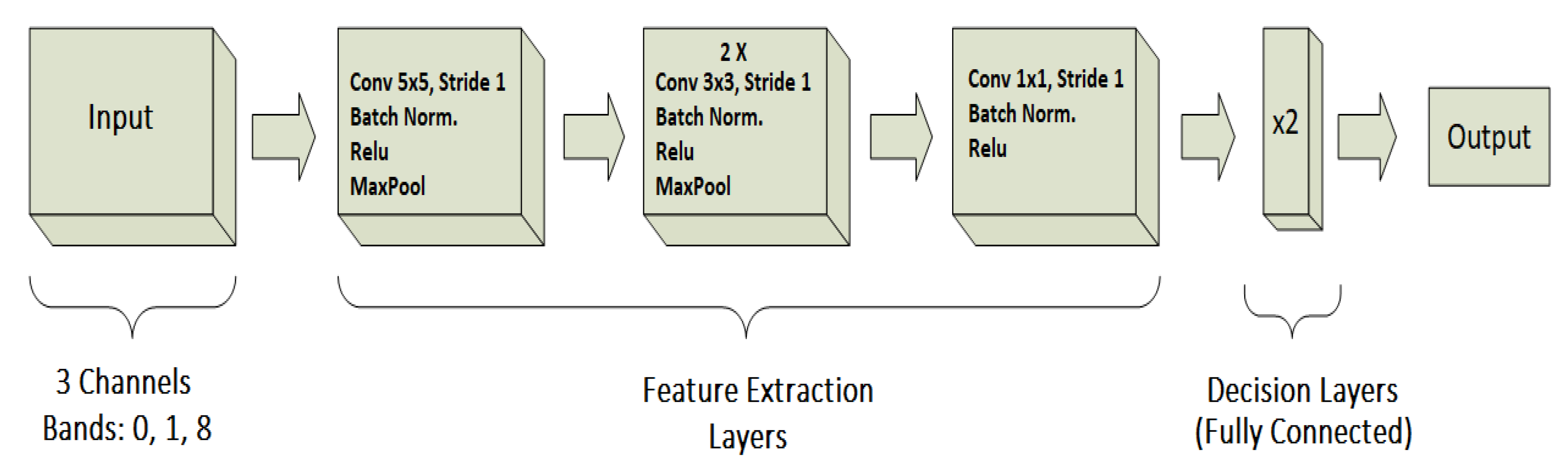
3.4.2. CloudScout Network Structure

The model is composed by two levels: feature extraction and decision, as shown in Figure 7.

The layers of the feature extraction level are used to discriminate different components of each image using convolutional layer with different kernel sizes and depth. This allows to separate clouds with respect to terrains, sea, sand, etc. Feature extraction level is composed by a convolutional size reduction layer followed by four group of three convolutional layers. Each group improves the generalization performance exploiting a sequence of kernels of $3\times 3$, $1\times 1$, $3\times 3$, which provides the same performance of a $5\times 5$ kernel, but they reduce the number of weights. Furthermore, the output given by the $1\times 1$ convolutional layer with the bias set to true represents a local pixel level classification [36]. In order to allow future upload of the network during the mission and to meet the model size requirement (less than 5 MB) a Global Max Pooling layer was exploited. It extracts the maximum value from each filter produced by the last convolutional layer of the feature extraction level.

The decision layer collects and assigns a value to the data produced by the Global Max Pooling in the feature extraction level.

The last layer is a softmax, which computes the probability of belonging to the first or second class from the output of the decision level. The training was performed in two steps:

• train the CNN model against the dataset with labels generated by using TH30 dataset to improve the recognition of the shape of the clouds;
• train the CNN model against the dataset with labels generated by using TH70 dataset to improve the accuracy of the decision layers.

One of the given requirement was to obtain FP number of 1% with respect to the given dataset without affecting the accuracy. Since accuracy and Receiver Operating Characteristic (ROC) analysis assume FP and False Negative (FN) results to be equally important, we decided to exploit the $F_2$ metrics. This metric is a particular case of the $F_{\beta }$ score, also known as the Sørensen–Dice coefficient or Dice Similarity Coefficient (DSC), defined in Equation (1).

$$F_{\beta }=(1+{\beta }^2)·\frac{precision·recall}{({\beta }^2·precision)+recall}$$

(1)

$$=\frac{(1+{\beta }^2)·TP}{(1+{\beta }^2)·TP+{\beta }^2·FN+FP}$$

This equation gives more relevance to FP errors than FN errors and allows to better estimate the influence of the FP within the network.

Moreover, to effectively reduce the number of FP during the training phase, we changed the standard Binary-Cross Entropy loss-function, shown in Equation (2), by doubling the penalty given in case of FP errors.

$$L(y,\widehat{y})=-\frac{1}{N}·\sum _{i=0}^N(y_i·log\left({\widehat{y}}_i\right)+2·(1-y_i)·log(1-{\widehat{y}}_i))$$

(2)

where y is the expected/labeled value, and $\widehat{y}$ is the predicted value.

This produced a network more prone to classify images as cloudless, effectively reducing the number of FP results at the expense of producing more FN ones. However, the increased number of FN results, does not pose a threat to the overall performance of the system thanks to the high value of accuracy of $92\%$ on the EoT as detailed in Section 4.

4. Results

In this Section, we show the results obtained from the CNN model described in Section 3.4 implemented on the EoT board featuring the Myriad 2 hardware accelerator.

As shown in

Table 3. Performance of the CloudScout model on the EoT board (Myriad 2).

ROC analysis:
TPR	0.83
FPR	0.02
False Positive	1.03 %
EoT board (Myriad 2) accuracy	92 %

and in

Table 4. Confusion matrix of the CloudScout model run on the entire dataset.

	Cloudy	Not Cloudy
Cloudy	32.5 %	1 (FP)%
Not Cloudy	6.8 (FN) %	59.7 %

we met all the requirements, described in Section 2, related to Accuracy and False Positive Rate. These results were obtained exploiting the entire 43,092 images contained in the dataset since the network quantization process could fully change the hyper-plane of the network. The network was trained by exploiting an initial learning rate of $lr=0.01$ and using an exponential decay computed as shown in Equation (3).

$$lr=l{r}_{old}·e^{-0.6·epoch}$$

(3)

where $lr$ is the new learning rate computed at each epoch, $l{r}_{old}$ is the learning rate used for the previous epoch, $epoch$ is the actual number of epoch, and $0.6$ is a constant chosen empirically. In

Table 5. Network characterization on EoT board (Myriad 2).

EoT board (Myriad 2) Inference Time	325 ms
Model memory footprint	2.1 MB
Power consumption per inference	1.8 W

the model characterization run on the EoT board is reported, taking into account inference time, power consumption per inference, and memory footprint. Furthermore, as preliminary described in Section 2, the 2.1 MB memory footprint allows uploading a new version of weights during the mission operation through telecommand allowing on-the-fly flexibility and improvements.

The CloudScout network has been also tested using a dataset of 24 images representing some critical environments with or without clouds. The critical dataset is composed of images taken by Sentinel-2 and elaborated following the same criteria used in Section 3.3. In particular, the 24 images contain very difficult classification problems due to the presence of salt lakes or snow mountains mixed with clouds. On this dataset, the CloudScout network achieves 67% accuracy with only 8 misclassified images against the 24 of the entire critical dataset. The obtained results are described in the Confusion Matrix described in

Table 6. Confusion matrix of the model with respect to the critical test set.

	Cloudy	Not Cloudy
Cloudy	2	2 (FP)
Not Cloudy	6 (FN)	14

. It is noted that the number of FN classifications is much higher than the FP owing to the unbalance of the loss function, described in Section 2, used during the training.

Some example of the images contained in the critical dataset are shown in Figure 8, Figure 9, Figure 10, Figure 11 and Figure 12. Each figure shows the radiance image obtained after the elaboration to represent a CloudScout 2 image, its RGB visible image, and the corresponding binary cloud mask which shows in white the cloudy pixels while in black the not cloudy ones. The binary mask was used as ground truth only to compute the number of cloudy pixels inside the image. Figure 8, Figure 9 and Figure 10, represent three of the most obvious wrong classifications while Figure 11 and Figure 12 are two examples of good classifications. Here we briefly give a justification for the wrong classification of three images:

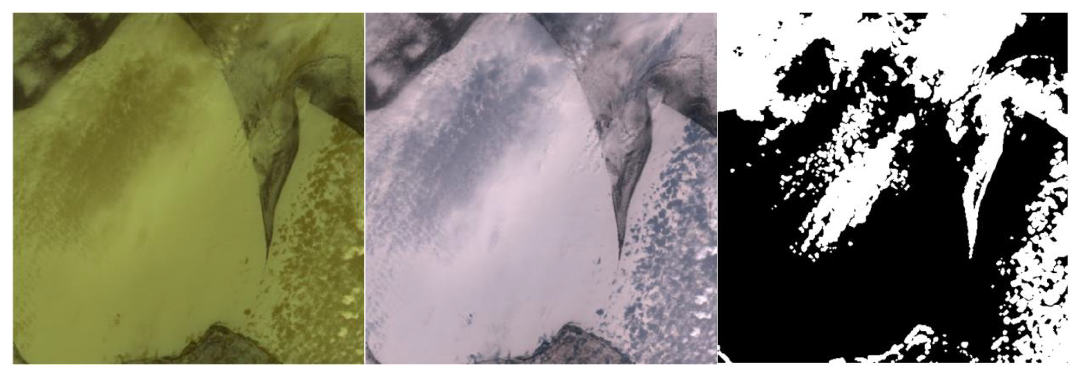
• In Figure 8 the network recognises ice as a continuum of the cloud. To avoid this behaviour, a possible solution could be to use a thermal band that provides high-quality cloud contours.
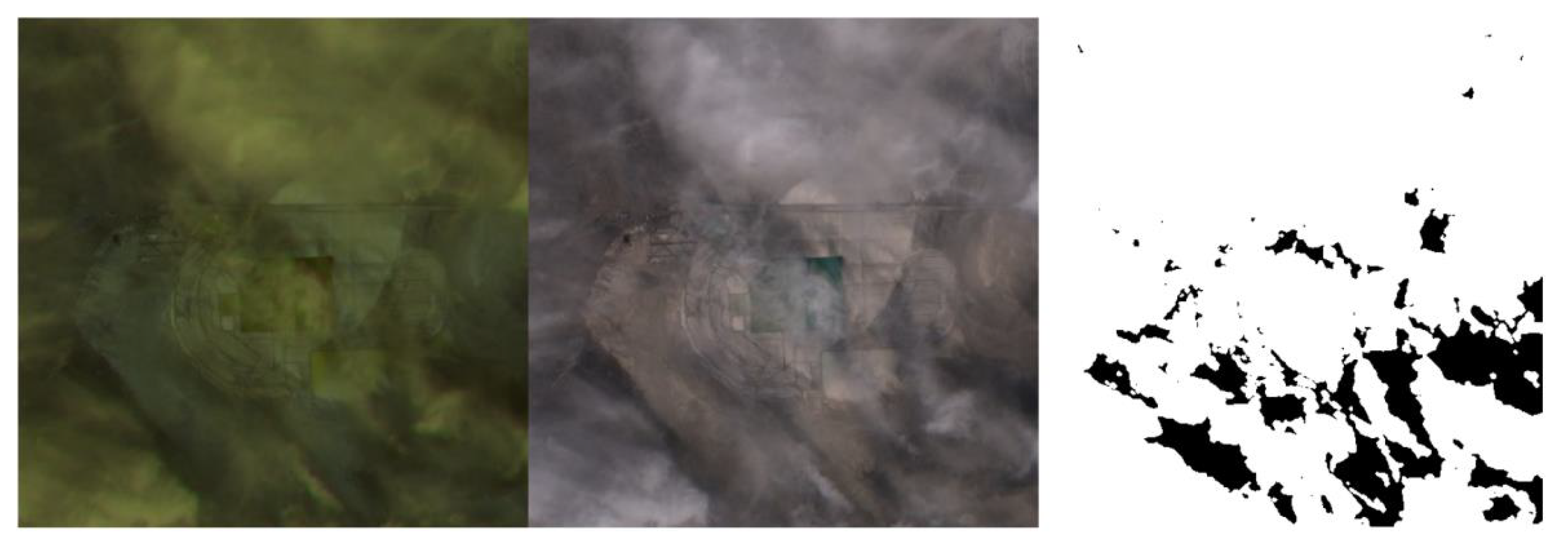
• The CloudScout network was not trained to recognise the fog, even if in some cases it could represent a big obstacle to visibility. This phenomenon is observable in Figure 9. Here, the image is fully covered by fog as further shown by the cloud mask, but our network does not interpret the fog as cloud obtaining, in fact, just a 1% probability of cloudiness in this picture.
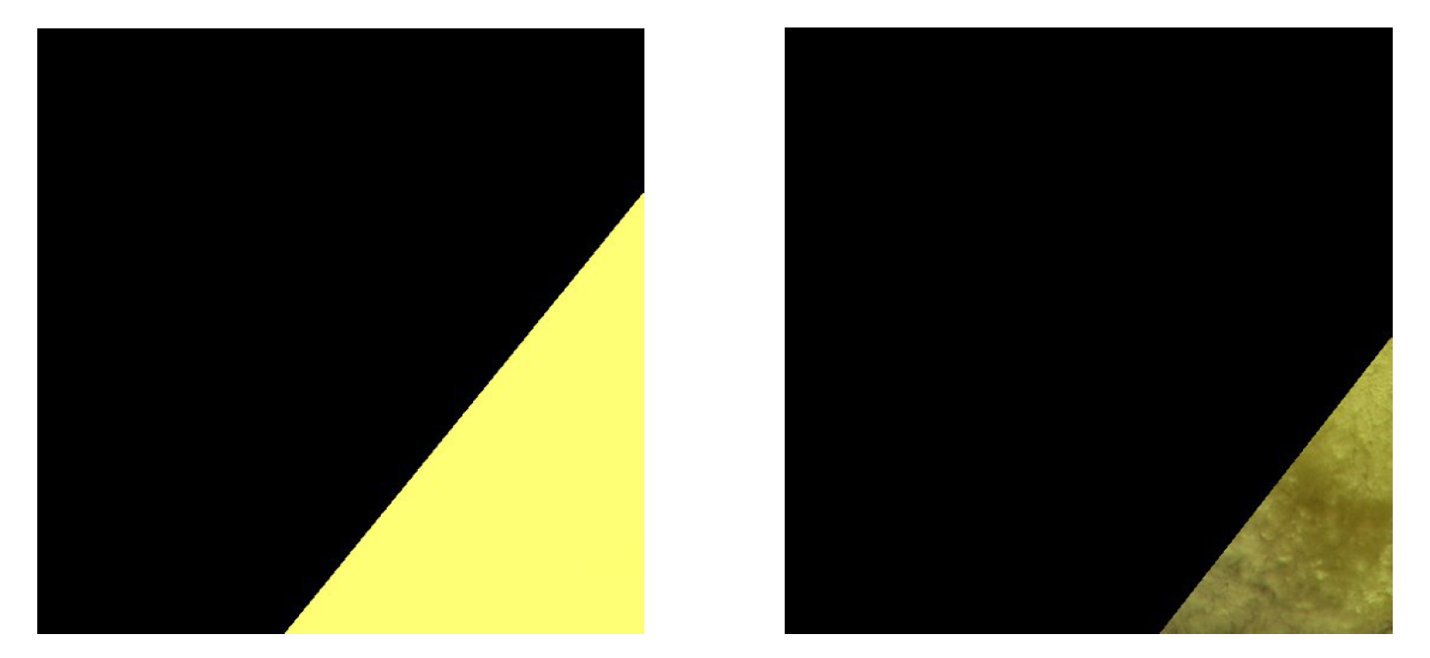
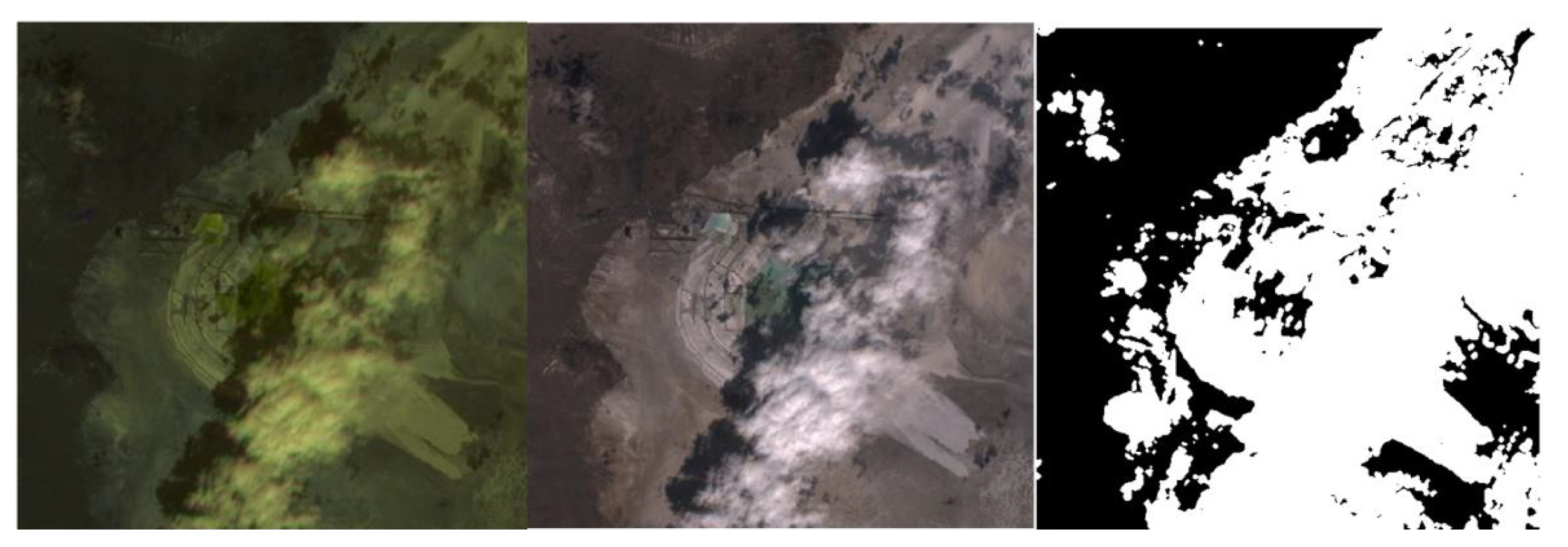
• Another reason for wrong classifications is the use of a fixed threshold to define an image cloudy or not. Indeed, as shown in Figure 10, the cloudiness inside the image is about 65%. This value is very close to the threshold selected for this project (70%). To achieve a better result for all the borderline cases should be useful to increase the granularity of the classification, developing a segmentation network.

Finally,

Table 7. The critical test set results.

Name	Clouds %	Prob. of Cloudiness % (Net Output)
Aral Sea clouds and ice Figure 8	35%	99 %
Bonneville clouds Figure 9	87%	1 %
Algeria mixed clouds and shadows	98%	0 %
Erie ice clouds Figure 10	65%	96 %
Pontchartrain clouds	72%	1 %
Amadeus January clouds	78%	1 %
Aral Sea clouds	87%	2 %
Aral Sea thin clouds	90%	0%
Aral Sea no clouds	0%	0%
Pontchartrain sun glint	3%	0%
Caspian sea cloud	64%	0%
Alps snow no clouds	9%	0%
Bonneville clouds shadows Figure 11	56%	1%
Greenland snow ice no-cloud	2%	18%
Alps snow cloud no-shadow	44%	12%
Amadeus no clouds	0%	0%
Alps snow cloud shadow	22%	0%
Greenland snow ice clouds	85%	99%
Amadeus no-clouds	3%	0%
Bonneville no clouds	29%	0%
Erie ice no-clouds	0%	9%
Amadeus clouds	99%	100%
Pontchartrain small clouds	14%	0%
Pontchartrain clouds over water Figure 12	66%	2%

shows the output details of the inferences performed on the critical dataset.

5. Discussion

The advantages and limitations of the proposed approach concerning several aspects are discussed in this Section:

• Relaxing Bandwidth limitations: as described in Section 1, the introduction of DNNs onboard Earth Observation satellites allows filtering data produced by sensors according to the Edge computing paradigm. In particular, cloud-covered images can be discarded mitigating bandwidth limitations. More detailed information on these aspects is provided in [6,7,8].
  However, producing a binary response (cloudy/not cloudy) leads to a complete loss of data when clouds are detected, preventing the applications of cloud removal techniques, described in [37,38,39]. Such approaches allow reconstructing the original contents by exploiting low-rank decomposition using temporal information of different images, spatial information of different locations, or frequency contents of other bands. Such methods are generally performed on ground because of their high complexity.
  To enable the use of these approaches and to the reduction of downlink data through filtering data on the edge, DNN-based approaches performing image segmentation can be exploited [40]. In this way, pixel-level information on the presence of clouds can be exploited to improve compression performance through the substitution of cloudy areas through completely white areas. In this way, the application of cloud removal techniques can be performed after data downlink.
  The implementation of a segmentation DNN for on-board cloud-detection represents a future work.
• Power-consumption/inference time: The use of DNNs allows leveraging modern COTS hardware accelerators featuring enhanced performance/throughput trade-offs compared to space-qualified components [6]. Table 5 shows the proposed model can perform an inference in 325 ms with an average power consumption of 1.8 W. Such reduced power consumption represents an important outcome for CubeSats, for which the limited power budget represents an additional limitation for downlink throughput [41].
• Training procedure: This work proposes to exploit a synthetic dataset for the training of the DNN model in view of the lack of data due by the novelty of the HyperScout 2 imager [11].
  Despite the functionality of the proposed approach has still to be demonstrated through the validation by means of HyperScout 2 data, the methodology described might be exploited in near future to realize a preliminary training of new applications used for novel technology for which a proper dataset is not available. Moreover, thanks to the possibility to reconfigure hardware accelerators for DNNs, the model can be improved after the launch thanks to a fine-tuning process performed through the actual satellite data [6].
• Cloud detection performance: There are different cloud detection techniques for satellite images, both at the pixel and image level. Yang at al. [42] divide the cloud detector techniques into three categories:

  -

  Threshold methods: some of the most known thresholding-based techniques are ISCPP [43], APOLLO [44], MODIS [45], ACCA [46], and some new methods which work well when ice and clouds coexist. However, these methods are very expensive for the CPU because of the application of several custom filters on the images. Hence, they are not good candidates to be used directly on-board.

  -

  Multiple image-based methods: Zhu and Woodcock [47] use multiple sequential images to overcome the limitations of thresholding-like algorithms. Again, processing this information requires an amount of power that is hardly available on board. In addition, this method requires the use of a large amount of memory.

  -

  Learning-base methods: these methods are the most modern. They exploit all the ML techniques such as Support Vector Machines (SVM) [48], Random Forest (RF) [49], and NN as our CloudScout or [42]. Contrary to SVM and RF methods, NNs have a standard structure that allows building ad-hoc accelerators able to speed up the inference process by reducing energy consumption.

All three categories provide an excellent solution for ground processing. However, the purpose of CloudScout is to provide reliable information directly on board, without requiring a huge amount of power. So, thanks to the technological advancement given by the EoT board, we developed a simple NN model that performs a hyperspectral image threshold directly on board. The needed to build a new custom model and do not exploit directly one taken from the literature is given by the limitation of the hardware itself. In fact, as described in Section 3.2, the accelerator has some hardware constraints that must be considered in order to obtain a valid result.

6. Conclusions

The Phi-sat mission and in particular Hyperscout 2 is a nano-sat system with the aim to demonstrate the possibility of using DNN in space, by exploiting COTS hardware accelerators directly on-board, such as the Myriad-2 VPU. Moreover, the reconfigurability provided by these devices enables the update of DNN models on the fly, allowing to improve the model performance exploiting new data acquired during the mission. Furthermore, thanks to the intrinsic modularity of such DNN models, it would be possible to change the mission goals during the mission life.

This may represent the beginning of a new era of re-configurable smart satellites equipped by programmable hardware accelerator (such as the Myriad 2) enabling the on-demand paradigm at payload level [6].

As described by [6], this fact would enable a significant cost reduction due to satellite design or even satellite platform reuse.

Other advantages are related to the smart use of transmission bandwidth that represents one of the main concern in nearly future in view of the growing number of satellites and the increasing resolution of on-board sensors [6,8]. The efficacy of AI and in particular of CNN for this goal will be demonstrated by the results of the HyperScout-2, which might represent a precursor for this new smart satellite era. Indeed, such results demonstrate that exploiting a CNN running on the Intel Movidius Myriad 2 we are able to detect with a 92% accuracy, 1.8W of power consumption, and 2.1 MB of memory footprint the cloudiness of hyperspectral images directly on board the satellite.

References

1. Sweeting, M.N. Modern small satellites-changing the economics of space. Proc. IEEE 2018, 106, 343–361. [Google Scholar] [CrossRef]
2. Madry, S.; Martinez, P.; Laufer, R. Conclusions and Top Ten Things to Know About Small Satellites. In Innovative Design, Manufacturing and Testing of Small Satellites; Springer: Berlin, Germany, 2018; pp. 105–111. [Google Scholar]
3. Shi, W.; Cao, J.; Zhang, Q.; Li, Y.; Xu, L. Edge computing: Vision and challenges. IEEE Internet Things J. 2016, 3, 637–646. [Google Scholar] [CrossRef]
4. Li, H.; Zheng, H.; Han, C.; Wang, H.; Miao, M. Onboard spectral and spatial cloud detection for hyperspectral remote sensing images. Remote Sens. 2018, 10, 152. [Google Scholar] [CrossRef] [Green Version]
5. Hagolle, O.; Huc, M.; Pascual, D.V.; Dedieu, G. A multi-temporal method for cloud detection, applied to FORMOSAT-2, VENμS, LANDSAT and SENTINEL-2 images. Remote Sens. Environ. 2010, 114, 1747–1755. [Google Scholar] [CrossRef] [Green Version]
6. Furano, G.; Meoni, G.; Dunne, A.; Moloney, D.; Ferlet-Cavrois, V.; Tavoularis, A.; Byrne, J.; Buckley, L.; Psarakis, M.; Voss, K.O.; et al. Towards the use of Artificial Intelligence on the Edge in SpaceSystems: Challeng-es and Opportunities. IEEE Aerosp. Electron. Syst. 2020. forthcoming. [Google Scholar]
7. Kothari, V.; Liberis, E.; Lane, N.D. The Final Frontier: Deep Learning in Space. In Proceedings of the 21st International Workshop on Mobile Computing Systems and Applications, Austin, TX, USA, 3–4 March 2020; pp. 45–49. [Google Scholar]
8. Denby, B.; Lucia, B. Orbital Edge Computing: Nanosatellite Constellations as a New Class of Computer System. In Proceedings of the Twenty-Fifth International Conference on Architectural Support for Programming Languages and Operating Systems, Lausanne, Switzerland, 16–20 March 2020; pp. 939–954. [Google Scholar]
9. Deniz, O.; Vallez, N.; Espinosa-Aranda, J.; Rico-Saavedra, J.; Parra-Patino, J.; Bueno, G.; Moloney, D.; Dehghani, A.; Dunne, A.; Pagani, A.; et al. Eyes of Things. Sensors 2017, 17, 1173. [Google Scholar] [CrossRef] [Green Version]
10. Pastena, M.; Domínguez, B.C.; Mathieu, P.P.; Regan, A.; Esposito, M.; Conticello, S.; Dijk, C.V.; Vercruyssen, N. ESA Earth Observation Directorate NewSpace initiatives. Session V. 2019. Available online: https://digitalcommons.usu.edu/smallsat/2019/all2019/92/ (accessed on 7 July 2020).
11. Esposito, M.; Conticello, S.S.; Pastena, M.; Carnicero Domínguez, B. HyperScout-2: Highly Integration of Hyperspectral and Thermal Sensing for Breakthrough In-Space Applications. In Proceedings of the ESA Earth Observation ϕ-Week 2019, Frascati, Italy, 9–13 September 2019. [Google Scholar]
12. Esposito, M.; Conticello, S.; Pastena, M.; Domínguez, B.C. In-orbit demonstration of artificial intelligence applied to hyperspectral and thermal sensing from space. In CubeSats and SmallSats for Remote Sensing III; International Society for Optics and Photonics: San Diego, CA, USA, 2019; Volume 11131, p. 111310C. [Google Scholar]
13. Benelli, G.; Meoni, G.; Fanucci, L. A low power keyword spotting algorithm for memory constrained embedded systems. In Proceedings of the 2018 IFIP/IEEE International Conference on Very Large Scale Integration (VLSI-SoC), Verona, Italy, 8–10 October 2018; pp. 267–272. [Google Scholar]
14. Reuther, A.; Michaleas, P.; Jones, M.; Gadepally, V.; Samsi, S.; Kepner, J. Survey and benchmarking of machine learning accelerators. arXiv 2019, arXiv:1908.11348. [Google Scholar]
15. Wang, Y.E.; Wei, G.Y.; Brooks, D. Benchmarking TPU, GPU, and CPU platforms for deep learning. arXiv 2019, arXiv:1907.10701. [Google Scholar]
16. Jouppi, N.P.; Young, C.; Patil, N.; Patterson, D.; Agrawal, G.; Bajwa, R.; Bates, S.; Bhatia, S.; Boden, N.; Borchers, A.; et al. In-datacenter performance analysis of a tensor processing unit. In Proceedings of the 44th Annual International Symposium on Computer Architecture, Toronto, ON, Canada, 24–28 June 2017; pp. 1–12. [Google Scholar]
17. Abadi, M.; Barham, P.; Chen, J.; Chen, Z.; Davis, A.; Dean, J.; Devin, M.; Ghemawat, S.; Irving, G.; Isard, M.; et al. Tensorflow: A system for large-scale machine learning. In Proceedings of the 12th USENIX Symposium on Operating Systems Design and Implementation (OSDI 16), Savannah, GA, USA, 2–4 November 2016; pp. 265–283. [Google Scholar]
18. Nickolls, J.; Dally, W.J. The GPU Computing Era. IEEE Micro 2010, 30, 56–69. [Google Scholar] [CrossRef]
19. Dinelli, G.; Meoni, G.; Rapuano, E.; Benelli, G.; Fanucci, L. An FPGA-Based Hardware Accelerator for CNNs Using On-Chip Memories Only: Design and Benchmarking with Intel Movidius Neural Compute Stick. Int. J. Reconfigurable Comput. 2019, 2019, 7218758. [Google Scholar] [CrossRef] [Green Version]
20. Baze, M.P.; Buchner, S.P.; McMorrow, D. A digital CMOS design technique for SEU hardening. IEEE Trans. Nucl. Sci. 2000, 47, 2603–2608. [Google Scholar] [CrossRef]
21. Sterpone, L.; Azimi, S.; Du, B. A selective mapper for the mitigation of SETs on rad-hard RTG4 flash-based FPGAs. In Proceedings of the 2016 16th European Conference on Radiation and Its Effects on Components and Systems (RADECS), Bremen, Germany, 19–23 September 2016; pp. 1–4. [Google Scholar]
22. Lowe, D.G. Distinctive Image Features from Scale-Invariant Keypoints. Int. J. Comput. Vis. 2004, 60, 91–110. [Google Scholar] [CrossRef]
23. Barry, B.; Brick, C.; Connor, F.; Donohoe, D.; Moloney, D.; Richmond, R.; O’Riordan, M.; Toma, V. Always-on Vision Processing Unit for Mobile Applications. IEEE Micro 2015, 35, 56–66. [Google Scholar] [CrossRef]
24. Rivas-Gomez, S.; Pena, A.J.; Moloney, D.; Laure, E.; Markidis, S. Exploring the vision processing unit as co-processor for inference. In Proceedings of the 2018 IEEE International Parallel and Distributed Processing Symposium Workshops (IPDPSW), Vancouver, BC, Canada, 21–25 May 2018; pp. 589–598. [Google Scholar]
25. Myriad2VPU. Available online: https://www.movidius.com/myriad2 (accessed on 7 July 2020).
26. Antonini, M.; Vu, T.H.; Min, C.; Montanari, A.; Mathur, A.; Kawsar, F. Resource Characterisation of Personal-Scale Sensing Models on Edge Accelerators. In Proceedings of the First International Workshop on Challenges in Artificial Intelligence and Machine Learning for Internet of Things, New York, NY, USA, 16–19 November 2019; pp. 49–55. [Google Scholar]
27. Li, W.; Liewig, M. A Survey of AI Accelerators for Edge Environment. In World Conference on Information Systems and Technologies; Springer: Berlin, Germany, 2020; pp. 35–44. [Google Scholar]
28. Deschamps, P.; Herman, M.; Tanre, D. Definitions of atmospheric radiance and transmittances in remote sensing. Remote Sens. Environ. 1983, 13, 89–92. [Google Scholar] [CrossRef]
29. Sinergise Ltd. Available online: https://www.sinergise.com/en (accessed on 7 July 2020).
30. Intel Movidius SDK. Available online: https://movidius.github.io/ncsdk/ (accessed on 7 July 2020).
31. Jia, Y.; Shelhamer, E.; Donahue, J.; Karayev, S.; Long, J.; Girshick, R.; Guadarrama, S.; Darrell, T. Caffe: Convolutional Architecture for Fast Feature Embedding. arXiv 2014, arXiv:1408.5093. [Google Scholar]
32. Drusch, M.; Del Bello, U.; Carlier, S.; Colin, O.; Fernandez, V.; Gascon, F.; Hoersch, B.; Isola, C.; Laberinti, P.; Martimort, P.; et al. Sentinel-2: ESA’s optical high-resolution mission for GMES operational services. Remote Sens. Environ. 2012, 120, 25–36. [Google Scholar] [CrossRef]
33. Hecht-Nielsen, R. Theory of the backpropagation neural network. In Neural Networks for Perception; Elsevier: Amsterdam, The Netherlands, 1992; pp. 65–93. [Google Scholar]
34. Hubara, I.; Courbariaux, M.; Soudry, D.; El-Yaniv, R.; Bengio, Y. Quantized neural networks: Training neural networks with low precision weights and activations. J. Mach. Learn. Res. 2017, 18, 6869–6898. [Google Scholar]
35. Krishnamoorthi, R. Quantizing deep convolutional networks for efficient inference: A whitepaper. arXiv 2018, arXiv:1806.08342. [Google Scholar]
36. Lin, M.; Chen, Q.; Yan, S. Network in network. arXiv 2013, arXiv:1312.4400. [Google Scholar]
37. Ji, T.Y.; Yokoya, N.; Zhu, X.X.; Huang, T.Z. Nonlocal tensor completion for multitemporal remotely sensed images’ inpainting. IEEE Trans. Geosci. Remote Sens. 2018, 56, 3047–3061. [Google Scholar] [CrossRef]
38. Kang, J.; Wang, Y.; Schmitt, M.; Zhu, X.X. Object-based multipass InSAR via robust low-rank tensor decomposition. IEEE Trans. Geosci. Remote Sens. 2018, 56, 3062–3077. [Google Scholar] [CrossRef] [Green Version]
39. Chen, Y.; He, W.; Yokoya, N.; Huang, T.Z. Blind cloud and cloud shadow removal of multitemporal images based on total variation regularized low-rank sparsity decomposition. ISPRS J. Photogramm. Remote Sens. 2019, 157, 93–107. [Google Scholar] [CrossRef]
40. Badrinarayanan, V.; Kendall, A.; Cipolla, R. Segnet: A deep convolutional encoder-decoder architecture for image segmentation. IEEE Trans. Pattern Anal. Mach. Intell. 2017, 39, 2481–2495. [Google Scholar] [CrossRef] [PubMed]
41. Selva, D.; Krejci, D. A survey and assessment of the capabilities of Cubesats for Earth observation. Acta Astronaut. 2012, 74, 50–68. [Google Scholar] [CrossRef]
42. Yang, J.; Guo, J.; Yue, H.; Liu, Z.; Hu, H.; Li, K. Cdnet: Cnn-based cloud detection for remote sensing imagery. IEEE Trans. Geosci. Remote Sens. 2019, 57, 6195–6211. [Google Scholar] [CrossRef]
43. Rossow, W.B.; Garder, L.C. Cloud detection using satellite measurements of infrared and visible radiances for ISCCP. J. Clim. 1993, 6, 2341–2369. [Google Scholar] [CrossRef]
44. Gesell, G. An algorithm for snow and ice detection using AVHRR data An extension to the APOLLO software package. Int. J. Remote Sens. 1989, 10, 897–905. [Google Scholar] [CrossRef]
45. Wei, J.; Sun, L.; Jia, C.; Yang, Y.; Zhou, X.; Gan, P.; Jia, S.; Liu, F.; Li, R. Dynamic threshold cloud detection algorithms for MODIS and Landsat 8 data. In Proceedings of the 2016 IEEE International Geoscience and Remote Sensing Symposium (IGARSS), Beijing, China, 10–15 July 2016; pp. 566–569. [Google Scholar]
46. Zhong, B.; Chen, W.; Wu, S.; Hu, L.; Luo, X.; Liu, Q. A cloud detection method based on relationship between objects of cloud and cloud-shadow for Chinese moderate to high resolution satellite imagery. IEEE J. Sel. Top. Appl. Earth Obs. Remote Sens. 2017, 10, 4898–4908. [Google Scholar] [CrossRef]
47. Zhu, Z.; Woodcock, C.E. Automated cloud, cloud shadow, and snow detection in multitemporal Landsat data: An algorithm designed specifically for monitoring land cover change. Remote Sens. Environ. 2014, 152, 217–234. [Google Scholar] [CrossRef]
48. Latry, C.; Panem, C.; Dejean, P. Cloud detection with SVM technique. In Proceedings of the 2007 IEEE International Geoscience and Remote Sensing Symposium, Barcelona, Spain, 23–28 July 2007; pp. 448–451. [Google Scholar]
49. Deng, J.; Wang, H.; Ma, J. An automatic cloud detection algorithm for Landsat remote sensing image. In Proceedings of the 2016 4th International Workshop on Earth Observation and Remote Sensing Applications (EORSA), Guangzhou, China, 4–6 July 2016; pp. 395–399. [Google Scholar]
Figure 1. Example of hyperspectral Cube.
Remotesensing 12 02205 g001
Figure 2. Sentinel Hub results compared with the main cloud detector algorithms [29].
Remotesensing 12 02205 g002
Figure 3. Example of incomplete images found in our dataset.
Remotesensing 12 02205 g003
Figure 4. Example of images with not correctly aligned bands found in our dataset.
Remotesensing 12 02205 g004
Figure 5. Histogram representing the cloudiness distribution in our dataset.
Remotesensing 12 02205 g005
Figure 6. Iterative approach used to select the right network.
Remotesensing 12 02205 g006
Figure 7. The CloudScout model block diagram.
Remotesensing 12 02205 g007
Figure 8. Aral sea clouds and ice; radiance image, RGB image, cloud mask. False Positive case.
Remotesensing 12 02205 g008
Figure 9. Bonneville clouds; radiance image, RGB image, cloud mask. False Negative case.
Remotesensing 12 02205 g009
Figure 10. Erie ice and clouds; radiance image, RGB image, cloud mask. False Positive case.
Remotesensing 12 02205 g010
Figure 11. Bonneville clouds and shadows; radiance image, RGB image, cloud mask.
Remotesensing 12 02205 g011
Figure 12. Pontchartrain clouds over water; radiance image, RGB image, cloud mask.
Remotesensing 12 02205 g012