Article

Extreme Events of Precipitation over Complex Terrain Derived from Satellite Data for Climate Applications: An Evaluation of the Southern Slopes of the Pyrenees

by
Andrés Navarro
*,
Eduardo García-Ortega
,
Andrés Merino
and
José Luis Sánchez
Atmospheric Physics Group (GFA), Environmental Institute (IMA), Universidad de León, 24071 León, Spain
*
Author to whom correspondence should be addressed.
Remote Sens. 2020, 12(13), 2171; https://doi.org/10.3390/rs12132171
Submission received: 7 June 2020 / Revised: 1 July 2020 / Accepted: 5 July 2020 / Published: 7 July 2020
(This article belongs to the Special Issue Precipitation and Water Cycle Measurements Using Remote Sensing)

Abstract

:
Estimating extreme precipitation events over complex terrain is challenging but crucial for evaluating the performance of climate models for the present climate and expected changes of the climate in the future. New satellites operating in the microwave wavelengths have started to open new opportunities for performing such estimation at adequate temporal and spatial scales and within sensible error limits. This paper illustrates the feasibility and limits of estimating precipitation extremes from satellite data for climatological applications. Using a high-resolution gauge database as ground truth, it was found that global precipitation measurement (GPM) constellation data can provide valuable estimates of extreme precipitation over the southern slopes of the Pyrenees, a region comprising several climates and a very diverse terrain (a challenge for satellite precipitation algorithms). Validation using an object-based quality measure showed reasonable performance, suggesting that GPM estimates can be advantageous reference data for climate model evaluation.

Graphical Abstract

1. Introduction

Extreme precipitation events (EPEs) have devastating effects on human society. They are responsible for a substantial number of natural disasters, including landslides and flash floods [1]. Consequently, accurate estimates of heavy rainfall are essential for the risk monitoring of these natural hazards. In this sense, in situ observation, satellite-based measurements, model outputs, and reanalysis datasets are very beneficial because they provide continuous spatial and temporal coverage of EPEs.
Gridded products derived from rain gauges are commonly used to evaluate EPEs because of the advantages of their direct measurement. However, products derived from point-scale gauge observations can greatly deviate from areal precipitation, especially when the network is too sparse [2]. This issue is crucial in complex areas where sharp gradients play a key role in the distribution of precipitation. Compared with rain gauge data, satellite-derived precipitation products (SPPs) provide global and consistent measurement of precipitation, filling the gaps of in situ observations [3,4]. One of the most recent SPPs is the integrated multi-satellite retrievals from global precipitation measurement (IMERG) [5]. The IMERG product results from the combination of retrievals from multiple satellites and has emerged as a powerful tool for natural hazard monitoring [6], including EPEs [7,8,9,10,11]. IMERG is not only used in hazard monitoring but also in climate research. For example, Zhou et al. [12] constructed a global database of EPEs that allows analyses of many event-based precipitation characteristics that conventional datasets are unable to support. Despite its benefits, SPPs are not immune to errors and suffer from several limitations, including sensor sensitivity, algorithm limitations, and merging errors, among others [13,14,15].
Other sources for evaluating EPEs are reanalyses and climate models. Reanalyses are considered the best physically consistent estimates of the atmospheric state, and include observations through data assimilation from multiple sources. They have the potential to describe weather conditions over a longer period than satellite-derived observations and to produce high-resolution data relative to gauge observations. For those reasons, reanalyses are useful tools for reconstructing precipitation patterns and real-time monitoring [16,17]. On the other hand, numerical models are often used for forecast purposes [18,19,20]. In this sense, climatologists use global climate models (GCMs) to assess future global and regional trends of extreme precipitation [21,22,23]. However, both approaches have important drawbacks. For example, the reliability of reanalyses depends on the quality of the observational data and performance of the numerical model. Consequently, agreement between different reanalysis datasets is not frequent [16,24]. For models, coarse spatial resolutions lead to less accurate parameterizations that are unable to resolve heavy rainfall [25,26,27,28,29].
There are several studies comparing the strengths and limitations of gridded precipitation products for EPE detection. Some of them intercompare products on a regional basis [30,31,32,33,34] while others take a global approach [32,35,36,37]. However, few studies have attempted to evaluate the potential utility of IMERG for the study of EPEs in complex terrain [38,39], and none of them have focused on climate applications for the southern slopes of the Pyrenees.
This work aimed to answer the following questions: (1) From an object-based perspective, how well is very intense precipitation represented in IMERG products? (2) Could IMERG be a reliable alternative to gauge-derived products and reanalysis datasets for evaluating extreme precipitation? To address these questions, we focused on complex terrain in the northeastern Iberian Peninsula. This area is challenging because it is frequently affected by EPEs and has strong vulnerability to climate change [18,40,41]. However, it is equipped with a robust rain gauge network that furnishes reference data. The study included standard metrics and other object-based statistics that measure the potential utility of IMERG in evaluating certain characteristics of extreme rainfall not addressed by previous studies.
This paper is organized as follows. In Section 2, we introduce the study area, datasets, and methodology. Section 3 evaluates the performance of IMERG, focusing on different parameters, such as the structure, location, intensity, seasonality, and climate zone. Section 4 summarizes the main conclusions.

2. Study Area, Data, and Methodology
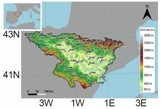
2.1. Study Area

The present study focuses on the western Mediterranean, more precisely on the NE of Iberian Peninsula (Figure 1). EPEs in this area occur mainly in autumn and are caused by orographic precipitation, mesoscale convective systems (MCSs), and frontal systems. The synoptic-scale processes that favor EPEs in this region have been extensively investigated [42,43,44,45] and multiple case studies can be found in the scientific literature [46,47,48,49,50,51].
The study area comprises extends over ~85,000 km2, covering the northeast of the Iberian Peninsula (Figure 1). It spans latitudes 40°33′ N–43°03′ N and longitudes 4°35′ W–1°85′ E, with altitudes from 0 to 3300 m. Most of the domain is covered by the Ebro River basin, which is surrounded by a set of mountainous ranges, the Pyrenees in the north, Duero Mountains in the southwest, and the Teruel System in the southeast [52]. The area is influenced by large-scale atmospheric circulations originating from the North Atlantic and the Mediterranean Sea [53]. The impact of these circulations is modulated by orographically complex terrain [54]. Consequently, MCSs are frequent in the middle and lower parts of the basin [55], in contrast to the stratiform rainfall of the northwest.
Precipitation estimates in the study area is a difficult task for both rain gauges and satellite products. On the one hand, the coverage of stations over mountains is usually low, with large areas with little or no information. Furthermore, the measurement of rainfall at high elevation is more susceptible to wind, evaporative loss, and siting [56,57]. On the other hand, satellite-based precipitation products, such as IMERG, are also prone to uncertainties. For example, rainfall intensity in warm orographic clouds cannot be accurately captured by infrared (IR) retrievals [58]. The Passive microwave (PMW) algorithms have also important limitations because of the emissivity of land surface. This bias is more pronounced during extreme events and over mountainous regions [59,60,61].
The study area embraces four climate zones (Table 1). Semiarid and Mediterranean regions cover almost 40% of the domain and include the dry lowlands of the Ebro basin (BSk) and territories near the Ebro river mouth (Csa and Csb). The temperate region (Cfa and Cfb) is an area of medium altitude that surrounds the mountain ranges of the domain. Cold climates (Dfb and Dfc) are restricted to areas of high altitude in the Pyrenees.
Figure 2 shows climate zones and boxplots of the monthly precipitation at eight selected locations for the 2008–2018 period. There is strong contrast observed between the dry southeast (<50 mm/month), humid west (50–80 mm/month), and Pyrenees (>80 mm/month). Outliers are mostly in spring and autumn, suggesting events of extreme precipitation.

2.2. Datasets

2.2.1. Gauge Dataset and Quality Control

The Automatic Hydrological Information System of the Ebro Hydrographic Confederation (SAIH-Ebro) comprises 367 rain gauge stations covering the period 2008–2018 (Figure 1; white dots). The use of this in situ observation network instead of the meteorological network of the Spanish Meteorological Agency (AEMET) is advantageous because the former is entirely independent of satellite and reanalysis products. Additionally, data from SAIH-Ebro have been used in previous research [62,63,64,65].
The original time series of observations were reconstructed using the R package reddPrec [66], following the methodology described in Serrano-Notivoli et al. [67]. Reconstruction was based on two steps: (1) Quality Control checks (QC) to detect and remove suspect data; and (2) estimation of daily precipitation for all observations with missing values on all days for the entire cleaned dataset, based on the nearest observations. The results of QC are available in the Supplementary Material (S2.1).

2.2.2. Grid Reconstruction

Products distributed on regular grids, whether satellite data, gauge-derived datasets, or reanalysis products, are currently used in most climatological studies. Some gridded datasets are derived from point-wise measurements, but others are directly computed at the cell level, such as model output. These products offer several advantages over point data: They are easy to compare with other products; they allow advanced spatial analysis; and they are useful for model validation, among other tasks.
Gridded products derived from rain gauges are powerful instruments to evaluate precipitation estimates but they are subjected to spatial interpolation to convert point-scale measurements into areal estimates [68]. Interpolation brings additional uncertainties and the quality of the interpolated precipitation at pixels without gauges is typically lower than that at pixels with gauges [69]. Therefore, a dense network of rain gauge stations is critical to minimize uncertainties in a gridded product.
ReddPrec includes a function for grid reconstruction that creates generalized linear models to compute the reference values (RVs) using precipitation data (occurrence and magnitude) of the 10 nearest neighbors as the dependent variable and geographic information of each station (latitude, longitude, and altitude) as independent variables. ReddPrec uses a unique and independent model for each grid point and day [67]. The result was a high-resolution (0.1° × 0.1°) gridded daily precipitation dataset from 2008 to 2018.
Two types of parameters were calculated to evaluate the performance of the interpolation method, i.e., the measurement of errors in the reconstructed data and a sensitivity test for intense precipitation. The interpolated data were validated against 34 rain gauge stations provided by AEMET (Figure 1; black dots).
Figure 3 (top) shows the mean absolute error (MAE) at the precipitation gauges and their corresponding grid cells. The boxplots show good results at the monthly scale. The median (red line) in the MAE for all cases (top center) is <0.3 mm/day and slightly increases on days with precipitation (top right). Another important test is the ability of the product to capture rainfall intensity. This was evaluated by the R10mm (R20mm) index, which represents the number of days in a month for which precipitation exceeded 10 mm (20 mm). Agreement between the interpolated field and AEMET is clear in both cases, although there is slight underestimation for gridded data (Figure 3 bottom). The Supplementary Material (S2.1, S2.2, S2.3, and S2.4) includes more metrics about grid validation.

2.2.3. Satellite Datasets

IMERG is a precipitation dataset with a 30-min temporal resolution and 0.1° × 0.1° spatial resolution [5]. IMERG combines retrievals from passive microwave observations with infrared precipitation estimates to produce a quasi-global homogeneous precipitation product based only on satellite data. IMERG also includes retrievals from the GPM Core Observatory, allowing the detection of light rain and falling snow [6].
The latest version (IMERG v06b) includes several important updates. The biggest change is the switch from geosynchronous IR to numerical model data from MERRA-2 and GEOS FP for the derivation of motion vectors used to propagate the PMW precipitation observations [70]. This change was motivated by two reasons: Discrepancies between cloud-top motion and precipitation motion and the extension of IMERG coverage to the poles.
We used three IMERG v06b level-3 estimates of precipitation, the Early Run (IMERG-E), Late Run (IMERG-L), and Final Run (IMERG-F). Early and late products are conceptually the same but differ in their latency (4-h vs. 12-h lag) and how the IR data is folded into the microwave estimate. IMERG-E and IMERG-L are designed for near real-time applications, whereas IMERG-F is designed for research purposes. The final product (IMERG-F) incorporates monthly observed data from the Global Precipitation Climatology Centre (GPCC) dataset, which is derived from ~6700 stations worldwide [71]. IMERG-F is available after a two-month delay.

2.2.4. Reanalysis Dataset

Reanalysis combines model data with ground and satellite observations to generate a globally complete and consistent dataset using the laws of physics. It produces data that go back several decades, providing an accurate description of the past climate. The European Centre for Medium-Range Weather Forecasts recently released a new generation of reanalysis products (ERA5 and ERA5-Land) that replaced previous products [72]. ERA5-Land (ERA5-L hereafter) [73] is a replicate of the land component of ERA5 reanalysis but with a series of improvements making it more accurate for land-surface applications, such as flood or drought analysis. In particular, ERA5-L runs at an enhanced spatial resolution (0.1° vs. 0.3° in ERA5) with a one-hour temporal resolution. Observations indirectly influence ERA5-L through the atmospheric forcing of ERA5. The precipitation output from ERA5-L is the sum of large-scale and convective precipitation.
Reanalysis datasets are not immune to errors and their performance depends on several factors: The quality and availability of observations, shortcomings in the assimilation methodology, and uncertainties derived from models [74,75]. These limitations became more relevant over mountains [76]. Table 2 summarizes the datasets used in our study.

2.3. Methodology

2.3.1. Extreme Precipitation Events (EPEs)

An EPE was defined by the R99p index [77]. R99p is a widely used index created by the Expert Team on Climate Change and Detection Indices for identifying extremely wet days. An advantage of this metric is that the parameter depends on the distribution of precipitation at each location and thereby allows comparisons between different climate zones [78].
Cases were selected after reconstructing the 10-year time series of precipitation, which served as a base period for percentile calculation. The R99p is calculated based on daily precipitation on wet days (days with daily precipitation ≥ 1 mm). The R99p must be reached by at least 10 rain gauge stations in the domain. In total, 55 cases were selected.
Table 3 shows the complete list of cases filtered by date, maximum rainfall, climate region, and coordinates. Most cases are in the northern portion of the domain, others along the Ebro valley, and a few in the south (see Supplementary Material S1 for maps).

2.3.2. Metrics

We assessed the performance of IMERG using both statistical and graphical methods (see Table 4 for details). The standard metrics used include MAE, relative bias (RB), probability density functions (PDFs), and the correlation coefficient (CC). MAE and RB highlight differences between datasets, whereas CC is a measure of the match between reference data and precipitation estimates.
The structure-amplitude-location method (SAL) [79] evaluates precipitation fields by identifying objects in both a predicted and observed field at a given time, and decomposing errors into three components. The power of SAL lies in its ability to discriminate between errors, i.e., structure (S), amplitude (A), and location (L). The structural component S considers the gradient around an object and its size. Component A considers domain-wide accumulation. The L component combines information about the distance between predicted and observed mass centers and the error of a weighted average distance between the precipitation object centers of mass. A perfect forecast is characterized by zero values for all three SAL components.

3. Results and Discussion

3.1. Standard Evaluation of Extreme Rainfall

Standard comparisons for the 55 cases were performed against the gauge-derived dataset. In general, reanalysis and IMERG-F showed good agreement with the rain gauge data (see S3.1 and S3.5 for a complete comparison). Conversely, the early and late versions of IMERG overestimated very intense precipitation rates (≥100 mm/day). This issue can be clearly observed in Figure 4 (second and fifth columns) and the Supplementary Material (S3.1, S3.2, S3.3, S3.4, and S3.5).
Another interesting disagreement is with light rain detection (fourth column). IMERG products had problems in detecting weak precipitation (≤1 mm) because of the sensitivity of the satellite sensors, but this issue is not crucial in the analysis of EPEs [80,81]. For reanalysis data, the sharp gradient between rain and no-rain areas is poorly represented (third and fourth columns). A reason that may explain this issue is that sharp gradients and discontinuities are always difficult to model in systems of partial differential equations [82].
A closer look at other metrics reveal new issues partially hidden in the previous selection. Figure 5 (left) compares the PDF for all cases. There is a problem common to the ERA5-L and IMERG products; both were unable to reproduce the peak of light rain observed by rain gauges. Two more problems were found in the reanalysis data, an overestimation of pixels with moderate rain rate (≥25 mm/day) and a rapid drop in the right tail of the distribution (also seen in the scatter plot). On the other hand, all IMERG versions overestimated very intense precipitation (≥75 mm/day). This problem is clear in the scatter plots Figure 5 (right), but the monthly surface gauge information helped to reduce bias in the final version of the product. ERA5-L and IMERG-F gave the best correlations (0.81 and 0.77, respectively).

3.2. Evaluation of Rainfall Structure and Intensity

A further step in evaluating the performance of IMERG was an analysis of the spatial structure of the precipitation. Standard grid point quality measurements are appropriate for the verification of fields with synoptic-scale structures but might be less useful for complex structures at scales < 100 km, such as precipitation. A classic example that illustrates the limitation of standard grid point comparisons is the “double penalty problem” [83,84]. This issue can be interpreted in terms of the categorial precipitation verification terminology: A forecast is penalized twice, for not getting the precipitation at the correct location (miss) and forecasting the precipitation at the wrong location (false alarm). Thus, a faithful representation of precipitation in terms of size and intensity may obtain poor scores for the standard metrics if the location is slightly incorrect. With the object-based approach, predicted and observed precipitation areas are reduced to regions of interest that can be compared to one another in a meaningful way [85]. We used the SAL method mentioned above. This method was originally developed to appraise the predictive skills of numerical weather prediction models (NWP) but can be applied to any gridded dataset. SAL provides a three-way assessment of a gridded rainfall field, structure, amplitude, and location. The S component compares the volumes of the normalized precipitation objects and provides information about their size and shape. The A component represents a normalized difference between the domain-average forecast and observation fields and is the only one that is independent of the identification of features, because it depends on the total precipitation amount. A positive (negative) value indicates overestimation (underestimation) of total precipitation. The L component combines information about the distance between predicted and observed mass centers and the error of a weighted average distance between the precipitation object centers of mass. A and S are in the range [−2,2], with a zero value corresponding to a perfect forecast. For location (L), zero indicates that the two fields’ mass centers are identical.
Figure 6 shows SAL diagrams for satellite products and reanalysis. The gray-shaded box represents the 25th and 75th percentiles of the A and S components. In general, ERA5-L has a smaller dispersion, with few outliers. However, reanalysis (S > 0.9) was poorer than IMERG-F (S ~ 0.6) in terms of the size and shape of precipitation (vertical dotted line is the median of the distribution). This issue is better shown by the side-by-side histogram. Figure 7 compares histograms of IMERG-F and ERA5-L for the distribution of the S component of SAL. ERA5-L systematically predicted larger and flatter areas (S > 0.9), whereas IMERG-F gave a more realistic representation of the precipitation field structure.
Additionally, IMERG-L and ERA5-L slightly overestimated domain-average precipitation, whereas IMERG-E and IMERG-F obtained a nearly perfect score (Figure 6, A-Component). The identification of the center of mass (L-Component) was similar between products, with ERA5-L being slightly better. In this case, data assimilation represents a clear advantage for the reanalysis dataset.
Rainfall intensity was also evaluated by comparing the pixels of the maximum rain rate. Figure 8 compares the relative bias of the ERA5-L and IMERG products for those pixels.
Figure 8 shows that ERA5-L systematically underestimated precipitation maxima (dark blue), whereas IMERG-F achieved better results (light blue/light red). IMERG-E and IMERG-L included the largest biases (positive and negative). Conversely, IMERG-E showed good performance for the location of precipitation maxima (16 cases), although ERA5-L was the best option (20 cases).
From Figure 8, we presume that reanalysis is unable to reproduce very high precipitation rates. This problem is also observed in the density plots of precipitation (Figure 5 and Figure 9 and Supplementary Material (S4)). PDFs show that the top end of the distribution in ERA5-L is far from observations. This might be an important issue in the evaluation of EPEs. Two factors could explain this behavior: The coarser spatial resolution to model small-scale process [86] and the lower number of observations assimilated into the model [76]. In the first case, existing studies indicate that very high resolutions up to 4–6 km are necessary to accurately model snow and orographic precipitation [87,88]. For the second case, ERA5-L runs without data assimilation and observations indirectly influence the simulation through atmospheric forcing. This issue may be crucial in complex terrains.

3.3. Seasonality and Climate Regions

Many areas of the domain are strongly influenced by the seasonal variation of precipitation [89]. Thus, for example, precipitation in the Ebro Basin falls mainly in spring and autumn, with summer and winter generally registering the minimum rainfall. Conversely, precipitation along the southern face of the Pyrenees is homogeneously distributed across all seasons (Figure 2).
The seasonal analysis of extreme precipitation is important not only in terms of occurrence but also for the synoptic conditions that produce them. Most of the extreme events in our study were recorded during the fall (22), followed by winter, spring, and summer (15, 11, and 7 cases, respectively). During spring, summer, and autumn, a 500-hPa trough and a strong insolation are usually responsible for extreme convective precipitation [55]. Conversely, in winter, northwest flow predominates, favoring persistent precipitation in the headwaters of the Pyrenees (see Supplementary Material S3.1 for an overview of precipitation in all cases).
Figure 9 (left) compares the seasonal distribution of the PDFs between gauges, ERA5-L, and IMERG products (see S4 for a case-by-case comparison). In general, IMERG-F correctly reproduced the distribution of precipitation in all seasons, especially at the top end of the distribution, where reanalysis underestimated heavy rainfall rates and the early and late products overestimated them. Pixel-by-pixel comparison Figure 9 (right) shows that IMERG-E and IMERG-L yielded the poorest correlations. The bias correction in IMERG-F clearly improved the results of satellite data, obtaining similar (SON) and better (JJA) correlation coefficients relative to ERA5-L. However, reanalysis was still better in MAM and DJF, during which intense convective activity is less common.
Extreme precipitation patterns are diverse, owing to the strong spatial heterogeneity of the study area. Thus, for instance, the Ebro Valley is prone to severe hailstorms caused by deep convection [90]. Conversely, orographic enhancement plays a key role in extreme precipitation over the Pyrenees [91]. Therefore, an accurate evaluation of the product should include climate zones.
Figure 10 shows heat maps of the correlation (CC) ordered by season and climate region (cold: Dfb, Dfc; temperate: Cfa, Cfb; Mediterranean: Csa, Csb). In general, IMERG-E obtained the poorest score, followed by IMERG-L. The gauge adjustment of IMERG-F greatly increased the correlation with the reference data. For cold climates (Pyrenees), reanalysis had a stronger correlation than IMERG-F. A likely explanation for the shortcomings of IMERG is the underestimation of precipitation over the mountains, especially in winter when there is snow or ice on the surface (see cases 5, 10, 37, and 46 of the Supplementary Material S3.1, S3.4, and S3.5). In such circumstances, PMW sensors have difficulty discriminating rain from no rain [12]. This issue is consistent with earlier studies of IMERG [38,80,92]. However, precipitation estimates in complex terrain are also a difficult task for in situ observations. Thus, the use of gauge-derived datasets as ground truth should be taken with caution [2,63,93].
Interestingly, IMERG-F attained a greater correlation than the reanalysis in JJA for temperate and Mediterranean climates, as well as in SON for the latter. There was a strong spatial gradient of precipitation in most of these cases (Figure 4, second to fifth columns). Therefore, we suggest that IMERG-F has better skills in capturing the sharp gradients of severe summer/autumn convective storms (see S3.1, S3.4, S3.5, and S4 for a case-by-case comparison).

4. Conclusions

Recent satellite-based precipitation products, such as IMERG, are becoming increasingly attractive because of the ability to represent the strong spatiotemporal variability of precipitation. For this reason, they can be an effective alternative to interpolated fields of rain-gauge measurements for validating numerical models, especially in areas poorly covered by rain gauge networks. The objective of the present study was to evaluate the performance of IMERG products in the representation of EPEs over an orographically complex region of the Iberian Peninsula. For this assessment, we used the R99p index, which identified 55 EPEs in the 2008–2018 period. Results were validated against a gridded precipitation dataset derived from a high-density rain gauge network.
Results showed that EPEs were well captured by satellite products and reanalysis data. Overall, ERA5-L and IMERG-F obtained the best scores, but IMERG-E provides a better representation of the maximum rainfall pixels (location and intensity). However, IMERG-E and IMERG-L are less useful for a complete evaluation of EPEs. Reanalysis was superior regarding the location and spatial distribution of precipitation but failed in the intensity analysis. In this direction, ERA5-L might be negatively influenced by the coarse resolution of atmospheric forcings provided by ERA5 (~31 km). Conversely, IMERG was more accurate for precipitation maxima detection and the representation of sharp spatial gradients of precipitation. Climate regions and seasonal variability may also be important in the performance of the products. Thus, reanalysis had a greater correlation in winter and cold climate zones, whereas IMERG-F was better in summer and autumn for the temperate and Mediterranean climate zones. These results suggest that ERA5-L is more accurate for dynamically forced precipitation detection while IMERG is the best option for convective activity. Our main recommendation is therefore to select one or the other according to the parameter of interest, type of precipitation, and climate zone to be evaluated. Thus, for example, IMERG gives a more realistic representation of the typical summertime convective storm in the Ebro valley whereas ERA5-L performs the best in the Pyrenees in wintertime. For a general purpose, reanalysis may be a good option.
The application of this research can be useful for several purposes. First, it could help algorithm developers track issues related to EPEs. Second, it would help in determining the strengths and weaknesses of various precipitation products. Third, it might be useful for modelers performing sensitivity tests of extreme precipitation in a more detailed way, revealing potential issues in their dynamical cores and parameterizations. In this sense, state-of-the-art GCMs are now working at a 0.5°/0.25° spatial resolution (e.g., HighResMIP GCMs; [94]), facilitating better-resolved processes and fine parameterizations that must be validated with high-quality observational data.

Supplementary Materials

The following are available online at https://www.mdpi.com/2072-4292/12/13/2171/s1, Figure S1: Maps of extreme rainfall detected (R99p) for all cases. S2.1: Quality control results by year using five criteria. S2.2: Scatter plots comparing daily precipitation for AEMET and its associated pixel in gridded dataset. S2.3: Mean annual cycle of precipitation for AEMET stations and its associated pixel in gridded product for 2008–2018 period. S2.4: Probability density functions (PDFs) of MAE of monthly mean precipitation for 34 stations. S2.5: Percentage missing data by rain gauge station. S3.1: 24-h accumulated precipitation for all cases and gauge-derived dataset. S3.2: 24-h accumulated precipitation for all cases (IMERG-E). S3.3: 24-h accumulated precipitation for all cases (IMERG-L). S3.4: 24-h accumulated precipitation for all cases (IMERG-F). S3.5: 24-h accumulated precipitation for all cases (ERA5-L). S4: Density plots for R99p cases and five datasets: Gauges, IMERG-E, IMERG-L, IMERG-F and ERA5.

Author Contributions

A.N. led the research, performed the analysis and drafted the manuscript. E.G.-O., A.M. and J.L.S. contributed to analysis and manuscript writing. E.G.-O. led the project. All authors have read and agreed to the published version of the manuscript.

Funding

Funding came from projects LE240P18 (Consejería de Educación, Junta de Castilla y León), SAFEFLIGHT CGL2016-78702 (Ministerio de Economía y Competitividad), PID2019-108470RB-C21 and PID2019-108470RB-C22 (Ministerio de Ciencia e Innovación).

Acknowledgments

The authors acknowledge the Automatic Hydrological Information System (SAIH-Ebro) and Spanish Meteorological Agency (AEMET) for the rain gauge data.

Conflicts of Interest

The authors declare no conflict of interest.

References

  1. IPCC. Climate Change 2013: The Physical Science Basis. Contribution of Working Group I to the Fifth Assessment Report of the Intergovernmental Panel on Climate Change; Cambridge University Press: Cambridge, UK, 2013. [Google Scholar]
  2. Villarini, G.; Mandapaka, P.V.; Krajewski, W.F.; Moore, R.J. Rainfall and sampling uncertainties: A rain gauge perspective. J. Geophys. Res. Atmos. 2008, 113. [Google Scholar] [CrossRef]
  3. Kidd, C.; Levizzani, V. Status of satellite precipitation retrievals. Hydrol. Earth Syst. Sci. 2011, 15, 1109–1116. [Google Scholar] [CrossRef] [Green Version]
  4. Hierro, R.; Burgos Fonseca, Y.; Ramezani Ziarani, M.; Llamedo, P.; Schmidt, T.; de la Torre, A.; Alexander, P. On the behavior of rainfall maxima at the eastern Andes. Atmos. Res. 2020, 234, 104792. [Google Scholar] [CrossRef]
  5. Huffman, G.J.; Bolvin, D.; Braithwaite, D.; Hsu, K.-L.; Joyce, R.; Kidd, C.; Nelkin, E.; Sorooshian, S.; Tan, J.; Xie, P. Integrated Multi-satellitE Retrievals for GPM (IMERG) Technical Documentation; Algorithm Theoretical Basis Document Version 5.2; NASA/GSFC: Greenbelt, MD, USA, 2018. [Google Scholar]
  6. Hou, A.Y.; Kakar, R.K.; Neeck, S.; Azarbarzin, A.A.; Kummerow, C.D.; Kojima, M.; Oki, R.; Nakamura, K.; Iguchi, T. The global precipitation measurement mission. Bull. Am. Meteorol. Soc. 2014, 95, 701–722. [Google Scholar] [CrossRef]
  7. Liu, J.; Du, J.; Yang, Y.; Wang, Y. Evaluating extreme precipitation estimations based on the GPM IMERG products over the Yangtze River Basin, China. Geomat. Nat. Hazards Risk 2020, 11, 601–618. [Google Scholar] [CrossRef]
  8. Mazzoglio, P.; Laio, F.; Balbo, S.; Boccardo, P.; Disabato, F. Improving an Extreme Rainfall Detection System with GPM IMERG data. Remote Sens. 2019, 11, 677. [Google Scholar] [CrossRef] [Green Version]
  9. Prakash, S.; Mitra, A.K.; Pai, D.S.; AghaKouchak, A. From TRMM to GPM: How well can heavy rainfall be detected from space? Adv. Water Resour. 2016, 88, 1–7. [Google Scholar] [CrossRef]
  10. Retalis, A.; Katsanos, D.; Tymvios, F.; Michaelides, S. Validation of the first years of GPM operation over Cyprus. Remote Sens. 2018, 10, 1520. [Google Scholar] [CrossRef] [Green Version]
  11. Rozante, J.R.; Vila, D.A.; Barboza Chiquetto, J.; Fernandes, A.D.A.; Souza Alvim, D. Evaluation of TRMM/GPM Blended Daily Products over Brazil. Remote Sens. 2018, 10, 882. [Google Scholar] [CrossRef] [Green Version]
  12. Zhou, Y.; Nelson, K.; Mohr, K.I.; Huffman, G.J.; Levy, R.; Grecu, M. A Spatial-Temporal Extreme Precipitation Database from GPM IMERG. J. Geophys. Res. Atmos. 2019, 124, 10344–10363. [Google Scholar] [CrossRef]
  13. Kummerow, C.D.; Ringerud, S.; Crook, J.; Randel, D.; Berg, W. An Observationally Generated A Priori Database for Microwave Rainfall Retrievals. J. Atmos. Ocean. Technol. 2011, 28, 113–130. [Google Scholar] [CrossRef] [Green Version]
  14. Maggioni, V.; Sapiano, M.R.P.; Adler, R.F. Estimating Uncertainties in High-Resolution Satellite Precipitation Products: Systematic or Random Error? J. Hydrometeor. 2016, 17, 1119–1129. [Google Scholar] [CrossRef]
  15. Tian, Y.; Peters-Lidard, C.D. A global map of uncertainties in satellite-based precipitation measurements. Geophys. Res. Lett. 2010, 37. [Google Scholar] [CrossRef]
  16. Donat, M.G.; Sillmann, J.; Wild, S.; Alexander, L.V.; Lippmann, T.; Zwiers, F.W. Consistency of Temperature and Precipitation Extremes across Various Global Gridded In Situ and Reanalysis Datasets. J. Clim. 2014, 27, 5019–5035. [Google Scholar] [CrossRef]
  17. Rhodes, R.I.; Shaffrey, L.C.; Gray, S.L. Can reanalyses represent extreme precipitation over England and Wales? Q. J. R. Meteorol. Soc. 2015, 141, 1114–1120. [Google Scholar] [CrossRef]
  18. Argüeso, D.; Hidalgo-Muñoz, J.M.; Gámiz-Fortis, S.R.; Esteban-Parra, M.J.; Castro-Díez, Y. High-resolution projections of mean and extreme precipitation over Spain using the WRF model (2070–2099 versus 1970–1999). J. Geophys. Res. Atmos. 2012, 117. [Google Scholar] [CrossRef] [Green Version]
  19. Kumar, A.; Dudhia, J.; Rotunno, R.; Niyogi, D.; Mohanty, U.C. Analysis of the 26 July 2005 heavy rain event over Mumbai, India using the Weather Research and Forecasting (WRF) model. Q. J. R. Meteorol. Soc. 2008, 134, 1897–1910. [Google Scholar] [CrossRef]
  20. Wang, Y.; Zhang, G.J.; He, Y.-J. Simulation of Precipitation Extremes Using a Stochastic Convective Parameterization in the NCAR CAM5 Under Different Resolutions. J. Geophys. Res. Atmos. 2017, 122, 12,875–12,891. [Google Scholar] [CrossRef]
  21. Rajczak, J.; Schär, C. Projections of Future Precipitation Extremes Over Europe: A Multimodel Assessment of Climate Simulations. J. Geophys. Res. Atmos. 2017, 122, 10773–10800. [Google Scholar] [CrossRef]
  22. Sillmann, J.; Kharin, V.V.; Zwiers, F.W.; Zhang, X.; Bronaugh, D. Climate extremes indices in the CMIP5 multimodel ensemble: Part 2. Future climate projections. J. Geophys. Res. Atmos. 2013, 118, 2473–2493. [Google Scholar] [CrossRef]
  23. Westra, S.; Fowler, H.J.; Evans, J.P.; Alexander, L.V.; Berg, P.; Johnson, F.; Kendon, E.J.; Lenderink, G.; Roberts, N.M. Future changes to the intensity and frequency of short-duration extreme rainfall. Rev. Geophys. 2014, 52, 522–555. [Google Scholar] [CrossRef]
  24. Sun, Q.; Miao, C.; Duan, Q.; Ashouri, H.; Sorooshian, S.; Hsu, K.-L. A Review of Global Precipitation Data Sets: Data Sources, Estimation, and Intercomparisons. Rev. Geophys. 2018, 56, 79–107. [Google Scholar] [CrossRef] [Green Version]
  25. He, S.; Yang, J.; Bao, Q.; Wang, L.; Wang, B. Fidelity of the Observational/Reanalysis Datasets and Global Climate Models in Representation of Extreme Precipitation in East China. J. Clim. 2019, 32, 195–212. [Google Scholar] [CrossRef]
  26. Dai, A. Precipitation characteristics in eighteen coupled climate models. J. Clim. 2006, 19, 4605–4630. [Google Scholar] [CrossRef] [Green Version]
  27. Rauscher, S.A.; O’Brien, T.A.; Piani, C.; Coppola, E.; Giorgi, F.; Collins, W.D.; Lawston, P.M. A multimodel intercomparison of resolution effects on precipitation: Simulations and theory. Clim. Dyn. 2016, 47, 2205–2218. [Google Scholar] [CrossRef] [Green Version]
  28. Jiang, Z.; Li, W.; Xu, J.; Li, L. Extreme Precipitation Indices over China in CMIP5 Models. Part I: Model Evaluation. J. Clim. 2015, 28, 8603–8619. [Google Scholar] [CrossRef]
  29. Zhang, Y.; Chen, H.; Yu, R. Simulations of Stratus Clouds over Eastern China in CAM5: Sensitivity to Horizontal Resolution. J. Clim. 2014, 27, 7033–7052. [Google Scholar] [CrossRef] [Green Version]
  30. Gibson, P.B.; Waliser, D.E.; Lee, H.; Tian, B.; Massoud, E. Climate Model Evaluation in the Presence of Observational Uncertainty: Precipitation Indices over the Contiguous United States. J. Hydrometeor. 2019, 20, 1339–1357. [Google Scholar] [CrossRef]
  31. Hénin, R.; Liberato, M.L.R.; Ramos, A.M.; Gouveia, C.M. Assessing the Use of Satellite-Based Estimates and High-Resolution Precipitation Datasets for the Study of Extreme Precipitation Events over the Iberian Peninsula. Water 2018, 10, 1688. [Google Scholar] [CrossRef] [Green Version]
  32. Herold, N.; Behrangi, A.; Alexander, L.V. Large uncertainties in observed daily precipitation extremes over land. J. Geophys. Res. Atmos. 2017, 122, 668–681. [Google Scholar] [CrossRef]
  33. Timmermans, B.; Wehner, M.; Cooley, D.; O’Brien, T.; Krishnan, H. An evaluation of the consistency of extremes in gridded precipitation data sets. Clim. Dyn. 2019, 52, 6651–6670. [Google Scholar] [CrossRef] [Green Version]
  34. Katsanos, D.; Retalis, A.; Tymvios, F.; Michaelides, S. Analysis of precipitation extremes based on satellite (CHIRPS) and in situ dataset over Cyprus. Nat. Hazards 2016, 83, 53–63. [Google Scholar] [CrossRef]
  35. Alexander, L.V.; Bador, M.; Roca, R.; Contractor, S.; Donat, M.G.; Nguyen, P.L. Intercomparison of annual precipitation indices and extremes over global land areas from in situ, space-based and reanalysis products. Environ. Res. Lett. 2020, 15, 055002. [Google Scholar] [CrossRef]
  36. Bador, M.; Alexander, L.V.; Contractor, S.; Roca, R. Diverse estimates of annual maxima daily precipitation in 22 state-of-the-art quasi-global land observation datasets. Environ. Res. Lett. 2020, 15, 035005. [Google Scholar] [CrossRef]
  37. Masunaga, H.; Schröder, M.; Furuzawa, F.A.; Kummerow, C.; Rustemeier, E.; Schneider, U. Inter-product biases in global precipitation extremes. Environ. Res. Lett. 2019, 14, 125016. [Google Scholar] [CrossRef]
  38. Derin, Y.; Anagnostou, E.; Berne, A.; Borga, M.; Boudevillain, B.; Buytaert, W.; Chang, C.-H.; Chen, H.; Delrieu, G.; Hsu, Y.C.; et al. Evaluation of GPM-era Global Satellite Precipitation Products over Multiple Complex Terrain Regions. Remote Sens. 2019, 11, 2936. [Google Scholar] [CrossRef] [Green Version]
  39. Panegrossi, G.; Marra, A.C.; Sanò, P.; Baldini, L.; Casella, D.; Porcù, F. Heavy Precipitation Systems in the Mediterranean Area: The Role of GPM. In Satellite Precipitation Measurement: Volume 2; Levizzani, V., Kidd, C., Kirschbaum, D.B., Kummerow, C.D., Nakamura, K., Turk, F.J., Eds.; Advances in Global Change Research; Springer International Publishing: Cham, Switzerland, 2020; pp. 819–841. ISBN 978-3-030-35798-6. [Google Scholar]
  40. Llasat, M.C.; Marcos, R.; Turco, M.; Gilabert, J.; Llasat-Botija, M. Trends in flash flood events versus convective precipitation in the Mediterranean region: The case of Catalonia. J. Hydrol. 2016, 541, 24–37. [Google Scholar] [CrossRef] [Green Version]
  41. Valencia, J.L.; Tarquis, A.M.; Saá-Requejo, A.; Gascó, J.M. Change of extreme rainfall indexes at Ebro River Basin. Nat. Hazards Earth Syst. Sci. 2012, 12, 2127–2137. [Google Scholar] [CrossRef] [Green Version]
  42. Dayan, U.; Nissen, K.; Ulbrich, U. Review Article: Atmospheric conditions inducing extreme precipitation over the eastern and western Mediterranean. Nat. Hazards Earth Syst. Sci. 2015, 15, 2525–2544. [Google Scholar] [CrossRef] [Green Version]
  43. Raveh-Rubin, S.; Wernli, H. Large-scale wind and precipitation extremes in the Mediterranean: A climatological analysis for 1979–2012. Q. J. R. Meteorol. Soc. 2015, 141, 2404–2417. [Google Scholar] [CrossRef]
  44. Ricard, D.; Ducrocq, V.; Auger, L. A climatology of the mesoscale environment associated with heavily precipitating events over a northwestern Mediterranean area. J. Appl. Meteorol. Climatol. 2012, 51, 468–488. [Google Scholar] [CrossRef]
  45. Romero, R.; Sumner, G.; Ramis, C.; Genovés, A. A classification of the atmospheric circulation patterns producing significant daily rainfall in the Spanish Mediterranean area. Int. J. Climatol. 1999, 19, 765–785. [Google Scholar] [CrossRef]
  46. Homar, V.; Romero, R.; Ramis, C.; Alonso, S. Numerical study of the October 2000 torrential precipitation event over eastern Spain: Analysis of the synoptic-scale stationarity. Ann. Geophys. 2002, 20, 2047–2066. [Google Scholar] [CrossRef]
  47. Fiori, E.; Comellas, A.; Molini, L.; Rebora, N.; Siccardi, F.; Gochis, D.J.; Tanelli, S.; Parodi, A. Analysis and hindcast simulations of an extreme rainfall event in the Mediterranean area: The Genoa 2011 case. Atmos. Res. 2014, 138, 13–29. [Google Scholar] [CrossRef] [Green Version]
  48. Milelli, M.; Llasat, M.C.; Ducrocq, V. The cases of June 2000, November 2002 and September 2002 as examples of Mediterranean floods. Nat. Hazards Earth Syst. Sci. 2006, 6, 271–284. [Google Scholar] [CrossRef] [Green Version]
  49. Vautard, R.; Yiou, P.; van Oldenborgh, G.-J.; Lenderink, G.; Thao, S.; Ribes, A.; Planton, S.; Dubuisson, B.; Soubeyroux, J.-M. Extreme Fall 2014 Precipitation in the Cévennes Mountains. Bull. Am. Meteor. Soc. 2015, 96, S56–S60. [Google Scholar] [CrossRef]
  50. Romero, R.; Ramis, C.; Homar, V. On the severe convective storm of 29 October 2013 in the Balearic Islands: Observational and numerical study. Q. J. R. Meteorol. Soc. 2015, 141, 1208–1222. [Google Scholar] [CrossRef]
  51. Khodayar, S.; Raff, F.; Kalthoff, N.; Bock, O. Diagnostic study of a high-precipitation event in the Western Mediterranean: Adequacy of current operational networks. Q. J. R. Meteorol. Soc. 2016, 142, 72–85. [Google Scholar] [CrossRef]
  52. Tapiador, F.J. The Geography of Spain; Springer Nature: Cham, Switzerland, 2019. [Google Scholar]
  53. El Kenawy, A.; López-Moreno, J.I.; McCabe, M.F.; Brunsell, N.A.; Vicente-Serrano, S.M. Daily temperature changes and variability in ENSEMBLES regional models predictions: Evaluation and intercomparison for the Ebro Valley (NE Iberia). Atmos. Res. 2015, 155, 141–157. [Google Scholar] [CrossRef] [Green Version]
  54. Vicente-Serrano, S.M.; Beguería, S.; López-Moreno, J.I.; El Kenawy, A.M.; Angulo-Martínez, M. Daily atmospheric circulation events and extreme precipitation risk in northeast Spain: Role of the North Atlantic Oscillation, the Western Mediterranean Oscillation, and the Mediterranean Oscillation. J. Geophys. Res. 2009, 114, D08106. [Google Scholar] [CrossRef]
  55. Merino, A.; Fernández-González, S.; García-Ortega, E.; Sánchez, J.L.; López, L.; Gascón, E. Temporal continuity of extreme precipitation events using sub-daily precipitation: Application to floods in the Ebro basin, northeastern Spain. Int. J. Climatol. 2018, 38, 1877–1892. [Google Scholar] [CrossRef]
  56. Grossi, G.; Lendvai, A.; Peretti, G.; Ranzi, R. Snow Precipitation Measured by Gauges: Systematic Error Estimation and Data Series Correction in the Central Italian Alps. Water 2017, 9, 461. [Google Scholar] [CrossRef] [Green Version]
  57. Michaelides, S.; Levizzani, V.; Anagnostou, E.; Bauer, P.; Kasparis, T.; Lane, J.E. Precipitation: Measurement, remote sensing, climatology and modeling. Atmos. Res. 2009, 94, 512–533. [Google Scholar] [CrossRef]
  58. Dinku, T.; Chidzambwa, S.; Ceccato, P.; Connor, S.J.; Ropelewski, C.F. Validation of high-resolution satellite rainfall products over complex terrain. Int. J. Remote Sens. 2008, 29, 4097–4110. [Google Scholar] [CrossRef]
  59. Derin, Y.; Yilmaz, K.K. Evaluation of Multiple Satellite-Based Precipitation Products over Complex Topography. J. Hydrometeor. 2014, 15, 1498–1516. [Google Scholar] [CrossRef] [Green Version]
  60. Maggioni, V.; Meyers, P.C.; Robinson, M.D. A Review of Merged High-Resolution Satellite Precipitation Product Accuracy during the Tropical Rainfall Measuring Mission (TRMM) Era. J. Hydrometeor. 2016, 17, 1101–1117. [Google Scholar] [CrossRef]
  61. Dinku, T.; Connor, S.J.; Ceccato, P. Comparison of CMORPH and TRMM-3B42 over Mountainous Regions of Africa and South America. In Satellite Rainfall Applications for Surface Hydrology; Gebremichael, M., Hossain, F., Eds.; Springer Netherlands: Dordrecht, The Netherlands, 2010; pp. 193–204. ISBN 978-90-481-2915-7. [Google Scholar]
  62. García-Ortega, E.; Lorenzana, J.; Merino, A.; Fernández-González, S.; López, L.; Sánchez, J.L. Performance of multi-physics ensembles in convective precipitation events over northeastern Spain. Atmos. Res. 2017, 190, 55–67. [Google Scholar] [CrossRef]
  63. Navarro, A.; García-Ortega, E.; Merino, A.; Sánchez, L.J.; Kummerow, C.; Tapiador, J.F. Assessment of IMERG Precipitation Estimates over Europe. Remote Sens. 2019, 11, 2470. [Google Scholar] [CrossRef] [Green Version]
  64. Merino, A.; García-Ortega, E.; López, L.; Sánchez, J.L.; Guerrero-Higueras, A.M. Synoptic environment, mesoscale configurations and forecast parameters for hailstorms in Southwestern Europe. Atmos. Res. 2013, 122, 183–198. [Google Scholar] [CrossRef]
  65. López-Moreno, J.I.; Vicente-Serrano, S.M.; Moran-Tejeda, E.; Zabalza, J.; Lorenzo-Lacruz, J.; García-Ruiz, J.M. Impact of climate evolution and land use changes on water yield in the ebro basin. Hydrol. Earth Syst. Sci. 2011, 15, 311–322. [Google Scholar] [CrossRef] [Green Version]
  66. Serrano-Notivoli, R.; de Luis, M.; Beguera, S. An R Package for Daily Precipitation Climate Series Reconstruction. Environ. Model. Softw. 2017, 89, 190–195. [Google Scholar] [CrossRef] [Green Version]
  67. Serrano-Notivoli, R.; de Luis, M.; Saz, M.Á.; Beguería, S. Spatially based reconstruction of daily precipitation instrumental data series. Clim. Res. 2017, 73, 167–186. [Google Scholar] [CrossRef] [Green Version]
  68. Tapiador, F.J.; Navarro, A.; Levizzani, V.; García-Ortega, E.; Huffman, G.J.; Kidd, C.; Kucera, P.A.; Kummerow, C.D.; Masunaga, H.; Petersen, W.A.; et al. Global precipitation measurements for validating climate models. Atmos. Res. 2017, 197, 1–20. [Google Scholar] [CrossRef]
  69. Tang, G.; Ma, Y.; Long, D.; Zhong, L.; Hong, Y. Evaluation of GPM Day-1 IMERG and TMPA Version-7 legacy products over Mainland China at multiple spatiotemporal scales. J. Hydrol. 2016, 533, 152–167. [Google Scholar] [CrossRef]
  70. Tan, J.; Huffman, G.J.; Bolvin, D.T.; Nelkin, E.J. IMERG V06: Changes to the Morphing Algorithm. J. Atmos. Ocean. Technol. 2019, 36, 2471–2482. [Google Scholar] [CrossRef]
  71. Schneider, U.; Finger, P.; Meyer-Christoffer, A.; Rustemeier, E.; Ziese, M.; Becker, A. Evaluating the Hydrological Cycle over Land Using the Newly-Corrected Precipitation Climatology from the Global Precipitation Climatology Centre (GPCC). Atmosphere 2017, 8, 52. [Google Scholar] [CrossRef] [Green Version]
  72. Hersbach, H.; Bell, B.; Berrisford, P.; Horányi, A.; Muñoz-Sabater, J.; Nicolas, J.; Radu, R.; Schepers, D.; Simmons, A.; Soci, C.; et al. Global reanalysis: Goodbye ERA-Interim, hello ERA5. ECMWF Newsl. 2019, 159, 17–24. [Google Scholar]
  73. Muñoz-Sabater, J. First ERA5-Land Dataset to Be Released This Spring; ECMWF: Reding, UK, 2019. [Google Scholar]
  74. Betts, A.K.; Zhao, M.; Dirmeyer, P.A.; Beljaars, A.C.M. Comparison of ERA40 and NCEP/DOE near-surface data sets with other ISLSCP-II data sets. J. Geophys. Res. Atmos. 2006, 111. [Google Scholar] [CrossRef] [Green Version]
  75. Bosilovich, M.G.; Chen, J.; Robertson, F.R.; Adler, R.F. Evaluation of Global Precipitation in Reanalyses. J. Appl. Meteor. Climatol. 2008, 47, 2279–2299. [Google Scholar] [CrossRef]
  76. Zandler, H.; Haag, I.; Samimi, C. Evaluation needs and temporal performance differences of gridded precipitation products in peripheral mountain regions. Sci. Rep. 2019, 9, 15118. [Google Scholar] [CrossRef] [Green Version]
  77. Zhang, X.; Alexander, L.; Hegerl, G.C.; Jones, P.; Tank, A.K.; Peterson, T.C.; Trewin, B.; Zwiers, F.W. Indices for monitoring changes in extremes based on daily temperature and precipitation data. WIREs Clim. Chang. 2011, 2, 851–870. [Google Scholar] [CrossRef]
  78. López-Moreno, J.I.; Vicente-Serrano, S.M.; Angulo-Martínez, M.; Beguería, S.; Kenawy, A. Trends in daily precipitation on the northeastern Iberian Peninsula, 1955–2006. Int. J. Climatol. 2010, 30, 1026–1041. [Google Scholar] [CrossRef] [Green Version]
  79. Wernli, H.; Paulat, M.; Hagen, M.; Frei, C. SAL—A Novel Quality Measure for the Verification of Quantitative Precipitation Forecasts. Mon. Wea. Rev. 2008, 136, 4470–4487. [Google Scholar] [CrossRef] [Green Version]
  80. Tapiador, F.J.; Navarro, A.; García-Ortega, E.; Merino, A.; Sánchez, J.L.; Marcos, C.; Kummerow, C. The Contribution of Rain Gauges in the Calibration of the IMERG Product: Results from the First Validation over Spain. J. Hydrometeor. 2020, 21, 161–182. [Google Scholar] [CrossRef]
  81. Xu, R.; Tian, F.; Yang, L.; Hu, H.; Lu, H.; Hou, A. Ground validation of GPM IMERG and trmm 3B42V7 rainfall products over Southern Tibetan plateau based on a high-density rain gauge network. J. Geophys. Res. 2017, 122, 910–924. [Google Scholar] [CrossRef]
  82. Tapiador, F.J.; Navarro, A.; Moreno, R.; Sánchez, J.L.; García-Ortega, E. Regional climate models: 30 years of dynamical downscaling. Atmos. Res. 2020, 235, 104785. [Google Scholar] [CrossRef]
  83. Ebert, E.E. Fuzzy verification of high-resolution gridded forecasts: A review and proposed framework. Meteorol. Appl. 2008, 15, 51–64. [Google Scholar] [CrossRef]
  84. Rossa, A.M.; Nurmi, P.; Ebert, E.E. Overview of methods for the verification of quantitative precipitation forecasts. In Precipitation: Advances in Measurement, Estimation and Prediction; Michaelides, S.C., Ed.; Springer: Berlin/Heidelberg, Germany, 2008; pp. 418–450. [Google Scholar]
  85. Davis, C.; Brown, B.; Bullock, R. Object-Based Verification of Precipitation Forecasts. Part I: Methodology and Application to Mesoscale Rain Areas. Mon. Weather Rev. 2012, 134, 1772–1784. [Google Scholar] [CrossRef] [Green Version]
  86. Amjad, M.; Yilmaz, M.T.; Yucel, I.; Yilmaz, K.K. Performance evaluation of satellite- and model-based precipitation products over varying climate and complex topography. J. Hydrol. 2020, 584, 124707. [Google Scholar] [CrossRef]
  87. Garvert, M.F.; Smull, B.; Mass, C. Multiscale Mountain Waves Influencing a Major Orographic Precipitation Event. J. Atmos. Sci. 2007, 64, 711–737. [Google Scholar] [CrossRef]
  88. Rasmussen, R.; Liu, C.; Ikeda, K.; Gochis, D.; Yates, D.; Chen, F.; Tewari, M.; Barlage, M.; Dudhia, J.; Yu, W.; et al. High-Resolution Coupled Climate Runoff Simulations of Seasonal Snowfall over Colorado: A Process Study of Current and Warmer Climate. J. Clim. 2011, 24, 3015–3048. [Google Scholar] [CrossRef] [Green Version]
  89. Merino, A.; Fernández-Vaquero, M.; López, L.; Fernández-González, S.; Hermida, L.; Sánchez, J.L.; García-Ortega, E.; Gascón, E. Large-scale patterns of daily precipitation extremes on the Iberian Peninsula. Int. J. Climatol. 2016, 36, 3873–3891. [Google Scholar] [CrossRef]
  90. García-Ortega, E.; López, L.; Sánchez, J.L. Atmospheric patterns associated with hailstorm days in the Ebro Valley, Spain. Atmos. Res. 2011, 100, 401–427. [Google Scholar] [CrossRef]
  91. Trapero, L.; Bech, J.; Lorente, J. Numerical modelling of heavy precipitation events over Eastern Pyrenees: Analysis of orographic effects. Atmos. Res. 2013, 123, 368–383. [Google Scholar] [CrossRef]
  92. Wang, X.; Ding, Y.; Zhao, C.; Wang, J. Similarities and improvements of GPM IMERG upon TRMM 3B42 precipitation product under complex topographic and climatic conditions over Hexi region, Northeastern Tibetan Plateau. Atmos. Res. 2019, 218, 347–363. [Google Scholar] [CrossRef]
  93. Navarro, A.; García-Ortega, E.; Merino, A.; Sánchez, J.L.; Tapiador, F.J. Orographic biases in IMERG precipitation estimates in the Ebro River basin (Spain): The effects of rain gauge density and altitude. Atmos. Res. 2020, 244, 105068. [Google Scholar] [CrossRef]
  94. Haarsma, R.J.; Roberts, M.J.; Vidale, P.L.; Senior, C.A.; Bellucci, A.; Bao, Q.; Chang, P.; Corti, S.; Fučkar, N.S.; Guemas, V.; et al. High Resolution Model Intercomparison Project (HighResMIP v1.0) for CMIP6. Geosci. Model Dev. 2016, 9, 4185–4208. [Google Scholar] [CrossRef] [Green Version]
Figure 1. Topographic map of Ebro Basin including the spatial distribution of Automatic Hydrological Information System of the Ebro Hydrographic Confederation (SAIH-Ebro) rain gauge stations (white dots) and Spanish Meterological Agency (AEMET) stations (black dots).
Remotesensing 12 02171 g001
Figure 2. Extended-Köppen climate classification map of the study area. Boxplots of the monthly precipitation for eight selected locations and the 2008–2018 period. Units are mm/month.
Remotesensing 12 02171 g002
Figure 3. (Top left) Evaluation of interpolation performance at annual scale (mean). Boxplots of mean absolute error (MAE) at the monthly scale for all observations (top center) and rainy days (top right). (Bottom) Time series of the mean R10 mm and R20 mm values for 34 stations and their pixels in the gridded data. R10 mm and R20 mm were computed using the following expression: R 10   mm =   R 10 mm   cases   in   month   for   all   stations /   Total   Number   of   stations .
Remotesensing 12 02171 g003
Figure 4. Comparison of 24-h accumulated precipitation for five selected cases and five datasets: Gauges (first row), IMERG (second to fourth rows), and ERA5 (fifth row).
Remotesensing 12 02171 g004
Figure 5. (Left) Density plot of 24-h accumulated precipitation for gauges, IMERG-E, IMERG-L, IMERG-F, and ERA5. (Right) Scatter plots comparing precipitation for 55 cases at every grid point.
Remotesensing 12 02171 g005
Figure 6. Structure-Amplitude-Location (SAL) scores of 24-h accumulated precipitation for 55 cases and IMERG-E (A), IMERG-L (B), IMERG-F (C), and ERA5-L (D) datasets. Each scatter point is colored by its location component. The gray-shaded box spans the middle two quartiles (Q1–Q3) of the amplitude (y-axis) and structure (x-axis) components. The dotted line represents the median structure and amplitude component scores. S-A-L = 0-0-0 means a perfect score.
Remotesensing 12 02171 g006
Figure 7. Side-by-side histogram comparing scores of the structure component (S) for IMERG-F and ERA5-L datasets. S evaluates the size and shape of a precipitation field by comparison with the reference data. Results range from −2 to +2. S = 0 means a perfect score and −2 (+2) means underestimation (overestimation).
Remotesensing 12 02171 g007
Figure 8. Relative bias of the maximum rainfall pixels for 55 cases. Reds represent positive bias and blues negative bias. Black rectangles indicate the dataset with the nearest maximum rainfall center.
Remotesensing 12 02171 g008
Figure 9. (A) Seasonal density plots of precipitation for gauges, IMERG-E, IMERG-L, IMERG-F, and ERA5-L. (B) Scatter plots comparing seasonal precipitation at every grid point.
Remotesensing 12 02171 g009
Figure 10. Heat maps of the correlation between gauges, IMERG products, and ERA5-L, ordered according to season and climate region. We assumed that the center of EPE includes maximum rainfall pixels and defines the climate region that is most affected by each EPE. N/A means no cases. Climate regions are grouped in three categories: Cold climates (Dfc and Dfb), temperate climates (Cfa, Cfb), and Mediterranean climates (Csa and Csb).
Remotesensing 12 02171 g010
Table 1. Climate regions and area covered by each climate region according to Köppen classification.
Climate RegionKöppen DefinitionDescriptionArea (km2) (Percent of Total)
Semiarid BSkSemiarid steppe~24,102 (28.4%)
Mediterranean
(dry)
CsaHot-summer Mediterranean climate~5289 (6.2%)
CsbWarm-summer Mediterranean climate~3935 (4.6%)
Temperate
(humid)
CfaHumid subtropical climate~13,237 (15.6%)
CfbTemperate oceanic climate~35,270 (41.5%)
Cold
(humid)
DfbHot-summer humid continental climate~1855 (2.2%)
DfcWarm-summer humid continental climate~1255 (1.5%)
Table 2. Summary of datasets used in this study.
DatasetType of DataResolutionDescriptionReference
SAIH-EbroIn situ0.1° × 0.1° (daily)Gridded data derived from rain gauges network (Ebro River Basin Authority)Navarro et al. [47]
IMERG-ESatellite0.1° × 0.1° (30 min)PMW+IR. Forward propagation. Near real-time (4 h)Huffman et al. [5]
IMERG-LSatellite0.1° × 0.1° (30 min)PMW+IR. Backward and forward propagation. Near real-time (12 h)Huffman et al. [5]
IMERG-FSatellite0.1° × 0.1° (30 min)PMW+IR+ monthly GPCC gauge analysis. Post real-time (3.5 months)Huffman et al. [5]
ERA5-LReanalysis0.1° × 0.1° (hourly)HTESSEL cy45r1 + indirect data assimilationMuñoz-Sabater [56]
Table 3. List of cases with extreme rainfall (R99p) for the 2008–2018 period.
No.Date (mm/dd/yyyy)Max. Accumulated Rainfall (mm/Day)Location of Precip. Max.Köppen Climate (Precip. Max)
103/24/2008100.6643.027° N, 1.073° WDfb
205/10/2008317.8642.722° N, 0.178° WDfc
305/24/200882.1542.926° N, 0.775° WDfb
411/02/2008114.3043.027° N, 1.570° WCfb
502/11/2009233.2642.824° N, 0.676° WDfb
604/15/200971.5942.722° N, 0.377° WCfb
709/18/2009121.2142.722° N, 0.178° WDfc
810/21/2009672.3742.621° N, 0.616° EDfc
911/08/200989.6643.027° N, 2.664° WCfb
1012/24/2009118.6342.621° N, 0.616° EDfc
1101/14/201081.6443.027° N, 1.570° WCfb
1206/09/2010101.9942.722° N, 0.178° WDfc
1307/22/2010136.5442.824° N, 0.676° WDfb
1410/10/2010133.8642.621° N, 0.715° EDfc
1510/24/201095.7542.621° N, 0.616° EDfc
1611/03/2011137.5342.621° N, 0.318° EDfb
1711/05/2011164.6342.926° N, 0.775° WDfb
1811/06/2011186.2142.926° N, 0.775° WDfb
1903/21/201256.1342.519° N, 0.616° EDfc
2010/19/2012230.0142.824° N, 0.278° WDfc
2110/20/2012294.9442.824° N, 0.278° WDfc
2201/15/2013122.3543.027° N, 1.670° WCfb
2301/19/201385.2842.824° N, 0.278° WDfc
2406/18/2013143.8842.621° N, 0.715° EDfc
2510/04/2013140.3842.824° N, 0.278° WDfc
2611/05/2013163.1843.027° N, 1.570° WCfb
2704/03/2014104.5542.316° N, 1.908° EDfb
2807/03/2014266.5642.824° N, 1.471° WCfb
2911/29/2014135.6142.316° N, 1.908° EDfb
3001/30/2015104.5343.027° N, 1.570° WCfb
3102/25/2015150.4243.027° N, 1.272° WCfb
3206/10/201599.4242.722° N, 0.178° WDfc
3307/21/201599.9443.027° N, 1.570° WCfb
3407/31/201597.2642.824° N, 1.471° WCfb
3511/02/2015125.9740.487° N, 0.079° WCsb
3611/25/2015171.0843.027° N, 1.272° WCfb
3701/10/201674.0742.621° N, 0.417° EDfc
3802/27/201687.5043.027° N, 1.570° WCfb
3905/09/2016110.9742.316° N, 1.908° EDfb
4011/05/201671.7042.621° N, 0.616° EDfc
4111/21/201684.7042.824° N, 0.676° WDfb
4211/23/2016136.8042.824° N, 0.278° WDfc
4301/10/2017115.7543.027° N, 1.570° WCfb
4401/15/2017101.0743.027° N, 1.670° WCfb
4501/16/2017121.3843.027° N, 1.868° WCfb
4602/04/201790.6142.722° N, 0.178° WDfc
4705/11/201781.5742.722° N, 0.178° WDfc
4810/18/2017120.3940.792° N, 0.318° ECsb
4912/11/201748.1342.418° N, 0.417° ECfa
5001/06/201871.5842.926° N, 1.968° WCsb
5103/01/2018103.6242.722° N, 0.178° WDfc
5204/11/2018100.8643.027° N, 1.272° WCfb
5305/26/2018123.3742.418° N, 1.073° WCfb
5410/14/2018103.0942.722° N, 0.178° WDfc
5510/19/2018135.2940.690° N, 0.516° ECsa
Table 4. List of metrics used to quantify the performance of rainfall products 1.
MetricsEquationPerfect Score
Mean Absolute Error (MAE) MAE = 1 n i = 1 n | P i O i | 0
Relative Bias
(RB)
RB = i = 1 n ( P i O i ) i = 1 N O i 0
Correlation Coefficient (CC) C C = 1 n i = 1 n ( P i P ¯ ) ( O i O ¯ ) σ P   σ O   1
Structure (S)
[SAL]
S = V ( R P ) V ( R O ) 0.5   [ V ( R P ) + V ( R O ) ] 0
Amplitude (A)
[SAL]
A = D ( R P ) D ( R O ) 0.5   [ D ( R P ) + D ( R O ) ] 0
Location (L)
[SAL]
L = ( | x ( R P ) x ( R O ) | + 2   | r ( R P ) r ( R O ) | ) d 0
1 Here, n is the total number of samples; Oi means gauge observation, and O ¯ is the average of gauge observation. Pi and P ¯ are predicted data from rainfall products. σ P , σ O are standard deviations of P and O. V ( R O ) and V ( R P ) are weighted averages of scaled precipitation volumes of all objects in the domain for gauges R O and predicted data R P . D ( R O ) and D ( R P ) are domain-averaged precipitation values. x ( R O ) and x ( R P ) are the centers of mass of the precipitation field. r ( R O ) and r ( R P ) are the weighted average distances between individual objects and x. d is the largest distance between two boundary points in the domain.

