High-Resolution Fengyun-4 Satellite Measurements of Dynamical Tropopause Structure and Variability

1
Key Laboratory of Radiometric Calibration and Validation for Environmental Satellites, China Meteorological Administration (LRCVES/CMA) National Satellite Meteorological Center, Beijing 100081, China
2
Key Laboratory of Meteorological Disasters, Nanjing University of Information Sciences & Technology, Nanjing 210044, China
*
Author to whom correspondence should be addressed.
Remote Sens. 2020, 12(10), 1600; https://doi.org/10.3390/rs12101600
Submission received: 23 April 2020
/
Revised: 15 May 2020
/
Accepted: 15 May 2020
/
Published: 17 May 2020
(This article belongs to the Section Atmospheric Remote Sensing)
Abstract
:The dynamical tropopause is the interface between the stratosphere and the troposphere, whose variation gives indication of weather and climate changes. In the past, the dynamical tropopause height determination mainly depends on analysis and diagnose methods. While, due to the high computational cost, it is difficult to obtain tropopause structures with high spatiotemporal resolution in real time by these methods. To solve this problem, the statistical method is used to establish the dynamical tropopause pressure retrieval model based on Fengyun-4A geostationary meteorological satellite observations. Four regression schemes including random forest (RF) regression are evaluated. By comparison with GEOS-5 (the Goddard Earth Observing System Model of version 5) and ERA-Interim (European Center for Medium-Range Weather Forecasts Reanalysis-Interim) reanalysis, it is found that among the four schemes, the RF-based retrieval model is most accurate and reliable (RMSEs (root mean square errors) are 25.99 hPa and 43.05 hPa, respectively, as compared to GEOS-5 and ERA-Interim reanalysis). A series of sensitivity experiments are performed to investigate the contributions of the predictors in the RF-based model. Results suggest that 6.25 μm channel information representing the distributions of the potential vorticity and water vapor in upper troposphere has the greatest contribution, while 10.8 and 12 μm channels information have relatively weak influences. Therefore, a simplified model without involving a brightness temperature of 10.8 and 12 μm can be adopted to improve the calculation efficiency.

1. Introduction
The tropopause is like a “two-way valve” separating the stratosphere and the troposphere, controlling the exchange of mass, water vapor, and chemical species between the two parts of atmosphere [1,2]. Its structural variations can be seen as both representations of the atmospheric circulation adjustment in the mid-latitudes and tropics and the human-induced climate changes [3]. Therefore, as a key area for studying weather, climate, and atmospheric composition, the tropopause has attracted the attention of a large number of scientists over the past few decades [2,3,4,5,6,7]. Continuous monitoring of the tropopause height has also become a major concern in weather and climate research.
In earlier studies, scientists observed significant differences in temperature distributions in the atmosphere on both sides of the tropopause, i.e., temperature generally decreases in the troposphere and increases in the stratosphere with altitude. By using this feature, WMO (World Meteorological Organization) proposed a method to determine the tropopause height with lapse rate of temperature in 1957 [8]. The tropopause determined by this method is now commonly referred to as the thermal tropopause [8]. Because only temperature profiles are needed for calculation, much of the observations, e.g., radiosonde [9,10], radar [11] and satellite observations [12], as well as numerical model data [13,14] can be used to get the thermal tropopause height.
In addition to temperature, scientists have found that the vertical distributions of many of the physical quantities such as ozone, potential vorticity, and water vapor on both sides of the tropopause are also significantly different [15,16,17]. Therefore, according to the discontinuity characteristics of these physical quantities, some new definitions of the tropopause are proposed. The dynamical tropopause is one of them, which is determined based on the relationship between the tropopause height and the potential vorticity. In general, the potential vorticity (PV) distribution has the characteristics of increasing with latitude and height [16,18]. It is generally less than 1 PVU (1 PVU = 10−6 m2·s−1·K·kg−1) in the troposphere, but more than 4PVU in the stratosphere. Therefore, isosurfaces with absolute values between 1 PVU and 4 PVU are usually chosen to indicate the “dynamical tropopause” [18]. The PV reflects the constraint of the atmospheric thermodynamic structure on the vorticity change. According to the Ertel Equation (1), it can be expressed algebraically as the product of absolute vorticity and static stability [19].
where P represents the PV, represents the specific volume, and f represent the relative vorticity and geostrophic vorticity, respectively, θ is the potential temperature, and is the static stability. In light of the practical uses of the PV, the indicative significance of the dynamical tropopause for weather and climate changes is more explicit than the thermal tropopause.
Historically, dynamical tropopause determination was based on an analysis method, which used potential vorticity change between the troposphere and stratosphere [20]. At present, the determination of the dynamical tropopause height is mainly dependent on the numerical model by using diagnose or analytical methods [16,21,22]. Nielsen–Gammon, for example, once used NCEP-GDAS (the global gridded data produced by the global data assimilation system of the National Centers for Environmental Prediction) reanalysis data to determine the global dynamical tropopause height by synthetically making a diagnose of the PV and temperature distributions [16]. Zurita–Gotor and Vallis proposed and established a “rigid lid” model to simulate the dynamical and thermodynamical processes of the dynamical tropopause [23]. In addition to obeying the principle of conservation of the PV, the role of drag processes associated with ageostrophic motion is considered in this model. The dynamical tropopause height is estimated by analytical methods in a quasi-geostrophic frame. However, in practical application, due to the high computational cost, it is difficult to continuously obtain the dynamical tropopause height with a high spatiotemporal resolution in real time based on these methods.
Following the successful launch and operational use of the world’s first geostationary meteorological satellite, geostationary satellite data have been widely applied in weather and climate research. During the use of satellite data, scientists have found that the spectral energy emitted in certain wavelength ranges can well characterize the distributions of PV and water vapor between the upper troposphere and the lower stratosphere, which can be used for dynamical tropopause research. In recent years, some scholars have used water vapor channel data from GOES, MSG, and Fengyun-2 geostationary satellites to identify and track tropopause folding (sometimes called tropopause breaks) [24,25,26]. The “Fengyun-4” series of geostationary satellites are the latest generation of geostationary meteorological satellites in China [26]. As the first satellite of Fengyun-4 series, Fengyun-4A was successfully launched on 11 December 2016 and has so far been in stable operation for three years. The instrument performance is comparable to the GOES-R and Himawari series, the latest generation of geostationary meteorological satellites in the United States and Japan [27]. With respect to the radiative imager carried by Fengyun-2 series of satellites, the previous generation geostationary satellites of China, the Advanced Geostationary Radiative Imager (AGRI) on board the Fengyun-4A satellite has been added with ten spectral channels which expand the spectral range from 0.55–12.5 μm to 0.45–13.8 μm. Except for the visible and near-infrared channels, the horizontal resolution of the subsatellite point of the medium–longwave infrared channels are increased from 5 km to 4 km, and a complete observation of the Chinese region and the Eastern Hemisphere can be conducted every 15 min and 1 h, respectively. The use of these observations will facilitate the continuous and stable monitoring of the dynamical tropopause height in these regions.
The methods for quantitative inversion of atmospheric parameters based on satellite data can be divided into two categories: physical and statistical. For the quantitative inversion of atmospheric parameters under all-sky conditions, if the physical method is adopted, it is necessary to consider the characteristics of complex scenarios such as clouds and aerosols in the atmosphere when making a high-precision radiation transmission calculation. However, the calculation process is quite complicated. By contrast, the statistical method is relatively intuitive. In this paper, we aim to establish an optimal statistical retrieval model for dynamical tropopause pressure measurements based on Fengyun-4A observations and evaluate its performance in weather and climate research.
The next section describes the statistical regression methods and data used. Section 3 presents the evaluation results of the retrieval models on the qualitative and quantitative basis. Section 4 compares the contributions of the different factors in the inversion model to discuss the possibility of model simplification. A summary of the main results is provided in the final section (Section 5).
2. Materials and Methods
2.1. Data
Data used in this paper include Fengyun-4A/AGRI multispectral observations and numerical model data. The time span of the whole datasets is from 1 August 2017 to 31 December 2018.
The spectral range of Fengyun-4A/AGRI is 0.45–13.8 μm, a total of 14 channels (refer to http://satellite.nsmc.org.cn/PortalSite/Default.aspx). In this study, four longwave infrared channels, i.e., two water vapor channels (central wavelengths of 6.25 μm and 7.1 μm), and the two infrared window channels (wavelengths of 10.8 μm and 12 μm) will be used for the dynamical tropopause pressure retrieval.
The reanalysis dataset of NCEP-GDAS is the global gridded data produced by the global data assimilation system (GDAS) of National Centers for Environmental Prediction (NCEP). It has a temporal resolution of 6 h, a spatial resolution of 0.25°, and 31 levels in the vertical direction (refer to https://rda.ucar.edu/datasets/ds083.3). Only the temperature profiles from the dataset will be used for the dynamical tropopause pressure inversion.
In addition, two kinds of numerical model data are used in this study. One is GEOS-5/MERRA-2, the other is ERA-Interim global reanalysis data. The former is a new atmospheric reanalysis of the modern satellite era produced by NASA’s Global Modeling and Assimilation Office, which focuses on historical climate analyses [28]. The dynamical tropopause pressure and some other 2D parameters with a temporal resolution of 1 h and a spatial resolution of 0.5° × 0.625° are stored in the M2T1NXSLV dataset (refer to https://disc.gsfc.nasa.gov/datasets/M2T1NXSLV_5.12.4/summary?keywords=tropopause). The profiles of atmospheric parameters, such as wind, temperature, and humidity, are stored in the M2I3NPASM dataset (refer to https://disc.gsfc.nasa.gov/datasets/M2I3NPASM_5.12.4/summary?keywords=potential%20vorticity), which has 42 vertical levels, with the temporal resolution of 3 h and the spatial resolution of 0.5° 0.625°, respectively.
ERA-Interim is the global gridded reanalysis data produced by European Centre for Medium-Range Weather Forecasts (ECMWF). In this study, we use the dataset in the potential vorticity coordinate. It includes air pressure, geopotential height, wind, and temperature, with a time resolution of 6 h and a spatial resolution of 0.75°. The available dataset has only one layer in the vertical direction, i.e., the 2-PVU isosurface (refer to https://apps.ecmwf.int/datasets/data/interim-full-daily/levtype=pv/). Of these two types of data, only the dynamical tropopause pressures from GEOS-5/MERRA-2 during 1 August 1–31 December 2017 are used for training the inversion model in this study. The rest of the data for other time periods (i.e., 1 January 1–31 December 2018) are used for accuracy assessment and evaluation.
2.2. Methods
The core of the statistical inversion method is to establish the relationship between the predicted quantity and the predictors through statistical regression. The relationship between predicted quantity and the predictors can be summarized into two types: linear and nonlinear. Almost all the current statistical regression methods can be used to solve the linear relationship between variables, while the nonlinear relationship is relatively complex, and the regression models based on different statistical regression schemes may be quite different. In order to obtain an optimal inversion model, the present study attempts to establish the Fengyun-4A tropopause pressure retrieval model by evaluating the performances among the multivariate linear regression (MvLR), K-nearest neighbor (KNN), gradient boosted decision trees (GBDT), and random forest (RF) regression schemes. The four methods are briefly introduced below.
2.2.1. Linear Regression
The multivariate linear regression method (hereinafter referred to as the linear regression) is to assume a linear relationship between the predicted quantity and the predictors. For a linear regression model with N dimensional eigenvalues, its function can be expressed as [29]:
where is a -dimensional model parameter and is a -dimensional matrix. and represent the number of samples and the number of eigenvalues of a sample, respectively. is obtained by solving the loss function of eigenvalues and dependent variable. The loss function can be expressed as:
where is dimensional dependent variable matrix. In this study, the least square method is used to solve the loss function. At the same time, in order to prevent the model from overfitting, we add the L2 regularization term to the linear model. Its algebraic form is expressed as:
where is a constant coefficient and is set to 0.03 in this study.
2.2.2. KNN Regression
KNN (K-nearest neighbor) regression (hereinafter referred to as the KNN method) is a nonparametric regression method [30,31], which achieves statistical regression by measuring the distances between eigenvalues of a new instance and those of the instances in the training sample set. Therefore, the number of parameters in the KNN regression algorithm is uncertain, and it will increase with the size of training sample set. According to the distances, the first K instances in the sample set that are closest to the new instance are selected, and the prediction results are obtained by weighted average of these instances. Generally, the larger the K value, the more it can suppress the influence of noise so that the accuracy of prediction results is improved. The K value is normally set no larger than 20. In this study, the K value is set to 20 for the best accuracy. The distance between a pair of instances is generally calculated using the Euclidean distance or Manhattan distance method. In this study, the Euclidean distance [31] is used, and its algebraic form is as follows:
where is the distance between the two instances x and y; the and represent the k eigenvalue of the instances.
2.2.3. GBDT Regression
GBDT (gradient boosted decision trees) regression is an iterative decision tree algorithm (hereinafter referred to as the GBDT method), which consists of multiple decision trees. The final decision is made by adding up outputs from all trees [32,33]. The core of this statistical regression method is to use a gradient boosting algorithm for optimizing the loss function. This algorithm is proposed by Freidman [32,33]. Its algebraic expression is:
where is the residual error estimation of the k decision tree, while is the decision tree function, and is the loss function between the decision trees and the predicted variable. In the algorithm, the negative gradient of the loss function is used as the residual error estimation of the current model, and the leaf values of the k decision tree are obtained by fitting the residual error. Then the k decision tree is updated by using the linear search to estimate the values of the leaves. After many iterations, the regression model made up with multiple decision trees is finally obtained. Because the gradient boosting algorithm is used in the GBDT regression method, it can better prevent the regression model from overfitting and make the model more generalized [34]. In this study, a total of 50 decision trees are used in the GBDT regression algorithm.
2.2.4. RF Regression
The random forest regression algorithm (hereinafter referred to as the RF method) is proposed by Breiman as an ensemble learning method specifically for high-dimensional data [35]. The core objectives of this algorithm are to reduce the variance by means of averaging (or other means of merging), thereby enhancing the performance of the overall model. In the process of constructing the regression model, a bootstrap method is applied to the data in the sample set to extract multiple samples from the original dataset. In this way, many different data subsets are obtained. The size of a sample subset is generally smaller than the original sample set. Normally, K sample subsets correspond to K decision trees. On the basis of these sample subsets, the eigenvalues are then randomly selected to generate different decision trees. Generally, the number of the selected eigenvalues in a specific decision tree is the square root of the total eigenvalues. Because the combination of eigenvalues in each tree is different, it will help the final model not to be determined by a specific predictor or a predictors combination. Thus, it can effectively improve the representativeness of the regression model to the sample set and reduce the risk of overfitting. When the random forest regression model is used for prediction, the predicted quantity is the aggregation of the outputs from all trees. In order to be compared with the results based on the GBDT method, the quantity of total decision trees is also set to 50 in the RF algorithm.
2.3. Process Flow
The first step for a statistical regression is to select the predictors related to the predicted variable to construct the training sample set. Figure 1 shows the 6.25 μm water vapor channel cloud map of Fengyun-4A superimposed with air pressure, specific ratio of water vapor, static stability, wind field, and relative vorticity at the dynamical tropopause from GEOS-5/MERRA-2 reanalysis. One can see that the dark regions with high brightness temperature (TBB) on the satellite water vapor channel image over mid and high latitudes coincide with the high pressure, low specific humidity and stability, as well as the positive vorticity regions at the dynamical tropopause. While in the areas having low brightness temperature (i.e., the gray-white regions on the water vapor channel map), the situation is just the opposite. In addition, compared with the distribution of wind field, it can be seen that the areas with large pressure gradients at the dynamical tropopause are mainly concentrated in the vicinity of the subtropical upper-level jets (Figure 1d).
Numerous studies have shown that the TBBs of water vapor channels, such as 6.25 and 7.1 μm channels on Fengyun-4 satellites, are very sensitive to the changes of water vapor in the upper and middle troposphere associated with features such as jet streams, turbulences, and upper troughs (Table 1). By using these features, Wimmers and Moody proposed a new remote sensing parameter by combining the brightness temperature of satellite water vapor channel with the numerical prediction temperature field and termed it as remotely sensed specific humidity (or altered water vapor, abbreviation AWV) [36]. As described in their paper, the AWV product has a very good correlation with the PV distribution, which can be used to quantitatively study the variation characteristics of the dynamical tropopause. In this study, the NCEP-GDAS global model temperature fields were used to calculate the altered brightness temperature of two water vapour channels in the algorithm.
In addition, observations from infrared split window channels, such as 10.8 and 12 μm channels of Fengyun-4 satellites, can also be used to indicate the water vapor distribution in the atmosphere. Unlike the two water vapor channels, they reflect the columnar water vapor content, which can be combined with the two water vapor channels to differentiate the layer of the water vapor. Moreover, the infrared window channels have the advantages on determining cloud-top height and characterizing convection intensity in terms of cloud-top temperature (Table 1). As documented in many studies, stratospheric–tropospheric exchange has relevance to deep convection [37]. Therefore, the observations of these channels are selected to be used as the predictors for the dynamical tropopause pressure retrieval.
Based on the above, we randomly pick the dynamical tropopause pressure as the predicted quantity from GEOS-5/MERRA-2 dataset from 1 August to 31 December 2017. Meanwhile, through the spatiotemporal matching, the time, latitude, longitude, TBB (brightness temperature) and AWV (altered water vapor) values with the same time and position as the sampling points in the GEOS-5/MERRA-2 are extracted from the Fengyun-4A/AGRI 6.25, 7.1, 10.8, and 12.0 μm channel observations as the predictors. The resulting training sample set consists of about 8.8 million valid records.
In the second step, based on the constructed training sample set, four statistical regression methods introduced in Section 2.2 are implemented to obtain the dynamical tropopause pressure retrieval models.
In step 3, new observations, including observing time, longitude and latitude, and the TBB and AWV values of the 6.25 μm and 7.1 μm channel, as well as the TBB values of the 10.8 μm and 12.0 μm channels of Fengyun-4A/AGRI are input into the four retrieval models obtained in step 2 to calculate the dynamical tropopause pressure. The flow chart is shown in Figure 2.
3. Results
3.1. Comparison of Four Retrieval Models
Figure 3 shows the Fengyun-4A dynamical tropopause pressure distribution on 0600 UTC 11 September 2018 obtained by using four statistical retrieval methods. Similar to the GEOS-5/MERRA-2 dynamical tropopause pressure distribution shown in Figure 1a, the dynamical tropopause pressure obtained by the four retrieval models generally increases from the equator to the poles, with the maximum gradients occur between 30°–45° in the two hemispheres. Subregional comparisons show that the results obtained by the four methods differ less in the low latitudes, but larger in the middle and high latitudes. One can see that in the retrieval results based on the RF method and the KNN method, there are three commas-shaped high pressure zones arranged from west to east in the middle and high latitudes in the Northern Hemisphere, which are consistent with GEOS-5/MERRA-2 results in both intensity and location. Compared with the satellite images of the same time, there are cyclone clouds that developed in front of (to the east of) these three commas-shaped high-pressure zones. This phenomenon is considered to be a manifestation of a mass of dry cold air with high potential vorticity intruding into the troposphere from the stratosphere, which is often referred to as “tropopause folding (break)” or “dry intrusion” in meteorology. At present, many studies have shown that “tropopause folding” not only can promote the development of subtropical cyclones [38,39] but may also stimulate the convection initiation and influence the structure of convective systems [40]. In comparison, the strengths of these three high-pressure zones in the results obtained by linear regression and GBDT methods are obviously weak, especially the magnitude of the high pressure zone over Mongolia is significantly underestimated by the two inversion models. In the Southern Hemisphere, two high-pressure zones, one in the east-west direction and the other in the north-south direction can be seen between 30°–60°S in all the inversion results except in that derived by the linear regression method.
We further use standard statistical methods to quantitatively evaluate the four retrieval models. Equations are as follows:
where X, Y represent the retrieval and the observed samples, respectively. is the bias between a retrieval and an observation; is the standard deviation among the retrieval results; and is the covariance between retrievals and observed samples. The MBE, RMSE, and R represent the mean bias error, the root mean square error, and correlation coefficient, respectively.
Figure 4 shows the MBEs, RMSEs, standard deviations, and correlation coefficients between the inversion results of four models and GEOS-5/MERRA-2 reanalysis, respectively. The accuracy of the inversion results obtained by the RF method is the highest among the four models, which has a RMSE of 22.7 hPa, a standard deviation of 16.65 and an average deviation of 0.44 hPa, and a correlation coefficient of 0.9609. Next are the inversion methods based on KNN and GBDT, whose RMSEs are 25.51 and 30.52 hPa, with standard deviations of 18.07 and 21.15 hPa, MBEs of −0.5033 and −0.3384 hPa, and correlation coefficients of 0.9503 and 0.9281, respectively. The inversion model based on linear regression showed the worst performance, having a RMSE of 42.43 hPa, a standard deviation of 28.27 hPa, MBE of −3.8737 hPa, and a correlation coefficient of 0.857. The above results show that there is a nonlinear relationship between the dynamical tropopause pressure and the predictors extracted from satellite observations. Therefore, it is difficult to obtain the accurate results by a linear method. Moreover, although both the GBDT and the RF method are regression statistical analysis methods based on ensemble decision trees, the accuracy of the results obtained by the RF-based inversion model is obviously better than that from the GBDT-based model. This result suggests that the use of different rather than same eigenvalues combinations to generate each decision tree may help to improve the representativeness of the inversion model to the relationship between predictors and the predicted variable, and thus enhance the generalization ability of the retrieval model.
In addition, we also compare the performance of the four methods in two typical latitudinal zones: low latitudes (0°–30°) and mid latitudes (30°–60°). From Table 2 it can be seen that the performance of the four methods varies in different latitude zones. Generally, the inversion accuracy within midlatitudes is overall lower than that in low latitudes. While the correlation is better than that in low latitudes. The average RMSEs and standard deviations of the four models within midlatitudes are about 17.25 hPa and 10.7 hPa larger than they are in low latitudes. Nevertheless, whether for the whole area or for a specific latitudinal zone, the RF-based inversion model has the highest accuracy among the four methods.
The variations of the global tropopause are major concerns in stratospheric–tropospheric exchange and climate change research [19,41,42]. These studies bring a higher requirement not only for data accuracy but also for their long-term stability. In the following section, we will make a further assessment of the accuracy and stability of the RF-based retrieval models to evaluate the reliability of the data obtained by this inversion method in weather and climate application research. For this purpose, we use the RF-based inversion model to obtain a 1-year Fengyun-4A hourly dynamic tropopause pressure during 1 January–31 December 2018. On basis of this dataset, the quantitative and qualitative evaluation will be made.
3.2. A Yearly Validation
Firstly, we make a comparison of the 1-year Fengyun-4A retrieval dynamic tropopause pressure dataset with the GEOS-5/MERRA-2 reanalysis in the same period. As in Section 3.1, we calculate the MBEs, RMSEs, standard deviations, and the correlation coefficients between the two datasets according to Equations (7)–(10), respectively (Figure 5). From the statistical results of the whole year, the deviations between the two data sets change relatively small month by month suggesting no obvious trend of the errors growing with time. The annual mean deviation is 0.549 hPa, the root mean square error is 25.99 hPa, the standard deviation is 18.94 hPa, and the correlation coefficient is 0.955. The above facts show that the Fengyun-4A dynamical tropopause pressure inversion model based on RF method has high accuracy and strong stability.
We also compare this dataset with the dynamical tropopause pressure obtained from ERA-Interim reanalysis. As shown in Figure 6, the annual mean deviation between the two datasets is −31.08 hPa, the root mean square error is 43.05 hPa, the standard deviation is 27.29 hPa, and the correlation coefficient is 0.959. That is, Fengyun-4A derived dynamical tropopause pressure (height) relative to the ERA-Interim results are overall low (high). The reason for this result could be related to the model using the dynamical tropopause pressure from GEOS-5/MERRA-2 as the true value during the retrieval model training. Yet, the definition criterion for the GEOS-5/MERRA-2 dynamical tropopause differs from that adopted by the ERA-Interim. To test it, we recalculated the annual and zonal mean potential vorticity profiles taken from GEOS-5/MERRA-2 in the three tropopause coordinates (Figure 7).
The mean absolute value of the PV at the ERA-Interim dynamical tropopause is 2 PVU, while the mean PV values at Fengyun-4A and GEOS-5/MERRA-2 derived dynamical tropopause are nearly 3.5 PVU. Generally, the larger the absolute PV value is, the lower (higher) the pressure (height) of the PV isosurface. Therefore, Fengyun-4A derived tropopause pressure shows the characteristics overall lower than the ERA-Interim results. Nevertheless, as implied by the correlation coefficients, the spatial distributions of the three datasets maintain a high consistency. Therefore, theoretically, the structural characteristics of the dynamical tropopause and its variations as revealed by any of the three data sets should be basically the same.
3.3. Vertical Distribution Relative to Dynamical Tropopause
To test this assumption, by using the same method for obtaining tropopause-relative profiles of the PV in the three tropopause coordinates (i.e., the derived dynamical tropopause from ERA-Interim, GEOS-5/MERRA-2 reanalysis and Fengyun-4A) as described in the previous section, we recalculated the vertical profiles of the potential temperature, water vapor specific ratio, and wind speed relative to the three derived dynamical tropopauses (Figure 8). It can be seen that the potential temperature (water vapor) increases (decreases) with height on both sides of the three types of dynamical tropopause, and the absolute values of their vertical change rates reach the maximum within the layer of 0.4 km above the tropopause (Figure 8a,b). Because the dynamical tropopause obtained by Fengyun-4A is quite close to that from GEOS-5/MERRA-2, it can be seen that the temperature and water vapor are distributed quite similar in these two types of tropopause coordinate systems. As compared with such distributions, the temperature within lower stratosphere will be underestimated, while the upper tropospheric humidity will be overestimated in the ERA-Interim tropopause coordinate system.
As for the vertical distribution of wind speed, the wind speed above the three types of dynamical tropopause all decrease with height. Same as the vertical distributions of the potential temperature and water vapor, the maximum vertical change rate of wind speed also occurs within the layer of 0.4 km above the tropopause (Figure 8c). The distributions of wind speed profiles below the tropopause however, are slightly different in the three types of tropopause coordinate systems. In the Fengyun-4A and GEOS-5/MERRA-2 tropopause coordinate systems, the wind speed profiles below the tropopause increase with height and reach the maximum at a level about 1 km below the tropopause. While, in the ERA-Interim tropopause coordinate system, the wind speed profile below the tropopause always shows a trend of increasing with height. In that case, the wind speed core appears at the tropopause.
3.4. Comparison of Seasonal Variation
The seasonal variations of the dynamical tropopause pressure derived by Fengyun-4A and ERA-Interim are compared. As can be seen, although there are significant differences in the dynamical tropopause heights obtained from the two datasets in some specific locations, e.g., the tropopause pressures over the Arctic region in Figure 9a and Figure 9c are about 350 hPa and 320 hPa, respectively, with a difference of 30 hPa (~0.8 km), their spatial distributions and seasonal variations are highly consistent (Figure S1). That is, the tropopause pressures increase poleward, with the maximum pressure gradient moving with the season within 30°–45° (Figure 9). During the Northern Hemisphere’s winter months, the maximum pressure gradient appears near 30°N while it moves northward to 45°N in summer. In addition, a significant high pressure center ranging from northeast China to northern Japan in the Northern Hemisphere is clearly seen during DJF (December, January, and February) in the tropopause pressure fields of two data sets. Comparison with 500 hPa weather map, the maxima pressure region coincides with a cyclonic circulation. Affected by it, the cold airflows behind the upper-level trough met with the warm and moist air flows in the middle and lower reaches of the Yangtze River in China causing a wide range of extreme cold weather and snow storm over this region during January and February of 2018 [43].
From the above analysis, we can see that the dynamical tropopause pressure derived by Fengyun-4A using the RF-based retrieval model have high consistency with the reanalysis data in spatiotemporal characteristics, thus can be further used in weather and climate research.
4. Discussion
Although the inversion model based on the RF method has good performance and strong robustness, its computational efficiency is relatively poor among the four models, especially when having many predictors. In this section, we will discuss the contribution of each factor in the RF-based dynamical tropopause pressure inversion model and analyze the possibility of model simplification.
Figure 10 shows the contribution scores (value range: 0–1, the closer the value is to 1, the greater the contribution is) of the nine predictors used for establishing the inversion model. Among the nine factors, the AWV (altered water vapor) of 6.25 μm channel has the largest contribution, followed by the latitude information, the brightness temperatures of 7.1 μm and 6.25 μm channels, longitude information and the AWV of 7.1 μm with contribution scores of about 0.563, 0.222, 0.084, 0.034, 0.033, and 0.025, respectively. The rest factors including brightness temperature of 10.8 μm and 12 μm channels as well as time have contribution scores of about 0.01.
To further analyze the influences of these factors on the inversion accuracy, five sensitive experiments are implemented to respectively simulate the effects of removing latitude, time, brightness temperature of 10.8 μm and 12 μm channels, the AWV and brightness temperature of 6.25 μm, and those of 7.1 μm channel on the calculation accuracy (Table 3). Here we use CNTL to represent the control run, that is, the retrieval made by the full inversion model including all the nine predictors. The other sensitive experiments are carried out on the basis of the control run by removing individual variables in the inversion model.
The inversion models obtained from the above five sensitive experiments are tested with Fengyun-4A observations on 0600UTC 11 September 2018 and compared to the GEOS-5/MERRA-2 reanalysis to perform the quantitative verification. As shown in Table 4, error brought by the NHWV run is the largest among six experiments. The RMSE produced by the NHWV run is about 35.74 hPa, and the correlation coefficient is about 0.89. The NLAT run has the second largest error, followed by the NMWV run. The RMSEs of NLAT and NMWV runs are about 34.12 hPa and 32.81 hPa, and their correlation coefficients are 0.90 and 0.91, respectively. The errors from NCLD and NTIM runs are the smallest whose RMSEs are 30.94 hPa and 26.19 hPa, and the correlation coefficients are 0.9229 and 0.94, respectively.
Combined with the physical bases of the variables listed in Table 1, the above results suggest that the dynamical tropopause pressure is mainly affected by the PV and water vapor distributions in the upper troposphere. In addition, it has a closed relationship with the latitudinal zone and the PV and water vapor distributions in the middle troposphere. The influences of time and convection on dynamical tropopause height are relatively small. As mentioned by many previous studies, tropopause height has notable seasonal variations, but its diurnal variations are not quite obvious and consistent everywhere [44]. Therefore, the local time information on the observation points becomes insignificant. As for convection, although it is recognized that deep convection can affect the height of the tropopause, for the global tropopause, the effect of local deep convection on tropopause height is weak [13]. The calculation speed test shows that the simplified model without 10.8 μm and 12 μm brightness temperature factors can increase the inversion speed by 5% as compared to using the full model under the same computation environment. Therefore, according to the actual calculation accuracy requirements, a simplified model can be adopted to reduce the calculation amount to meet the time efficiency requirement.
5. Conclusions
Dynamical tropopause is the discontinuity surface of potential vorticity (PV), which has indication for weather and climate change. A continuous monitoring of this region is therefore of importance. The inversion models of Fengyun-4A dynamical tropopause pressure are established by using linear regression, KNN, GBDT, and RF methods, respectively. After making a comprehensive comparison, it is found that the inversion model based on the RF method is optimal among the four inversion models. On the basis of this model, a 1-year dynamical tropopause pressure dataset is generated by using a whole year multispectral data of Fengyun-4A geostationary satellite in 2018. The dataset is then verified against GEOS-5/MERRA-2 and ERA-Interim reanalysis data of the same period. As indicated by the quantitative and qualitative evaluations, the RF-based inversion model is able to retrieve the pressure of the dynamical tropopause with the absolute PV value of 3.5 PVU using Fengyun-4A satellite observations under all-sky conditions.
Due to the different definition criterion between the GEOS-5/MERRA-2 and ERA-Interim derived dynamical tropopause, the deviation between Fengyun-4A and ERA-Interim derived results is slightly larger than that between Fengyun-4A and GEOS-5/MERRA-2 results. Annual mean RMSEs and standard deviations between the former two are about 43.05 hPa and 25.99 hPa, while those for the latter two are 27.29 hPa and 18.94 hPa, respectively. The vertical distribution characteristics of atmospheric parameters, such as temperature, water vapor, wind, and PV in three tropopause coordinate systems, as well as seasonal variations of the three derived tropopauses maintain a high consistency except for some differences in detail, which we should be aware of when making a quantitative analysis of the stratospheric–tropospheric mass fluxes exchanges. Overall, the results herein suggest that the dynamical tropopause pressure derived from Fengyun-4A geostationary meteorological satellites based on the RF method can basically meet the requirements of weather and climate researches and applications.
To examine the possibility of model simplification, we make a further analysis of the influences of ignoring latitude, time, brightness temperature of 10.8 μm and 12 μm channels, the AWV and brightness temperature of 6.25 μm, and those of 7.1 μm channel in the RF-based retrieval model on the inversion accuracy. The results show that 6.25 μm channel information characterizing the PV and water vapor distribution in upper troposphere contributes the most in the retrieval model, followed by the latitudinal and 7.1 μm channel information. In contrast, the local time information and the 10.8 μm and 12 μm channel brightness temperature factors, which hint for convection in term of cloud-top temperature, have relatively little effect on retrieval accuracy. Therefore, in practice, with consideration of the actual calculation accuracy requirements, a simplified model without involving time information or 10.8 μm and 12 μm brightness temperature factors can be adopted to improve the calculation efficiency.
Supplementary Materials
The following are available online at https://www.mdpi.com/2072-4292/12/10/1600/s1, Figure S1: The meridional distributions of tropopause height during four seasons in 2018 (DJF: December, January, and February; MAM: March, April, and May; JJA: June, July, and August; SON: September, October, and November) based on a) ERA-Interim reanalysis; b) Fengyun-4A retrievals.
Author Contributions
Conceptualization, Y.-X.S.; methodology, Y.-X.S. and F.L.; software, Y.-X.S., F.L.; validation, Y.-X.S.; formal analysis, Y.-X.S. and F.L.; data curation, Y.-X.S. and F.L.; writing—original draft preparation, Y.-X.S.; writing—review and editing, S.S.; project administration, Y.-X.S.; funding acquisition, Y.-X.S. All authors have read and agreed to the published version of the manuscript.
Funding
This research was funded by National Natural Science Foundation of China, grant number 41575048.
Acknowledgments
We wish to thank Jianmin Xu of National Satellite Meteorological Center of Chinese Meteorological Administration for his helpful advice. The high-resolution Fengyun-4A dynamical tropopause pressure retrieval data can be made available to researchers upon request by contacting Yi-Xuan Shou at National Satellite Meteorological Center of Chinese Meteorological Administration.
Conflicts of Interest
The authors declare no conflict of interest.
References
- World Meteorological Organization (WMO). Yearbook United Nations 2014 1985, 39, 1350–1355. [CrossRef]
- Fueglistaler, S.; Dessler, A.; Dunkerton, T.J.; Folkins, I.; Fu, Q.; Mote, P.W. Tropical tropopause layer. Rev. Geophys. 2009, 47. [Google Scholar] [CrossRef]
- Sausen, R.; Santer, B.D. Use of changes in tropopause height to detect human influences on climate. Meteorol. Z. 2003, 12, 131–136. [Google Scholar] [CrossRef]
- Hoinka, K.P. Statistics of the Global Tropopause Pressure. Mon. Weather. Rev. 1998, 126, 3303–3325. [Google Scholar] [CrossRef]
- Gettelman, A.; Geller, M.A.; Haynes, P.H. A SPARC tropopause initiative. Sparc Newslett. 2007, 29, 14–20. [Google Scholar]
- Gettelman, A.; Hoor, P.; Pan, L.L.; Randel, W.J.; Hegglin, M.I.; Birner, T. The extratropical upper troposphere and lower statrosphere. Rev. Geophys. 2011, 49, RG3003. [Google Scholar] [CrossRef] [Green Version]
- Zängl, G.; Hoinka, K.P. The Tropopause in the Polar Regions. J. Clim. 2001, 14, 3117–3139. [Google Scholar] [CrossRef]
- World Meteorological Organization (WMO). Definition of the Tropopause; WMO Bull.: Geneva, Switzerland, 1957. [Google Scholar]
- Seidel, D.J.; Randel, W.J. Variability and trends in the global tropopause estimated from radiosonde data. J. Geophys. Res. Space Phys. 2006, 111, 21. [Google Scholar] [CrossRef]
- Zeng, Z.; Sokolovskiy, S.; Schreiner, W.S.; Hunt, D. Representation of Vertical Atmospheric Structures by Radio Occultation Observations in the Upper Troposphere and Lower Stratosphere: Comparison to High-Resolution Radiosonde Profiles. J. Atmos. Ocean. Technol. 2019, 36, 655–670. [Google Scholar] [CrossRef]
- Alexander, S.P.; Murphy, D.J.; Klekociuk, A.R. High resolution VHF radar measurements of tropopause structure and variability at Davis, Antarctica (69°S, 78°E). Atmos. Chem. Phys. Discuss. 2013, 13, 3121–3132. [Google Scholar] [CrossRef] [Green Version]
- Liu, Z.; Sun, Y.; Bai, W.; Xia, J.; Tan, G.; Cheng, C.; Du, Q.; Wang, X.; Zhao, D.; Tian, Y.; et al. Validation of Preliminary Results of Thermal Tropopause Derived from FY-3C GNOS Data. Remote. Sens. 2019, 11, 1139. [Google Scholar] [CrossRef] [Green Version]
- Birner, T. Fine-scale structure of the extratropical tropopause region. J. Geophys. Res. Space Phys. 2006, 111. [Google Scholar] [CrossRef] [Green Version]
- Hu, S.; Vallis, G.K. Meridional structure and future changes of tropopause height and temperature. Q. J. R. Meteorol. Soc. 2019, 145, 2698–2717. [Google Scholar] [CrossRef] [Green Version]
- Santer, B.D.; Boyle, J.S.; AchutaRao, K.; Doutriaux, C.; Roeckner, E.; Ruedy, R.; Schmidt, G.; Sausen, R.; Wigley, T.M.L.; Hansen, J.E.; et al. Behavior of tropopause height and atmospheric temperature in models, reanalyses, and observations: Decadal changes. J. Geophys. Res. Space Phys. 2003, 108, 4002. [Google Scholar] [CrossRef] [Green Version]
- Nielsen-Gammon, J.W. A Visualization of the Global Dynamic Tropopause. Bull. Am. Meteorol. Soc. 2001, 82, 1151–1167. [Google Scholar] [CrossRef]
- Pan, L.L.; Randel, W.J.; Gary, B.L.; Mahoney, M.J.; Hintsa, E.J. Definitions and sharpness of the extratropical tropopause: A trace gas perspective. J. Geophys. Res. Space Phys. 2004, 109. [Google Scholar] [CrossRef]
- Hoskins, B.; McIntyre, M.; Robertson, A. On the use and significance of isentropic potential vorticity maps. Q. J. R. Meteorol. Soc. 1985, 111, 877–946. [Google Scholar] [CrossRef]
- Holton, J.R.; Haynes, P.H.; McIntyre, M.E.; Douglass, A.R.; Rood, R.B.; Pfister, L. Stratosphere–Troposphere Exchange. Rev. Geophys. 1995, 33, 403–439. [Google Scholar] [CrossRef]
- Reed, R.J. A Study of a Characteristic Tpye of Upper-Level Frontogenesis. J. Meteorol. 1955, 12, 226–237. [Google Scholar] [CrossRef]
- Wernli, H.; Sprenger, M. Identification and ERA-15 Climatology of Potential Vorticity Streamers and Cutoffs near the Extratropical Tropopause. J. Atmos. Sci. 2007, 64, 1569–1586. [Google Scholar] [CrossRef]
- Krichak, S.O.; Alpert, P.; Dayan, M. An evaluation of the role of hurricane Olga (2001) in an extreme rainy event in Israel using dynamic tropopause maps. Appl. Clim. 2006, 98, 35–53. [Google Scholar] [CrossRef]
- Zurita-Gotor, P.; Vallis, G.K. Dynamics of Midlatitude Tropopause Height in an Idealized Model. J. Atmos. Sci. 2011, 68, 823–838. [Google Scholar] [CrossRef] [Green Version]
- Wimmers, A.J.; Moody, J.L.; Browell, E.V.; Hair, J.W.; Grant, W.B.; Butler, C.F.; Fenn, M.A.; Schmidt, C.C.; Li, J.; Ridley, B.A. Signatures of tropopause folding in satellite imagery. J. Geophys. Res. Space Phys. 2003, 108. [Google Scholar] [CrossRef]
- Michel, Y.; Bouttier, F. Automated tracking of dry intrusions on satellite water vapour imagery and model output. Q. J. R. Meteorol. Soc. 2006, 132, 2257–2276. [Google Scholar] [CrossRef]
- Shou, Y.; Lu, F.; Shou, S. Satellite Assessments of Tropopause Dry Intrusions Correlated to Mid-Latitude Storms. Atmosphere 2016, 7, 128. [Google Scholar] [CrossRef] [Green Version]
- Yang, J.; Zhang, Z.; Wei, C.; Lu, F.; Guo, Q. Introducing the New Generation of Chinese Geostationary Weather Satellites, Fengyun-4. Bull. Am. Meteorol. Soc. 2017, 98, 1637–1658. [Google Scholar] [CrossRef]
- Gelaro, R.; Mccarty, W.; Suárez, M.J.; Todling, R.; Molod, A.; Takacs, L.; Randles, C.; Darmenov, A.; Bosilovich, M.G.; Reichle, R.; et al. The Modern-Era Retrospective Analysis for Research and Applications, Version 2 (MERRA-2). J. Clim. 2017, 30, 5419–5454. [Google Scholar] [CrossRef]
- Bonamente, M. Multi-Variable Regression. In Statistics and Analysis of Scientific Data; Springer: New York, NY, USA, 2017; pp. 165–175. [Google Scholar]
- Coomans, D.; Massart, D. Alternative k-nearest neighbour rules in supervised pattern recognition. Anal. Chim. Acta 1982, 136, 15–27. [Google Scholar] [CrossRef]
- Altman, N.S. An introduction to kernel and nearest-neighbor nonparametric regression. Am. Stat. 1992, 46, 175–185. [Google Scholar]
- Friedman, J.H. Greedy function approximation: A gradient boosting machine. Ann. Stat. 2001, 29, 1189–1232. [Google Scholar] [CrossRef]
- Friedman, J.H. Stochastic gradient boosting. Comput. Stat. Data Anal. 2002, 38, 367–378. [Google Scholar] [CrossRef]
- Strobl, C.; Malley, J.; Tutz, G. An introduction to recursive partitioning: Rationale, application, and characteristics of classification and regression trees, bagging, and random forests. Psychol. Methods 2009, 14, 323–348. [Google Scholar] [CrossRef] [PubMed] [Green Version]
- Breiman, L. Random forests. Machine Learning. 2001, 45, 5–32. [Google Scholar] [CrossRef] [Green Version]
- Wimmers, A.J.; Moody, J.L. A fixed-layer estimation of upper tropospheric specific humidity from the GOES water vapor channel: Parameterization and validation of the altered brightness temperature product. J. Geophys. Res. Space Phys. 2001, 106, 17115–17132. [Google Scholar] [CrossRef]
- Shi, C.-H.; Guo, D.; Li, H.; Zheng, B.; Liu, R.-Q. Stratosphere-troposphere exchange corresponding to a deep convection in the warm sector and abnormal subtropoical front induced by a cutoff low over east Asia. Chin. J. Geophys. 2014, 57, 1–10. [Google Scholar]
- Sprenger, M.; Maspoli, M.C.; Wernli, H. Tropopause folds and cross-tropopause exchange: A global investigation based upon ECMWF analyses for the time period March 2000 to February 2001. J. Geophys. Res. Space Phys. 2003, 108, 8518. [Google Scholar] [CrossRef]
- Škerlak, B.; Sprenger, M.; Pfahl, S.; Tyrlis, E.; Wernli, H. Tropopause folds in ERA-Interim: Global climatology and relation to extreme weather events. J. Geophys. Res. Atmos. 2015, 120, 4860–4877. [Google Scholar] [CrossRef]
- Antonescu, B.; Vaughan, G.; Schultz, D.M. A five-year radar-based climatology of tropopause folds and deep convection ove Wales, United Kingdom. Mon. Wea. Rev. 2013, 141, 1693–1707. [Google Scholar] [CrossRef]
- Shepherd, T.G. Issues of stratosphere-troposphere coupling. J. Met. Soc. Jpn. 2002, 80, 769–792. [Google Scholar] [CrossRef] [Green Version]
- Stohl, A.; Bonasoni, P.; Collins, W.J.; Feichter, J.; Forster, C.; Gerasopoulos, E.; Gaggeler, H.; Kentarchos, T.; Kromp-Kolb, H.; Meloen, J.; et al. Stratosphere-troposphere exchange: A review, and what we have learned from STACCATO. J. Geophys. Res. Space Phys. 2003, 108, 8516. [Google Scholar] [CrossRef]
- Li, Y.; Niu, S.; Lü, J.; Wang, J.; Wang, T.; Hunag, Q.; Wang, Y. Analysis on Microphysical Characteristics of Three Blizzard Processes in Nanjing in the Winter of 2018. Chin. J. Atmos. Sci. 2019, 43, 1095–1108. [Google Scholar] [CrossRef]
- Hall, C.M.; Röttger, J.; Kuyeng, K.; Sigernes, F.; Claes, S.; Chau, J.L. First results of the refurbished SOUSY radar: Tropopause altitude climatology at 78°N, 16°E, 2008. Radio Sci. 2009, 44, 5008. [Google Scholar] [CrossRef]
Figure 1.
(a) Dynamical tropopause pressure (color shadings) derived by GEOS-5/MERRA-2 reanalysis on 0600 UTC 11 Sept 2018; and the brightness temperature imagery of 6.25 μm channel of Fengyun-4A overlaid by the (b) specific ratio of water vapor lower than 1 × 10⁻³ g·kg−1 (color contours) (c) the static stability ≤1 × 10⁻¹ km−1 (color contours with an interval of 1 × 10⁻² km−1), and (d) the horizontal wind (yellow vectors) and positive relative vorticity ≥1 × 10⁻⁵ s−1 (color contours) at the dynamical tropopause shown in Figure 1a.
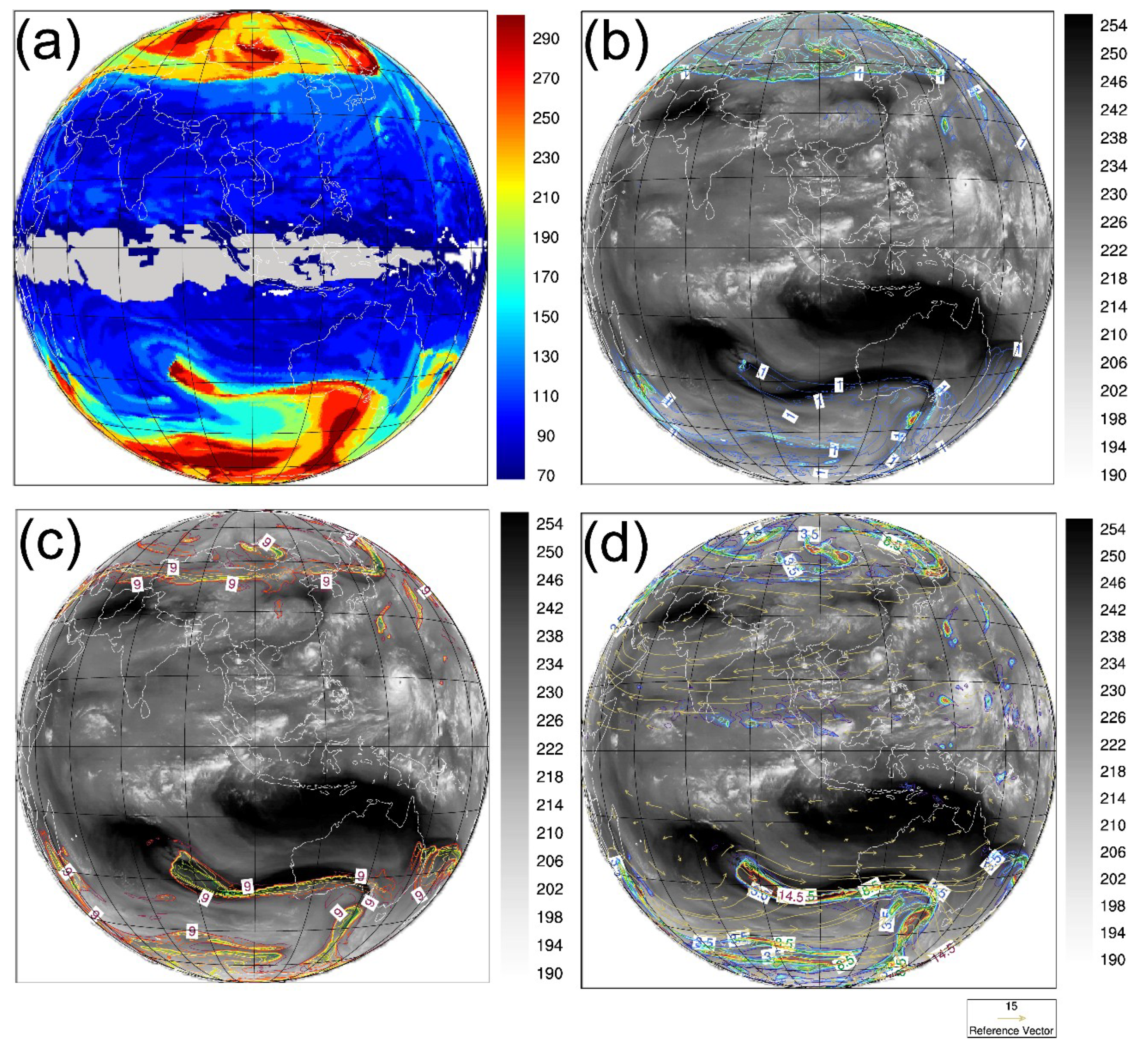
Figure 2.
Flowchart of the Fengyun-4A dynamical tropopause pressure retrieval based on statistical methods.
Figure 2.
Flowchart of the Fengyun-4A dynamical tropopause pressure retrieval based on statistical methods.

Figure 3.
Comparisons of geographical distributions of the dynamical tropopause pressure on 0600 UTC 11 September 2018 retrieved based on the (a) linear regression; (b) gradient boosted decision trees (GBDT) method; (c) K-nearest neighbor (KNN) method; and (d) random forest (RF) method, respectively.
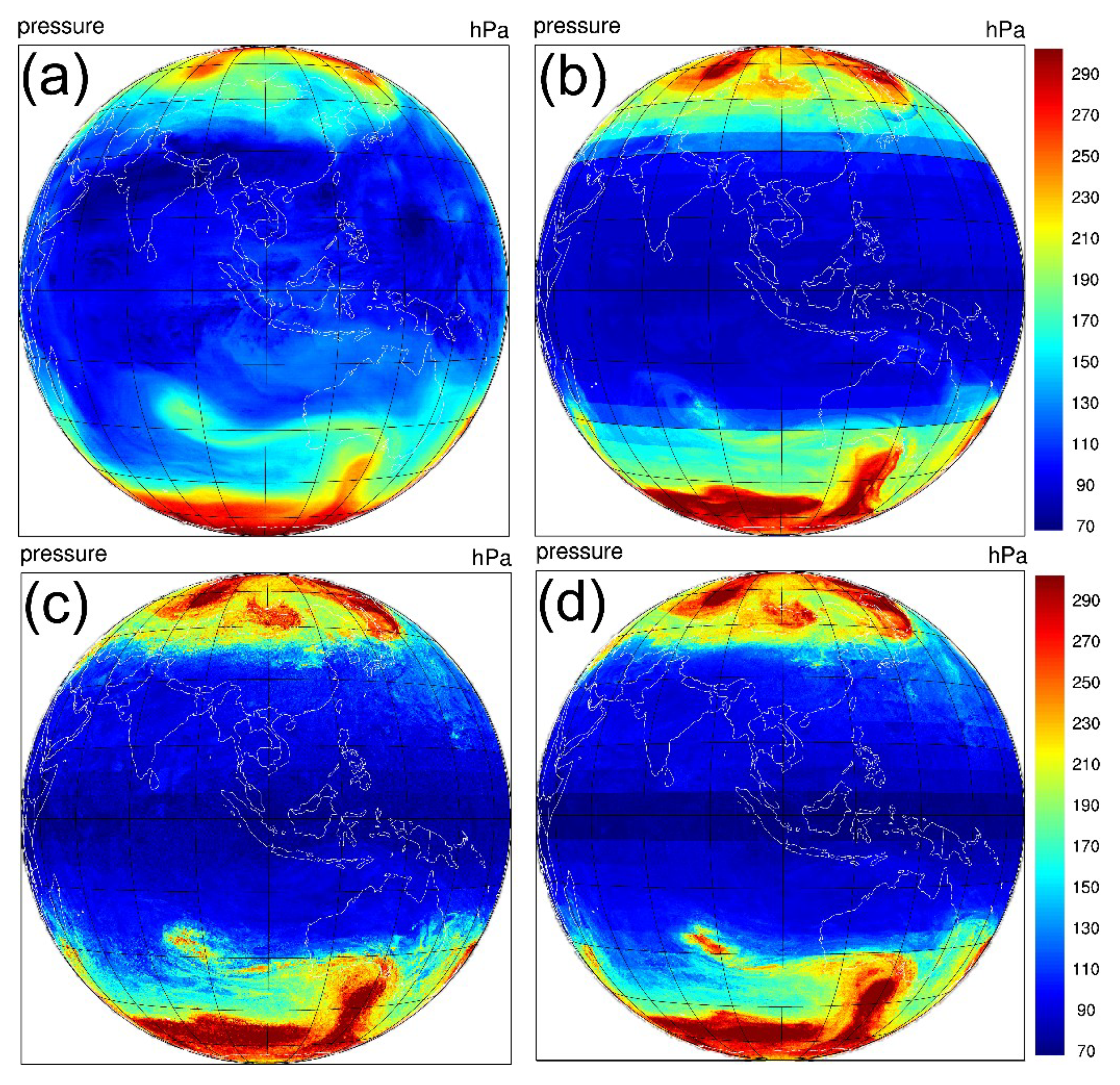
Figure 4.
Comparisons of the mean bias errors (MBE, blue line), root mean square errors (RMSE, black line), standard deviations (σ, green line) and correlation coefficients (R, red line) between the retrievals for the dynamical tropopause pressure on 0600 UTC 11 September 2018 obtained by four statistical retrieval models.
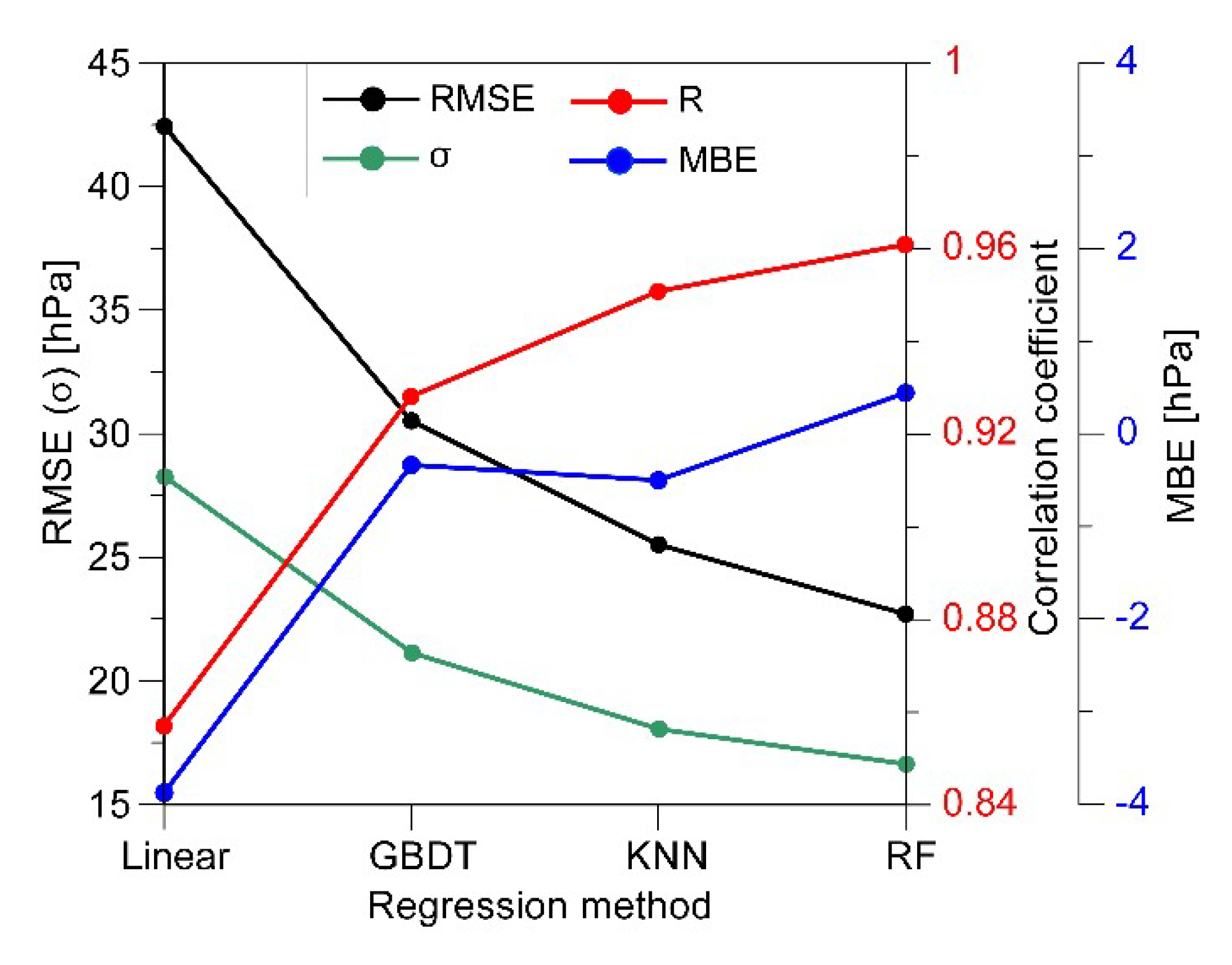
Figure 5.
A yearly distributions of the (a) mean bias error (MBE, blue dots); (b) root mean square error (RMSE, black dots); (c) standard deviation (σ, green dots); and (d) correlation coefficient (R, red dots) between the GEOS-5/MERRA-2 and Fengyun-4A derived tropopause pressure in 2018.
Figure 5.
A yearly distributions of the (a) mean bias error (MBE, blue dots); (b) root mean square error (RMSE, black dots); (c) standard deviation (σ, green dots); and (d) correlation coefficient (R, red dots) between the GEOS-5/MERRA-2 and Fengyun-4A derived tropopause pressure in 2018.
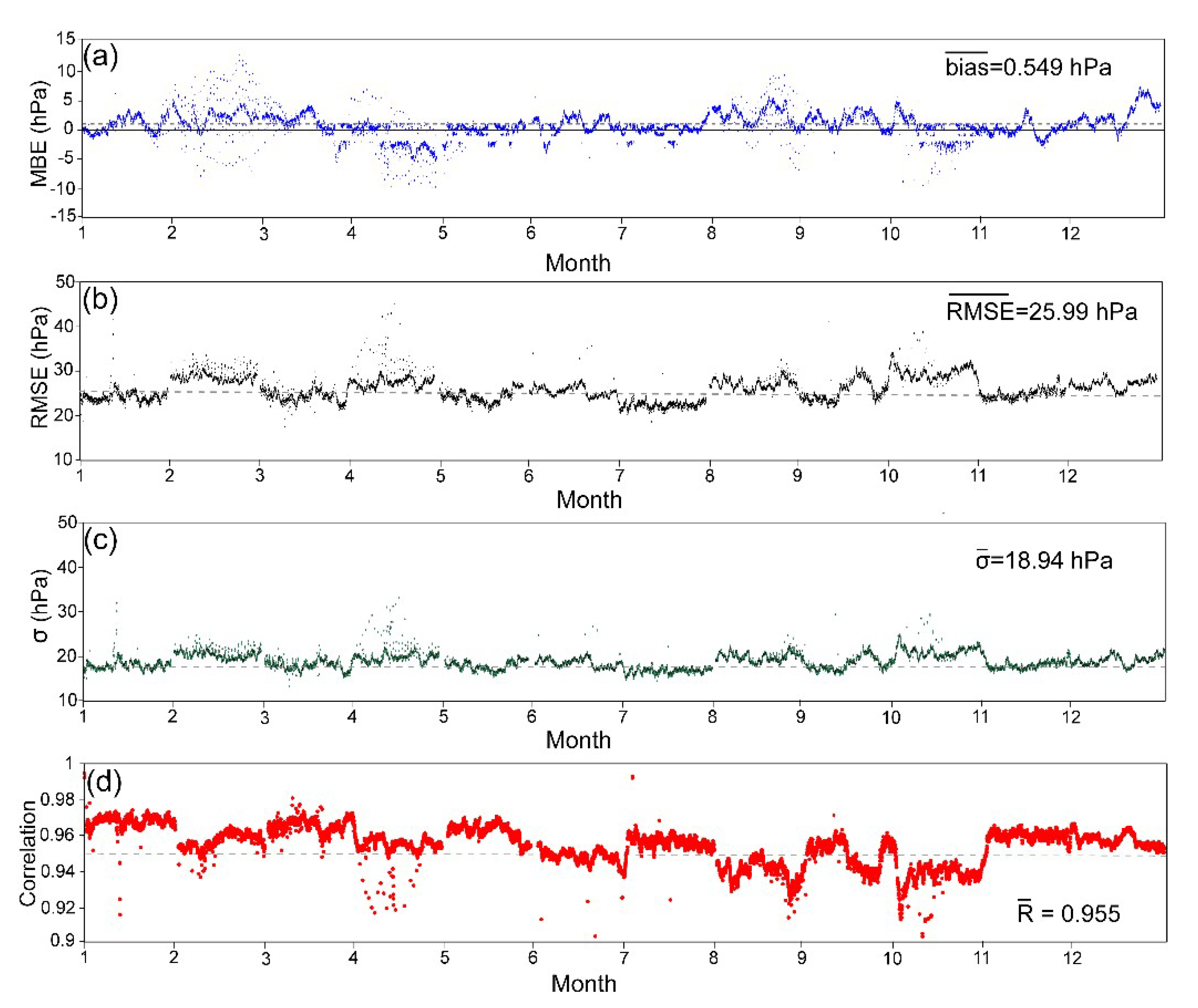
Figure 6.
A yearly distributions of the (a) mean bias error (MBE, blue dots); (b) root mean square error (RMSE, black dots); (c) standard deviation (σ, green dots); and (d) correlation coefficient (R, red dots) between the ERA-Interim and Fengyun-4A derived tropopause pressure in 2018.
Figure 6.
A yearly distributions of the (a) mean bias error (MBE, blue dots); (b) root mean square error (RMSE, black dots); (c) standard deviation (σ, green dots); and (d) correlation coefficient (R, red dots) between the ERA-Interim and Fengyun-4A derived tropopause pressure in 2018.

Figure 7.
The annual and zonal mean (80°S–80°N, 25°–180°E) tropopause-relative profiles of potential vorticity in the ERA-Interim (black dashed line), GEOS-5/MERRA-2 (black solid line) and Fengyun-4A (red solid line) derived tropopause coordinates.
Figure 7.
The annual and zonal mean (80°S–80°N, 25°–180°E) tropopause-relative profiles of potential vorticity in the ERA-Interim (black dashed line), GEOS-5/MERRA-2 (black solid line) and Fengyun-4A (red solid line) derived tropopause coordinates.
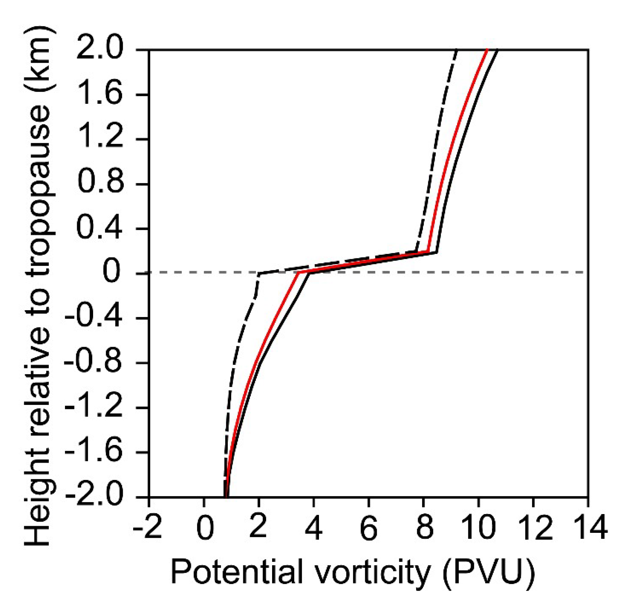
Figure 8.
The annual zonal mean (80°S–80°N, 25°–180°E) tropopause-relative profiles of (a) potential temperature (K), (b) specific ratio of water vapor (g kg−1), and (c) wind speed (m s−1) in the ERA-Interim (black dashed line), GEOS-5/MERRA-2 (black solid line), and Fengyun-4A (red solid line) derived tropopause coordinates.
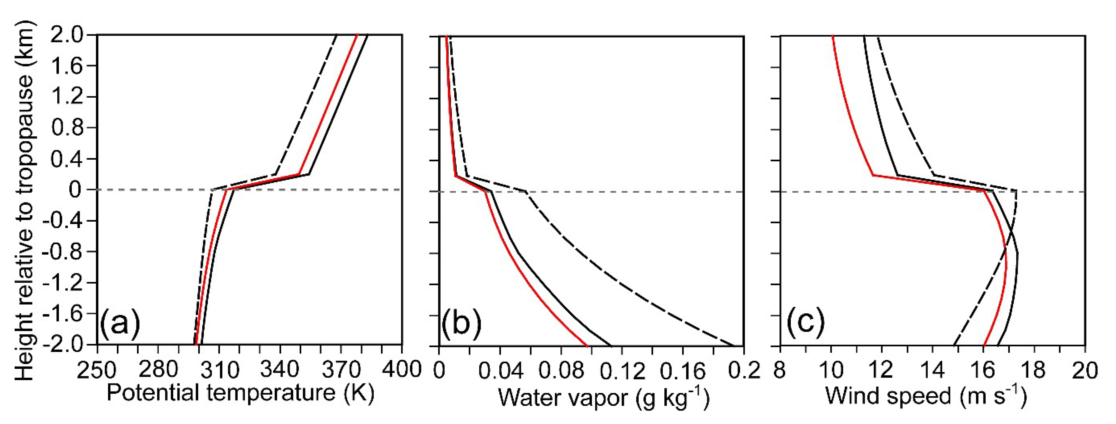
Figure 9.
Geographical dynamical tropopause pressure distributions for DJF (DJF: December, January, February; left panels) and JJA (JJA: June, July, August; right panels) derived by (a,b) ERA-Interim reanalysis and (c,d) Fengyun-4A satellite observations.
Figure 9.
Geographical dynamical tropopause pressure distributions for DJF (DJF: December, January, February; left panels) and JJA (JJA: June, July, August; right panels) derived by (a,b) ERA-Interim reanalysis and (c,d) Fengyun-4A satellite observations.
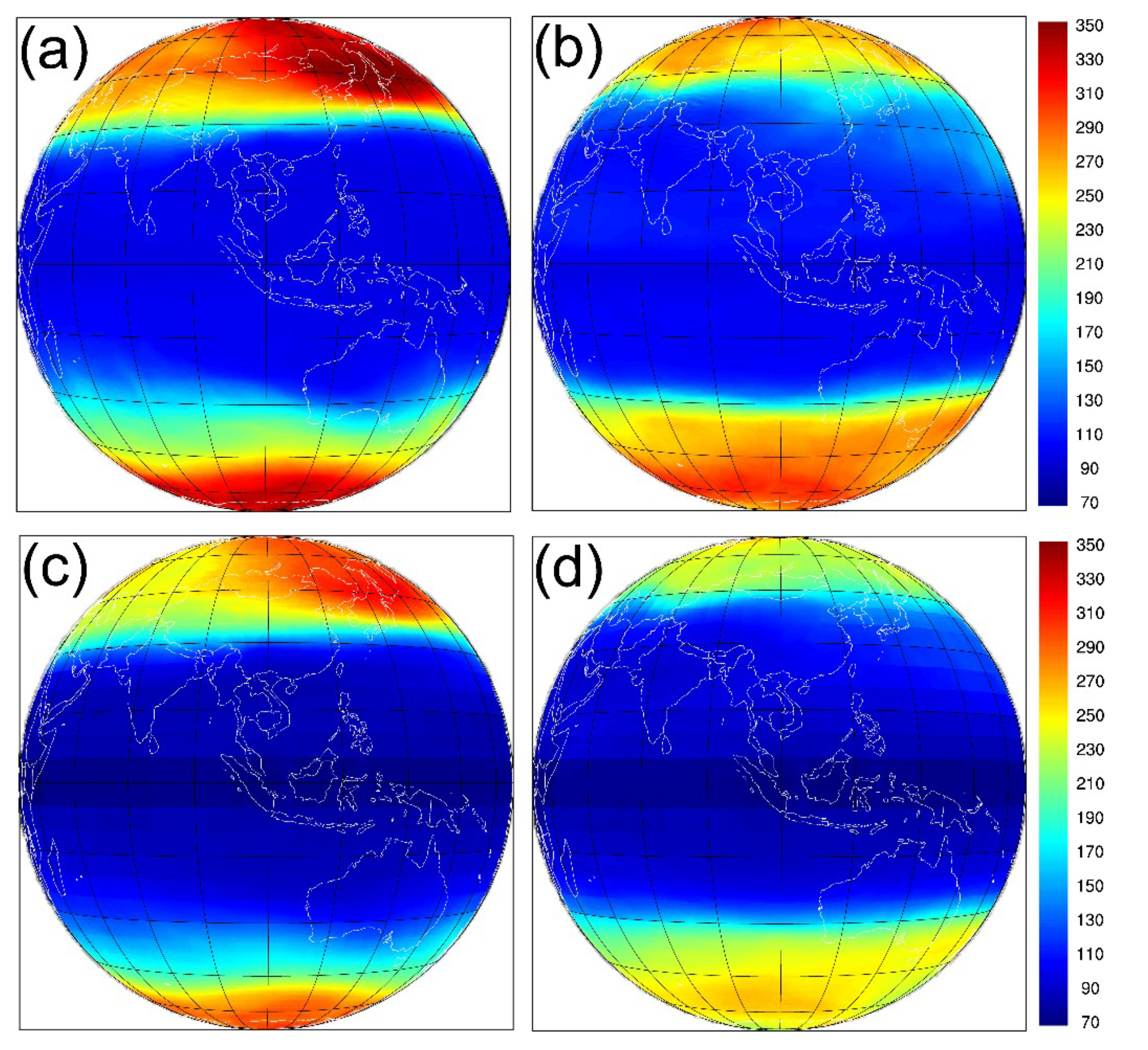
Figure 10.
Contribution scores of the predictors in the RF-based Fengyun-4A dynamical tropopause pressure retrieval model.
Figure 10.
Contribution scores of the predictors in the RF-based Fengyun-4A dynamical tropopause pressure retrieval model.


Table 1.
Physical bases of the predictors used in dynamical tropopause retrieval models.
| Variables. | Physical Bases |
|---|---|
| TBB6.25 μm | Upper-tropospheric water vapor content, upper-level jets, turbulence |
| AWV6.25 μm | Upper-tropospheric water vapor content, upper-tropospheric potential vorticity |
| TBB7.1 μm | Mid-tropospheric water vapor content, upper-level jets, turbulence |
| AWV7.1 μm | Mid-tropospheric water vapor content, mid-tropospheric potential vorticity |
| TBB10.8 μm | Convection, cloud-top height, columnar water vapor content |
| TBB12.0 μm | Convection, cloud-top height, columnar water vapor content |
Table 2.
Statistical parameters (MBE: mean bias error; RMSE: root mean square error; σ: standard deviation; R: correlation coefficient) of tropopause pressure (in hPa) retrieved by different regression schemes in two latitudinal zones: low latitudes (0°–30°) and midlatitudes (30°–60°).
Table 2.
Statistical parameters (MBE: mean bias error; RMSE: root mean square error; σ: standard deviation; R: correlation coefficient) of tropopause pressure (in hPa) retrieved by different regression schemes in two latitudinal zones: low latitudes (0°–30°) and midlatitudes (30°–60°).
| Latitudinal Zone | 0°–30° | 30°–60° | |||||||
|---|---|---|---|---|---|---|---|---|---|
| Method | MBE (hPa) | RMSE (hPa) | σ (hPa) | R | MBE (hPa) | RMSE (hPa) | σ (hPa) | R | |
| Linear | 11.983 | 27.75 | 17.35 | 0.530 | −25.60 | 49.85 | 32.37 | 0.814 | |
| GBDT | −3.237 | 19.03 | 13.61 | 0.734 | 0.8645 | 39.23 | 24.59 | 0.846 | |
| KNN | −3.031 | 17.73 | 12.69 | 0.762 | 0.705 | 31.86 | 21.41 | 0.895 | |
| RF | −1.784 | 15.65 | 11.77 | 0.838 | 1.942 | 28.22 | 19.74 | 0.919 | |
Table 3.
Description of experiment design.
| Experiment | Description |
|---|---|
| CNTL | Retrieval model is built based on predictors of time, latitude, longitude, TBBs of 10.8 μm, 12 μm, 6.25 μm, 7.1 μm, and the AWVs of 6.25 μm and 7.1 μm |
| NTIM | Remove time |
| NLAT | Remove latitude |
| NCLD | Remove TBBs of 10.8 μm and 12 μm |
| NHWV | Remove TBB and AWV of 6.25 μm |
| NMWV | Remove TBB and AWV of 7.1 μm |
Table 4.
Root mean square errors and correlation coefficients between GEOS-5/MERRA-2 and Fengyun-4A derived dynamical tropopause pressure on 0600 UTC 11 September 2018 obtained by six experiment schemes listed in Table 2 (sample number: N = 67,796).
Table 4.
Root mean square errors and correlation coefficients between GEOS-5/MERRA-2 and Fengyun-4A derived dynamical tropopause pressure on 0600 UTC 11 September 2018 obtained by six experiment schemes listed in Table 2 (sample number: N = 67,796).
| Statistics | CNTL | NTIM | NLAT | NCLD | NHWV | NMWV |
|---|---|---|---|---|---|---|
| RMSE (hPa) | 22.7 | 26.19 | 34.12 | 30.94 | 35.74 | 32.81 |
| Correlation | 0.96 | 0.94 | 0.9077 | 0.9229 | 0.8947 | 0.9123 |
© 2020 by the authors. Licensee MDPI, Basel, Switzerland. This article is an open access article distributed under the terms and conditions of the Creative Commons Attribution (CC BY) license (http://creativecommons.org/licenses/by/4.0/).
Share and Cite
MDPI and ACS Style
Shou, Y.-X.; Lu, F.; Shou, S. High-Resolution Fengyun-4 Satellite Measurements of Dynamical Tropopause Structure and Variability. Remote Sens. 2020, 12, 1600. https://doi.org/10.3390/rs12101600
AMA Style
Shou Y-X, Lu F, Shou S. High-Resolution Fengyun-4 Satellite Measurements of Dynamical Tropopause Structure and Variability. Remote Sensing. 2020; 12(10):1600. https://doi.org/10.3390/rs12101600
Chicago/Turabian StyleShou, Yi-Xuan, Feng Lu, and Shaowen Shou. 2020. "High-Resolution Fengyun-4 Satellite Measurements of Dynamical Tropopause Structure and Variability" Remote Sensing 12, no. 10: 1600. https://doi.org/10.3390/rs12101600
Note that from the first issue of 2016, this journal uses article numbers instead of page numbers. See further details here.