Modelling Distributions of Rove Beetles in Mountainous Areas Using Remote Sensing Data

Abstract

Mountain ecosystems are biodiversity hotspots that are increasingly threatened by climate and land use/land cover changes. Long-term biodiversity monitoring programs provide unique insights into resulting adverse impacts on plant and animal species distribution. Species distribution models (SDMs) in combination with satellite remote sensing (SRS) data offer the opportunity to analyze shifts of species distributions in response to these changes in a spatially explicit way. Here, we predicted the presence probability of three different rove beetles in a mountainous protected area (Gran Paradiso National Park, GPNP) using environmental variables derived from Landsat and Aster Global Digital Elevation Model data and an ensemble modelling approach based on five different model algorithms (maximum entropy, random forest, generalized boosting models, generalized additive models, and generalized linear models). The objectives of the study were (1) to evaluate the potential of SRS data for predicting the presence of species dependent on local-scale environmental parameters at two different time periods, (2) to analyze shifts in species distributions between the years, and (3) to identify the most important species-specific SRS predictor variables. All ensemble models showed area under curve (AUC) of the receiver operating characteristics values above 0.7 and true skills statistics (TSS) values above 0.4, highlighting the great potential of SRS data. While only a small proportion of the total area was predicted as highly suitable for each species, our results suggest an increase of suitable habitat over time for the species Platydracus stercorarius and Ocypus ophthalmicus, and an opposite trend for Dinothenarus fossor. Vegetation cover was the most important predictor variable in the majority of the SDMs across all three study species. To better account for intra- and inter-annual variability of population dynamics as well as environmental conditions, a continuation of the monitoring program in GPNP as well as the employment of SRS with higher spatial and temporal resolution is recommended.

1. Introduction

Mountain ecosystems are biodiversity hotspots with higher species richness and levels of endemism than adjacent lowlands as a result of steep environmental gradients over short distances that lead to topographic, geologic, and climatic heterogeneity [1,2]. Such physiographic complexity creates a mosaic of habitats and, hence, a multitude of ecological niches. Furthermore, spatial isolation of mountain ridges by environmentally very different lower elevations enhances the segregation of populations and, potentially, speciation. Mountains also play a key role in providing ecosystem services [3], e.g., they supply half of the global human population with fresh water [4]. At the same time, mountain regions are especially sensitive to the impacts of a changing climate as seen by the shrinking of glaciers, changes in water provisioning, and the increase of extreme events such as avalanches and landslides [5].

To understand the impacts of these changes on plant and animal species distributions, long-term biodiversity monitoring initiatives are needed to develop adapted conservation measures [6]. While data collection is a time-consuming endeavor by itself, accessibility is an additional major challenge in mountains. However, such in situ data are indispensable for predicting species occurrence probability at larger scale using, e.g., species distribution models (SDMs, see [7] for detailed information). SDMs based on species data stemming from standardized biodiversity monitoring schemes instead of opportunistic observations have been shown to provide higher model accuracy even with a lower sample size [8]. However, not only reliable species presence data, but also geospatial information on ecologically relevant environmental factors is needed. Since ecological niches in mountains are largely influenced by micro-topography [9], geospatial data created by employing spatial interpolation techniques (e.g., for climatic data, [10]) is often not capable of capturing such small-scale differences and heterogeneity.

Besides climatic data, which governs species distribution at coarse resolution, land use/land cover (LULC) is a main determinant of species presence/absence at finer resolutions [11]. However, existing LULC maps are often not thematically detailed enough and the temporal resolution may be inadequate to improve predictions of species distributions [12,13,14]. In this study, we therefore used satellite remote sensing (SRS) data offering great potential to mirror spatially explicit habitat characteristics for use in SDMs [15]. Furthermore, SRS data is often the only consistent source of information on environmental gradients in space and time allowing also retrospective analyses. However, the use of SRS data in mountain regions is challenging, e.g., due to high and persistent cloud and snow cover, strong illumination effects, and often short vegetation periods (see [16] for more detailed information and possible ways forward). Therefore, only a limited number of studies so far has employed satellite-derived parameters for SDMs in mountainous regions (but see [17,18]).

The use of SRS data for assessing taxonomic, structural, and functional biodiversity research has generally been increasing in recent years [19], driven by a free and open access data policy together with rapid sensor developments offering increasing spatial, temporal, and spectral resolution of satellite imagery [20]. Most importantly, the recently available high-resolution and high-frequent data of the Sentinel-2 mission allows a much more detailed characterization of vegetation phenology [21], improved mapping of fine-scaled habitat types [22], and better assessment of nature conservation status [23]. However, despite these promising developments, studies employing SRS data for analyzing temporal trends in biodiversity face a number of limitations in data availability. Due to the availability of a consistent and cross-calibrated multi-decadal data record and a long-term systematic data acquisition strategy, Landsat satellite imagery is a unique monitoring tool for biodiversity assessments over time at a high spatial scale [24,25].

The objective of this study was to evaluate the potential of Landsat data for predicting the presence of different rove beetles (order Coleoptera, family Staphylinidae) in the Gran Paradiso National Park (GPNP), a mountainous protected area in northwestern Italy. Specifically, we analyzed species data from two different field campaigns (2006–2007 and 2012–2013) to track changes in time and to test model stability. Staphylinids are key organisms in various terrestrial ecosystems and, together with carabid beetles, ants, and spiders, constitute the vast majority of epigeic mesoarthropods (i.e., invertebrate animals that live on the soil surface) [26]. They are abundant, taxonomically and trophically diverse, occupy a variety of ecological niches, and can be easily sampled; all these characteristics make them an attractive taxon for use as bioindicators [27,28]. Moreover, many rove beetle species respond to and depend on local-scale environmental parameters and resources [27,28,29], representing an important challenge for the application of SRS data. In the present study, we focused on three species with fairly different habitat requirements. To collate a well-constructed set of predictor variables relevant to the biology of the species [30], we derived a set of selected topographic and environmental features addressing the peculiarities of the mountainous region studied. We used a state-of-the-art ensemble modelling framework (i.e., an approach that integrated multiple individual model predictions to obtain a final, more accurate one; [31]) that combined two regression-based methods (generalized linear models (GLM) and generalized additive models (GAM) [32,33]) and three machine-learning methods (random forest (RF), generalized boosting models (GBM), and maximum entropy (MAXENT) [34,35,36]) by means of weighted average, an approach suggested to have higher accuracy than single-algorithm models and to perform best among consensus methods [37]. In particular, we addressed the following questions:

• How well can habitat suitability be modelled based on SRS data for rove beetles in mountainous ecosystems?
• How and why do SRS-based model predictions differ among years?
• What are the most important SRS predictors? How do they differ among species?

2. Materials and Methods

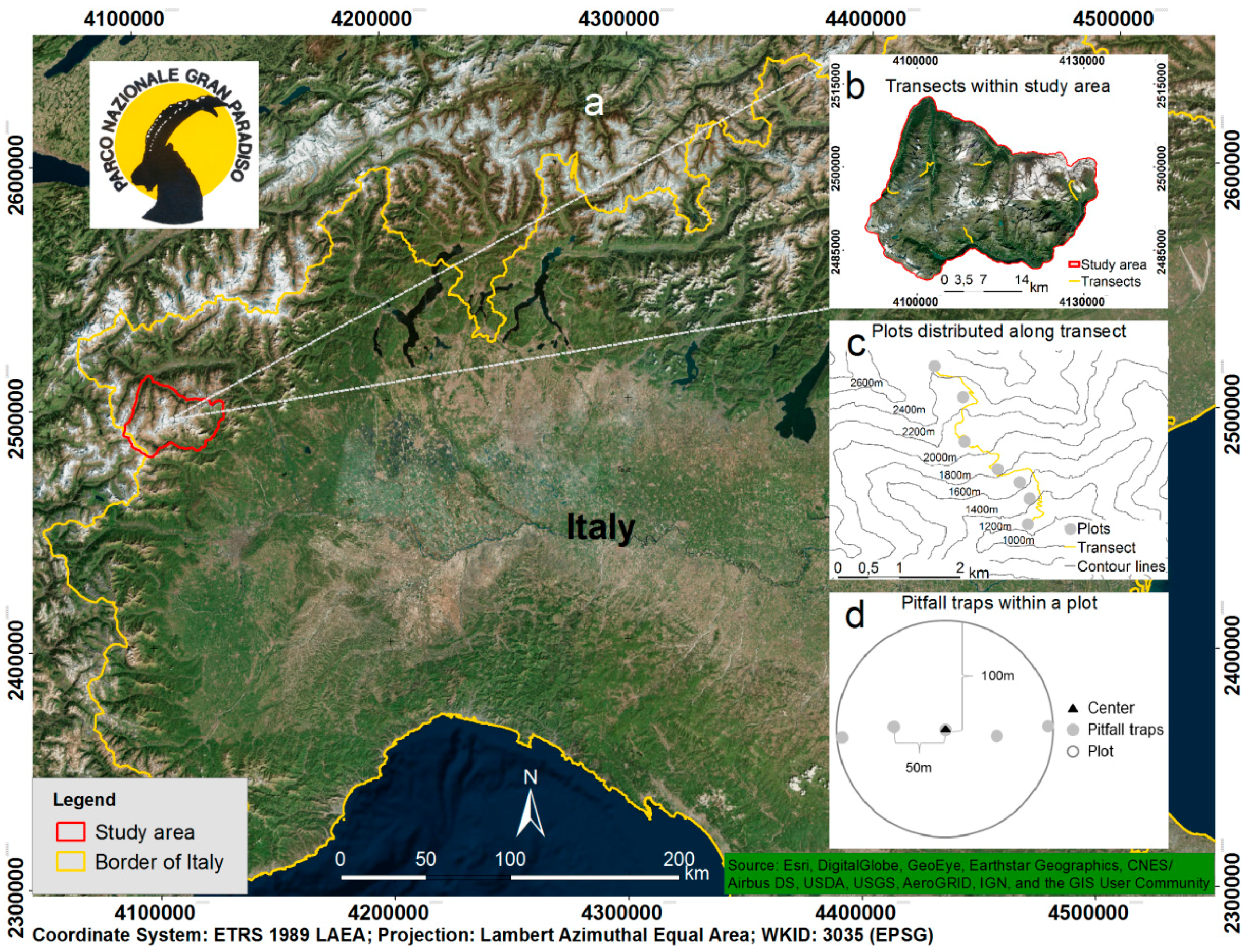
2.1. Study Area

The study region encompassed the territory of the Gran Paradiso National Park (GPNP, total area of 847.4 km²) located in northwestern Italy (Figure 1a). GPNP is the oldest national park in Italy that gained official conservation status in 1922 and provides habitat for the threatened alpine ibex (Capra ibex). The park is part of the Long-Term Ecological Research (LTER, site code: LTER_EU_IT_109) and of the NATURA 2000 (site code: IT1201000) networks and has been subject to intensive long-term monitoring efforts and research [38].

GPNP is characterized by complex topography with elevation ranging from 670 to 4061 m above sea level (a.s.l.) including different altitudinal vegetation belts (montane, subalpine, alpine, and nival) [39]. Woodlands (20.2% of the territory) are dominated by larch (Larix decidua) and Norway spruce (Picea abies) while species-rich alpine grasslands and pastures (17% of the territory) can be found above the treeline. About 60% of the territory is covered with sparse or no vegetation, bare rocks, or glaciers [38,40]. The climate is alpine-continental, characterized by low annual mean temperatures (ca. 5 °C), high seasonal differences, and a general paucity of precipitation (990 mm/year on average). However, remarkable dissimilarities can be observed among different valleys due to variations in altitude, slope, and aspect. Snow cover is usually present from November–December to March–April [41,42].

2.2. Sampling Design for Biodiversity Data and Species Characteristics

Species occurrence data for this study were collected in the context of the long-term monitoring project Monitoring of Animal Biodiversity in Mountain Ecosystems, which is an initiative of the GPNP and the first attempt to develop a protocol for long-term monitoring of multiple taxa in the Italian Alps [39]. The main purpose of this long-term monitoring initiative is to collect information on changes in community composition for multiple taxa [39] to allow analyzing biodiversity changes in time and along elevational gradients. The first monitoring campaign started in 2006–2007 and campaigns (carried out over a two-year period) will be continued every six years.

The monitoring scheme encompasses five representative altitudinal transects to cover three vegetation belts (high montane, subalpine, alpine; elevational range 1200–2600 m a.s.l.; Figure 1b). Sampling units are plots (circular areas with 100 m radius, between five and seven per transect, resulting in a total of 30 plots for GPNP, Figure 1c), which are separated by an altitudinal difference of approximately 200 m to allow for data independence. Pitfall traps in each plot were set up along one diameter of the plot with a distance of 50 m from each other (Figure 1d). Species presence/absence data were collected using pitfall traps (plastic cups, diameter of 7 cm, filled with ca. 10 cc of white vinegar and some drops of detergent to break surface tension). The traps were emptied and refilled every two weeks from May to September. Sampled adult specimens were identified at the species level by taxonomic experts who registered presence/absence for each taxon.

Here, we focus on rove beetles (Coleoptera: Staphylinidae) using data from the two monitoring campaigns in 2006–2007 and 2012–2013. Rove beetles have been previously shown to be sensitive to ecosystem modification and anthropogenic impacts [43,44]. Pitfall traps (when being active for a whole season) can be considered suitable for obtaining estimates of presence/absence as well as relative population density and for quantifying population fluctuations in epigeal Coleoptera and allow a standardized and repeatable sampling through space and time [45,46]. Among the 178 species present in the database, we here selected three (Dinothenarus fossor, Platydracus stercorarius, and Ocypus ophthalmicus) for which a sufficiently high number of sampling locations was available, and which were not highly localized within our study area. We chose rather common species for which taxonomy, general habitat requirements, and ecological traits are reasonably well known [27]. From those, we focused on species with taxonomic proximity (same subfamily and tribe, Staphylininae Staphylinini), but characterized by quite different ecological and functional specialization, in particular in terms of macro- and micro-habitat affinity and altitudinal range. For detailed species characteristics see Box 1 and description in Section S1 in the supplementary.

Box 1. Characteristics of the Staphylinidae species used for species distribution modelling according to Tagliapietra and Zanetti [47] and Zanetti et al. [48]. Source of photographs: Iconographia Coleopterorum Poloniae by Lech Borowiec (http://baza.biomap.pl).

	Dinothenarus fossor	Platydracus stercorarius	Ocypus ophthalmicus
Size	15–20 mm	12–15 mm	15–23 mm
Macro-habitat	Sylvicolous (mainly)	Eurytopic	Often in open areas (eurytopic)
Micro-habitat	Phytodetriticolous (mainly)	Saprophilous (often close to dung)	Phytodetriticolous
Nutrition	Predator (mainly myrmecophagous)	Generalist predator (other insects)	Generalist predator (other insects, larvae, nematodes, snails)
Micro-climate	Xerophilus	NA	Xerophilus, heliophilous
Altitude	Montane (mainly)	Lowland to montane	Lowland to subalpine-alpine
Chorotype	Central European	Turano-European	Palearctic

2.3. Species Presence/Pseudo-Absence Data for Model Training

To train the SDMs, we used the environmental conditions at the trap locations in which individuals of each target species were captured (true presence data), separately for each species. The number of traps and plots in which individuals of each species were captured varied among species and years (

Table 1. Number of traps, plots, and transects in which individuals of each species were captured, located in areas free of cloud and snow cover in the analyzed SRS data. Number of plots (used as presence data) used for modelling and the correspondent time periods are highlighted in bold.

	Dinothenarus fossor						Platydracus stercorarius						Ocypus ophthalmicus
Year(s)	2006	2007	2012	2013	2006/2007	2012/2013	2006	2007	2012	2013	2006/2007	2012/2013	2006	2007	2012	2013	2006/2007	2012/2013
Traps	42	36	55	49	52	66	14	12	25	35	22	45	19	15	16	16	27	26
Plots	15	15	18	17	17	19	9	10	14	16	12	18	11	10	9	10	14	12
Tran-sects	4	5	4	4	5	4	4	5	5	5	5	5	5	5	4	5	5	5

). Furthermore, a few samples were excluded from the analysis as located in areas covered by clouds and snow in the analyzed SRS data. For all species and both monitoring campaigns, we pooled the data collected in 2006–2007 and 2012–2013, respectively, thereby increasing the number of traps and plots in which individuals were captured (Table 1). The use of data from consecutive years is a common approach in species distribution modelling to account for inter-annual differences in species abundance and occurrence [49]. We initially used all traps where the study species were captured as presence points for fitting the models, but, due to the close proximity of traps within plots, then decided to model each species on plot-pooled data by subsampling only one trap per plot as presence point. For each plot, we selected the trap with the highest number of captured individuals per species, thus ensuring that the site was recurrently frequented by the study species. Subsampling is an effective way of removing pseudo-replicates (i.e., spatially correlated observations) in the dataset. Although this approach further reduced the number of presences available for modelling, previous studies [50,51] showed that accurate SDMs can be fitted on very small numbers of training records.

Due to the limited size of our dataset, we decided not to use traps without captured individuals as absence information but to generate pseudo-absence data. Pseudo-absences are commonly used in distribution modelling [52], and they should not be interpreted as sites at which the species was truly absent, but rather as a sample of the environmental variation in the study area [53,54]. Moreover, this approach allowed us to use the true absences as an independent dataset for subsequent model evaluation (see Section 2.7). Specifically, we created 500 stratified random point locations as pseudo-absence data, which were allocated according to the sampling design in terms of trap density at specific altitudinal ranges (Figure 1c; e.g., 6.7% of the traps were located at 1300 m a.s.l. thus 33 out of 500 random points were assigned to the range 1300 ± 50 m). Additional constraints for the locations of these stratified random points were a minimum distance of 30 m between points to match the spatial scale of the analyzed satellite remote sensing data (see Section 2.4.) and the non-existence of points within a buffer area with 500 m diameter around trap locations (for detailed information see Figure S1). This buffer acknowledged the necessity to use reasonable pseudo-absences that are adequately environmentally distant from the presence data (but not outside the area of interest) in order to avoid inflation of AUC (area under curve of the receiver operating characteristics) values [55]. Areas covered by clouds and snow were excluded for allocation of pseudo-absence data.

2.4. Satellite Remote Sensing Data

We used multispectral Landsat surface reflectance data provided by the Earth Resources Observation and Science Centre Processing Architecture [56]. Landsat imagery has proven suitable to derive geospatial information on environmental characteristics that affect species distributions in multiple studies [18,57] and has been used to model changes in biodiversity between different time periods [58]. Two Landsat images acquired on 22 September 2006 (Landsat 5-TM) and 9 September 2013 (Landsat 8-OLI) that were consistent with the time period of in situ species data sampling (between May and September) were downloaded. These images were selected to minimize overall cloud cover over the study area (41.6% in 2006 and 25.3% in 2013) and differences between acquisition dates. We topographically corrected the images and calculated the tasseled cap transformation to derive “brightness”, “greenness”, and “wetness” using sensor-specific coefficients [59,60]. Additionally, we derived the Normalized Difference Vegetation Index (NDVI, [61]) and downloaded the NDVI-based land surface temperature (LST) for each acquisition date [62].

In order to represent altitudinal and topographic gradients, the ASTER Global Digital Elevation Model (GDEM, cell size: 30 × 30 m, [63]) was aligned to match pixel locations of the Landsat imagery. While the use of altitude information has been subject to debate in ecology in general [1] and in species distribution modelling in particular [9,64], we here used altitude as a proxy for climatic parameters since spatially explicit estimates of climate were not available at sufficiently high spatial resolution. In addition, based on the ASTER GDEM, the Terrain Ruggedness Index (TRI, based on 8 adjacent cells within a quadratic array around the center cell [65]), sine of aspect (eastness), cosine of aspect (northness), and slope were calculated. Areas covered by clouds, cloud shadows, and snow were masked out (Figure S2). To avoid collinearity of explanatory variables in the subsequent analyses, a threshold of |r| > 0.7 was used to exclude variables [66]. As a result, NDVI was not used in the modelling framework due to its strong correlation with altitude. Likewise, brightness and land surface temperature were also excluded as they were highly correlated with northness and wetness (Figure S3). An overview of the SRS variables used and their ecological relevance is given in

Table 2. Characteristics of noncorrelated SRS-based variables used in species distribution modelling. Abbreviations: TCT, tasseled cap transformation. References indicate studies highlighting the ecological relevance of the considered variables.

Variable	Ecological Relevance	References	Source
Altitude	Directly correlated with temperature, of particular importance in mountain ecosystems	[9,18,67]	ASTER GDEM
Eastness/Northness	Gradients represent differences in the aspect affecting irradiation and precipitation (e.g. an orientation towards east favours heating up in the morning while west-facing ensure higher temperatures in the afternoon)	[68,69]	ASTER GDEM
Slope	Terrain steepness reflects gradients in humidity, thickness of soil layer and transport dynamics of matter	[18]	ASTER GDEM
Terrain Ruggedness Index	Represents elevational differences among neighbouring grid cells (high values relate to large topographic heterogeneity and impenetrable terrain)	[65,70]	ASTER GDEM
Greenness (TCT)	Responds to photosynthetic capacity, vegetation cover and primary productivity (sensitive to topography)	[71,72]	Landsat imagery
Wetness (TCT)	Responds to soil/canopy moisture and standing water, being often highest in young forest stands (not sensitive to topography)	[73,74]	Landsat imagery

.

2.5. Ensemble Modelling and Model Parametrization

Since the choice of model algorithm is a major component of prediction uncertainty in SDMs [37,75], several algorithms were employed and combined in order to estimate and account for prediction uncertainty (ensemble modelling, [31]). We used five modelling methods that are representative for different classes of model algorithms, namely generalized linear models and generalized additive models (GLM and GAM, regression-based methods, [32,33]), random forest, generalized boosting models, and maximum entropy (RF, GBM, and MAXENT; machine-learning methods; [34,35,36]) as implemented in the biomod2 package version 3.3 [76] using R version 3.6.0 [77]. To account for the within-algorithm model variation when different sets of data were used for model fitting, we computed distribution models for each species using 50 repetitions where 70% of the data were used for model training and 30% for model testing. To avoid spatial sorting bias in the cross-validation procedure [78], we used a spatially stratified approach to split the training and the testing data sets, to prevent selecting testing-presence sites close to training-presence sites. Specifically, the full dataset was divided into 50 clusters (one for each model repetition), using k-means clustering based on the spatial coordinates of presence/pseudo-absence points. For each model run, 30% of the points closest to the center coordinates of the respective cluster were used as testing dataset and the remaining as training dataset. Model outputs were scaled between 0 and 1000 to ensure comparability of model predictions across the different model algorithms. A binomial link function was used to fit GLMs, allowing linear and quadratic terms as well as linear interactions of the explanatory variables. To simplify the full model (i.e., to reduce the number of environmental predictors by removing less important ones), a stepwise backward selection was applied to select final models, based on the Bayesian Information Criterion (BIC) [79]. GAMs were also fitted with a binomial link function, including all seven explanatory variables and using the algorithm as implemented in the mgcv package [80]. The basis dimension of the smooth functions was set to k = 4 to avoid overfitting. For MAXENT, the maximum number of iterations was set to 500 and the ‘Auto feature’ settings were used while excluding threshold and hinge features to avoid over-parameterization [81]. The regularization parameter β was set to 0.002 to optimize model performance [82]. For RF models we used 500 trees, following previous studies [75], while for GBMs we used the default settings (number of trees = 100, interaction depth parameter = 1, learning rate = 0.1, and subsampling fraction = 0.5) suggested by the gbm package [83]. The AUC was used as evaluation criteria to generate the ensemble predictions from the five different algorithms (see biomod2 documentation for further details). To obtain a relevant combination of several unbiased (i.e., with fair accuracy) models, all individual models with an AUC value <0.7 were discarded, and the ensemble models were constructed for each species and time period by computing the weighted average of all remaining model predictions [52]. The weights were based on the AUC scores of each model, so that better performing models had a higher influence in the final ensemble. This technique has been shown to be one of the best performing consensus methods [37] and is widely used in ensemble applications [52]. To assess shifts in suitable habitat between the two time periods, we defined five classes of habitat suitability based on the presence probability scores extracted from the SDM maps. The five classes were defined by the following thresholds of presence probability scores: 0–200, >200–400, >400–600, >600–800, and >800–1000, ordered from low to high habitat suitability. To compare changes over time, we calculated the percentage of area in each class for the common area not masked by cloud, shadow, and snow coverage in either of the two time periods. Moreover, we calculated Spearman rank correlation coefficients between the SDMs, to assess the correlation of species distributions between time periods and across different species.

2.6. Assessing Variable Importance of SRS Data

Variable importance was assessed by comparing the model prediction derived from the original dataset and predictions derived from permuted datasets [76,84]. Permuted datasets were created by randomizing one environmental variable resulting in one dataset for each predictor variable. The predictions of occurrence probabilities resulting from permuted datasets and the original dataset were compared by calculating the Pearson correlation coefficient; a small correlation coefficient thus indicated high importance of the permuted variable. This procedure was repeated three times for each model run, and mean correlation values for each predictor variable were derived across the 50 model repetitions. Values of variable importance were finally calculated by subtracting the correlation coefficient from 1. To ensure comparability between different model algorithms, the relative variable importance was calculated for every variable per algorithm. To understand the effect of single variables on the SDM predictions, response curves showing the sensibility of the model to each variable were plotted for all variables in the ensemble models [76].

2.7. Model Evaluation

We used a cross-validation procedure to assess model performance and calculated two evaluation metrics commonly used in species distribution modelling, AUC and the true skills statistics (TSS) [54]. AUC values for SDMs indicate how well the model discriminated between species presence and absence/pseudo-absence data [85]. According to Swets [86], models with AUC values below 0.7 are considered as poorly accurate, those with AUC between 0.7 and 0.9 as useful, and those with values above 0.9 as highly accurate. TSS is a threshold-dependent metric, not affected by the size of the validation set nor by species prevalence [54,87]. TSS is calculated as sensitivity (i.e., true positive rate) + specificity (i.e., true negative rate) −1, and therefore ranges from −1 to +1, where values of zero or less indicate a performance no better than random guessing [54]. According to González-Ferreras et al. [88], model accuracy is poor when TSS values are below 0.4, fair when TSS is between 0.4 and 0.6, good when TSS is between 0.6 and 0.8, and excellent for values above 0.8. Mean AUC and TSS scores were calculated based on the 50 model repetitions for all model algorithms and for the ensemble models. In addition to AUC and TSS, we analyzed and compared model predictions at presence locations and at independent true absence data (i.e., traps in which no individuals of each target species were captured) for each species to examine how well derived maps represented in situ data. Finally, as uncertainty maps are an important tool for communicating model reliability in a spatially explicit way [89], we calculated the difference between the 97.5th percentile and the 2.5th percentile of cell values derived from the prediction maps for each species, based on 50 model repetitions.

3. Results

3.1. Model Performance

AUC and TSS values were highly concordant in assessing model performance, and the majority of species prediction models showed satisfactory accuracy levels based on the two evaluation metrics (i.e., AUC > 0.7 and TSS > 0.4,

Table 3. Mean area under curve (AUC) and true skills statistics (TSS) values, with standard deviation (SD), calculated on the 50 model repetitions for the different time periods, species, and model algorithms. AUC values >0.7 and TSS values >0.4 are highlighted in green. Abbreviations: GLM, generalized linear model; GAM, generalized additive model; RF, random forest; GBM, generalized boosting model.

	Dinothenarus fossor
Years	2006/2007				2012/2013
	mean AUC	±SD	mean TSS	±SD	mean AUC	±SD	mean TSS	±SD
GLM	0.549	0.11	0.164	0.17	0.67	0.104	0.354	0.19
GAM	0.717	0.118	0.455	0.185	0.782	0.064	0.557	0.128
MAXENT	0.725	0.083	0.454	0.126	0.801	0.102	0.574	0.191
RF	0.74	0.094	0.5	0.149	0.813	0.085	0.618	0.12
GBM	0.83	0.047	0.588	0.088	0.835	0.064	0.609	0.137
Ensemble	0.845	0.044	0.663	0.076	0.869	0.053	0.666	0.111
	Platydracus stercorarius
Years	2006/2007				2012/2013
	mean AUC	±SD	mean TSS	±SD	mean AUC	±SD	mean TSS	±SD
GLM	0.532	0.073	0.098	0.117	0.529	0.102	0.168	0.169
GAM	0.626	0.124	0.312	0.226	0.625	0.098	0.337	0.117
MAXENT	0.78	0.068	0.605	0.126	0.655	0.055	0.375	0.086
RF	0.638	0.115	0.368	0.161	0.754	0.077	0.505	0.121
GBM	0.664	0.133	0.391	0.221	0.77	0.059	0.542	0.085
Ensemble	0.798	0.058	0.618	0.1	0.788	0.051	0.551	0.095
	Ocypus ophthalmicus
Years	2006/2007				2012/2013
	mean AUC	±SD	mean TSS	±SD	mean AUC	±SD	mean TSS	±SD
GLM	0.685	0.137	0.391	0.267	0.573	0.149	0.186	0.268
GAM	0.8	0.142	0.615	0.26	0.587	0.125	0.22	0.214
MAXENT	0.809	0.148	0.707	0.217	0.709	0.112	0.474	0.141
RF	0.881	0.079	0.754	0.15	0.767	0.102	0.572	0.142
GBM	0.843	0.087	0.7	0.158	0.713	0.14	0.525	0.191
Ensemble	0.893	0.086	0.806	0.145	0.843	0.07	0.672	0.127

), and can thus be categorized as useful [86]. Dinothenarus fossor showed the highest number of well-performing models, probably because of the larger number of presence points in both time periods, compared to the other two species (Table 1). On the contrary, for Platydracus stercorarius, only 5 out of 12 models could be classified as useful, based on the evaluation metrics scores. In the case of Ocypus ophthalmicus, 5 out of the 6 model types built for the time period 2006–2007 performed well, whereas the number decreased to 4 out of 6 for the 2012–2013. Model performance varied significantly across model algorithms, with the machine-learning algorithms GBM, RF, and MAXENT producing the highest AUC and TSS scores. In contrast, GAM and GLM models performed poorly. Moreover, the evaluation metrics values of GLM models showed strong variation for different model repetitions, reflecting the instability of the models. The ensemble models always outperformed all other model types, returning accurate models for all species in both time periods. Contrasting patterns were found when comparing the different time periods 2006–2007 and 2012–2013: For Dinothenarus fossor, we observed higher evaluation metrics scores for the models referring to 2012–2013 across all algorithms. In contrast, for Ocypus ophthalmicus model performance was higher for 2006–2007. No clear pattern was found for Platydracus stercorarius when comparing model accuracy between time periods.

In addition to the cross-validation results, the comparison between modelled presence probabilities at presence locations and at absence records not used for model training revealed that the majority of ensemble models had fair discriminatory power in the prediction of suitable vs. unsuitable habitat. For Dinothenarus fossor, the modelled presence probabilities were significantly higher in the ensemble predictions at presence sites compared to absence sites, in both time periods (Figure 2). However, for the other two species, the ensemble models built for 2006–2007 had higher discriminatory power than those built for 2012–2013.

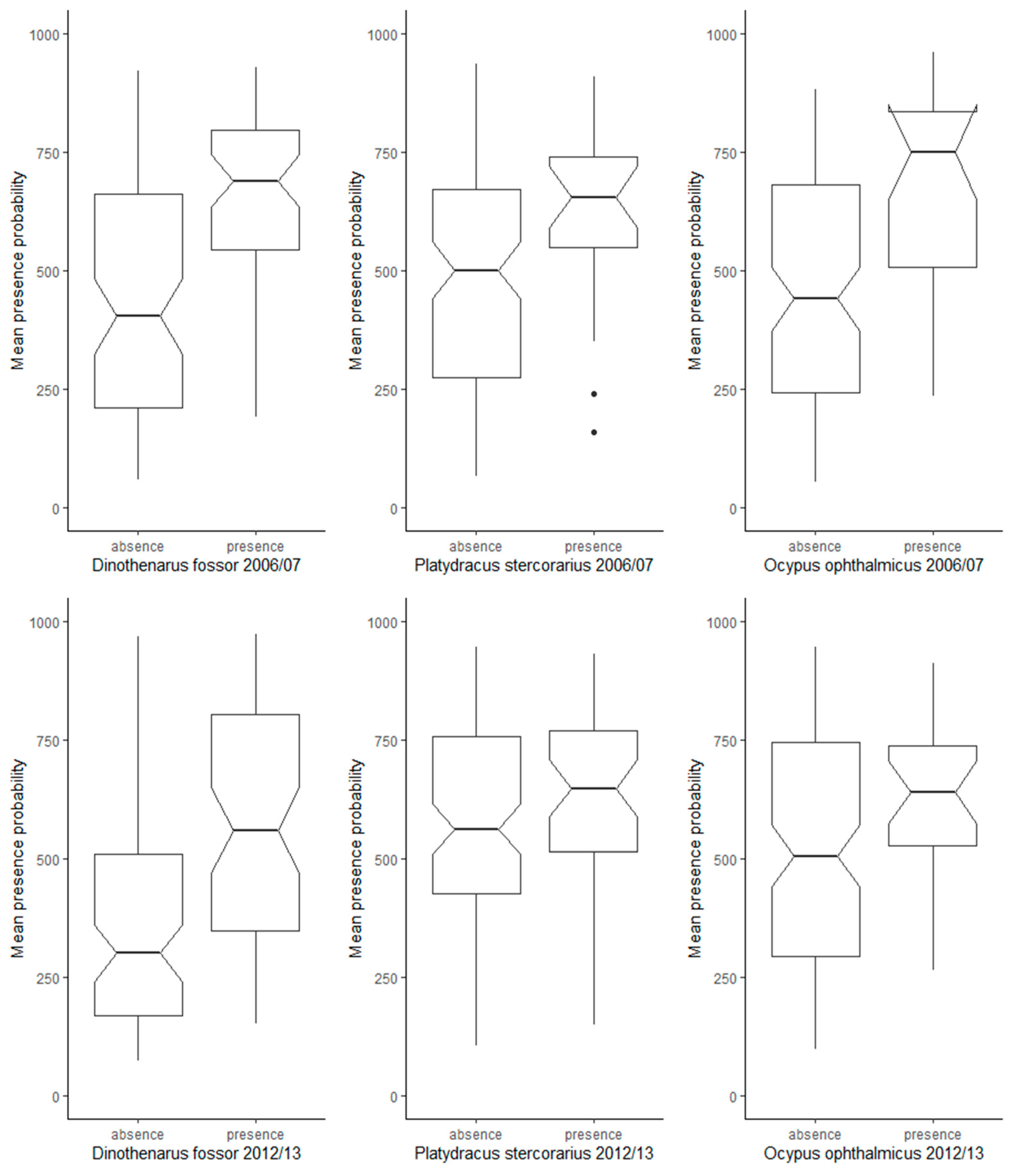
3.2. Effects of Inter-Annual Variability of Species Records on SRS-Based Training Data

The inter-annual variability of the plots in which individuals of the three species were captured (see Section 2.3) together with the inter-annual differences in the SRS data themselves (see Section 2.4) had clear effects on the values and range of the SRS-based model training data (Figure S4). Variability was generally lower for the variables derived from the ASTER GDEM (altitude, eastness, northness, slope, and ruggedness), which were static data for both time periods. On the contrary, the largest differences were found for greenness and wetness, due to variations in ecosystem conditions and seasonal changes as a result of the differences in acquisition dates (the 2006 imagery was acquired 20 days later than the 2013 data). However, variability cannot solely be attributed to differences between the two Landsat data sets. For example, Ocypus ophthalmicus showed considerable variation also for the ASTER GDEM-based variables between 2006–2007 and 2012–2013. Similar differences can be seen for Dinothenarus fossor with respect to eastness. Overall, the subsampling of the full dataset by retaining only one trap per plot did not significantly reduce the variance and range of the environmental variables, apart from few exceptions (Figure S4).

3.3. Variable Importance

Across species, model algorithms, and years, greenness generally had the highest mean variable importance according to correlation analyses between model predictions based on permuted and original datasets, followed by ruggedness (

Table 4. Variable importance according to correlation analyses between model predictions based on permuted and original datasets for all study and model algorithms trained by data collected in 2006–2007 and 2012–2013. Values shown are the mean values across the 50 model repetitions. Cell coloring in dark grey highlights the most important variable and in light grey the second most important one. Abbreviations: GLM, generalized linear model; GAM, generalized additive model; RF, random forest; GBM, generalized boosting model.

	Dinothenarus fossor
Years	2006/2007						2012/2013
Algorithm	GLM	GAM	MAXENT	RF	GBM	Ensemble	GLM	GAM	MAXENT	RF	GBM	Ensemble
Altitude	0.169	0.127	0.175	0.071	0.11	0.117	0.115	0.073	0.105	0.05	0.01	0.048
Northness	0.177	0.182	0.084	0.175	0.002	0.062	0.16	0.234	0.091	0.174	0.022	0.123
Eastness	0.137	0.211	0.02	0.171	0.003	0.079	0.152	0.227	0.035	0.133	0.022	0.11
Slope	0.083	0.05	0.046	0.095	0.001	0.021	0.12	0.053	0.074	0.075	0.022	0.04
Ruggedness	0.122	0.166	0.227	0.179	0.243	0.238	0.138	0.089	0.23	0.182	0.124	0.153
Greenness	0.204	0.182	0.388	0.24	0.642	0.458	0.228	0.237	0.379	0.292	0.792	0.488
Wetness	0.11	0.081	0.06	0.069	0.000	0.024	0.087	0.086	0.085	0.094	0.008	0.038
	Platydracus stercorarius
Years	2006/2007						2012/2013
Algorithm	GLM	GAM	MAXENT	RF	GBM	Ensemble	GLM	GAM	MAXENT	RF	GBM	Ensemble
Altitude	0.107	0.077	0.029	0.063	0.002	0.029	0.136	0.084	0.144	0.076	0.038	0.041
Northness	0.149	0.145	0.087	0.167	0.019	0.083	0.141	0.124	0.063	0.136	0.025	0.07
Eastness	0.133	0.096	0.029	0.155	0.003	0.033	0.149	0.128	0.051	0.139	0.02	0.064
Slope	0.123	0.131	0.005	0.052	0.001	0.019	0.142	0.118	0.156	0.071	0.086	0.076
Ruggedness	0.145	0.165	0.148	0.107	0.174	0.147	0.12	0.152	0.278	0.238	0.299	0.289
Greenness	0.189	0.268	0.516	0.294	0.649	0.532	0.178	0.254	0.227	0.247	0.494	0.403
Wetness	0.152	0.119	0.186	0.162	0.152	0.157	0.134	0.14	0.082	0.092	0.038	0.057
	Ocypus ophthalmicus
Years	2006/2007						2012/2013
Algorithm	GLM	GAM	MAXENT	RF	GBM	Ensemble	GLM	GAM	MAXENT	RF	GBM	Ensemble
Altitude	0.161	0.101	0.074	0.044	0.002	0.052	0.155	0.127	0.222	0.133	0.187	0.096
Northness	0.135	0.194	0.067	0.232	0.054	0.143	0.097	0.238	0.059	0.221	0.108	0.166
Eastness	0.133	0.16	0.043	0.122	0.005	0.076	0.163	0.208	0.025	0.139	0.002	0.081
Slope	0.05	0.076	0.031	0.06	0.057	0.037	0.045	0.054	0.02	0.042	0.027	0.029
Ruggedness	0.208	0.166	0.313	0.266	0.432	0.319	0.199	0.16	0.437	0.225	0.341	0.324
Greenness	0.231	0.2	0.409	0.18	0.425	0.32	0.196	0.144	0.176	0.176	0.313	0.256
Wetness	0.083	0.103	0.063	0.095	0.025	0.053	0.145	0.07	0.062	0.063	0.022	0.048

). This trend was evident also in the ensemble models, for which greenness and ruggedness were always the most important variables, with the only exception being the model built for Platydracus stercorarius in 2006–2007, in which wetness was the second most important variable after greenness. Slope was of only very minor importance in all models. However, slight differences in variable importance between species and years could be detected. For example, topographic variables like ruggedness and northness were more important for Ocypus ophthalmicus than for the other two species, whereas greenness was less important than for Dinothenarus fossor and Platydracus stercorarius. Wetness was found to be an important variable in the ensemble model built for Platydracus stercorarius for the time period 2006–2007, whereas it played only a minor role in all other models. The most consistent pattern across the two time periods considered was found for Dinothenarus fossor, whereas Ocypus ophthalmicus showed the highest variations across model algorithms and between time periods. However, values of importance scores differed, being generally higher for MAXENT and GBM for variables identified as highly important than in the other algorithms. On the other hand, GLMs had the smallest range of variable importance values across variables. The response curves of modelled presence probability relative to each environmental variable showed a strong and positive effect of greenness and a negative effect of ruggedness on species presence for all three species (Figure S5). High wetness values decreased the probability of occurrence of Platydracus stercorarius in the model built for 2006–2007, and a similar but milder effect could be seen for Dinothenarus fossor in 2012–2013. Northness, eastness, and slope had negligible effects on species presence in all six ensemble models. In addition, altitude had weak effects on the SDMs, although some slight differences in altitudinal range between species could be observed in the response curves. Specifically, the models built for Platydracus stercorarius and Ocypus ophthalmicus showed a slight increase of predicted presence probability at higher altitudes (above 2000 m), whereas the trend was reversed in the 2006–2007 Dinothenarus fossor´s model.

3.4. Species Distribution Maps

The area of GPNP for which species distributions could be modelled was larger in 2012–2013 due to a smaller proportion of areas covered by clouds, cloud shadows, and snow in the respective Landsat data set. While the regions predicted as potentially suitable varied to a different extent between the species, valleys generally had higher suitability scores than hillsides or high-altitude plateaus (Figure 3). According to our results, the southern and eastern parts of the study area were generally more suitable compared to the remaining regions. While the six SDMs had high correlation coefficients (Table S1), indicating large similarities in the modelled distributions of the three species, we also observed some differences: Ensemble models built for Ocypus ophthalmicus resulted in a higher predicted occurrence probability in the northeastern part of the study area compared to the other species. The southwestern valleys in the GPNP were also modelled as highly suitable for Ocypus ophthalmicus, whereas their modelled presence probability was intermediate for Platydracus stercorarius and low for Dinothenarus fossor (Figure 3).

Visual comparison of the final SDM maps revealed that modelled distribution patterns across time periods were more similar for Ocypus ophthalmicus than for Dinothenarus fossor and Platydracus stercorarius, which is supported by higher correlation values between the correspondent SDM maps (Table S1). High habitat suitability scores (i.e., above 600) were only obtained for a small proportion of GPNP across all species (below 20% of the study area, Table S2). For Dinothenarus fossor, the area with high suitability scores (>600 to 1000) decreased from 2006–2007 to 2012–2013 (16.4% vs. 8.3%, Table S2). Contrarily, the highly suitable area increased from 8.9% to 16.4% for Platydracus stercorarius and from 11.3% to 19.1% for Ocypus ophthalmicus between the two time periods. Model uncertainty was generally higher in areas with medium to high presence probability and low in areas with lowest predicted suitability (see Figure 3 and Figure S6), showing a similar spatial pattern for the three species. When comparing time periods, overall uncertainty was higher for Dinothenarus fossor and Platydracus stercorarius in the 2012–2013 models, whereas the trend was opposite for Ocypus ophthalmicus.

4. Discussion

The objective of this study was to examine the potential of SRS data to produce species distributions maps of rove beetles with different ecological and functional specialization. A large set of studies predicting species distribution of invertebrates relies on habitat parameters recorded in the field as well as bioclimatic variables [90,91,92]. Others also include SRS-derived information on land use/land cover [93,94,95,96] or variables related to topography (e.g., slope, northness, and eastness, [97]). However, to our knowledge the present study is the first attempt to predict species distribution of beetles in a mountainous region entirely based on SRS data.

4.1. Model Performances to Predict Invertebrate Species Distribution

The presented SDMs can be rated as useful according to Swets [86] and González-Ferreras et al. [88] based on mean AUC and TSS values obtained in the cross-validation step. When comparing different algorithms, regression-based methods (GLM and GAM) had the lowest mean performance, whereas machine-learning methods (RF, GBM, and MAXENT) were found to be the most accurate. GLMs have been widely used in SDM studies [53], but their inability to capture nonlinear responses might be one reason for their poor performance in our study. Otherwise, our results confirmed the robustness and effectiveness of more recently developed machine-learning techniques: Elith et al. [53] showed better performances of GBM and MAXENT compared to GAM and GLM across different species (plants, birds, mammals, and reptiles) and regions; similarly, Marmion et al. [37] and Grenouillet et al. [98] found RF to have the highest accuracy among several tested single algorithm models (among which GLM and GAM) in predicting plant and fish species distributions, respectively. Araújo and New [31] list RF, GBM, and MAXENT as techniques that already incorporate the notion of ensemble forecasting, which could be one of the underlying factors explaining their higher predictive accuracy over regression methods. While the performance of all model algorithms was negatively affected by the small number of presence points used for model fitting, the selection method of pseudo-absences impacted regression and machine-learning techniques differently: Wisz and Guisan [99] and Barbet-Massin et al. [100] showed that a large number (e.g., 10,000) of randomly selected pseudo-absences improved the performance of GLMs and GAMs, hence our spatially stratified selection approach may have influenced the performance of these model types.

Overall, the variability among the five algorithms confirmed the suitability of the chosen ensemble modelling approach, and the evaluation metrics values identified the ensembles as the highest performing models compared to single algorithm models, as also shown by Marmion et al. [37] and Grenouillet et al. [98]. Nonetheless, the comparison of modelled presence probability scores at true absence and presence points revealed that not all ensemble models had high discriminatory power (Figure 2). In particular, the models built for Platydracus stercorarius and Ocypus ophthalmicus in 2012–2013 tended to overestimate distribution ranges, predicting high occurrence probability also at absence locations. This could be due to the small number of presence points available for model training (18 and 12, respectively, Table 1). In fact, models trained using all traps where beetles were captured as presence points (instead of plot-pooled data) had a consistently higher accuracy in discriminating presences from true absence sites. Moreover, distributions of widespread species, such as Platydracus stercorarius, Ocypus ophthalmicus (see description in Section S1), were more difficult to predict compared to those of rare species [50,51]. Nevertheless, the obtained species distribution maps can be considered as quite reliable based on local ecological knowledge, which is becoming increasingly important in ecological modelling in general [101,102]. In particular, the SDMs met our expectations of more similar distribution patterns for Platydracus stercorarius and Dinothenarus fossor, which are both macro-habitat generalists and strongly dependent on vegetated areas, compared to the predicted distribution of Ocypus ophthalmicus, which is less dependent on vegetation (see description in Section S1).

Regarding the spatial resolution of the employed Landsat images and GDEM (30 × 30 m), we assumed adequacy to predict species distribution of invertebrates as other studies employing SRS data were successfully conducted on an even broader spatial scale so far [93,94] (but see Section 4.4). Moreover, despite general recognition of the importance of scale selection in SDMs [103], studies addressing scale directly have found equivocal results: Guisan et al. [104] showed that a 10 times lower resolution of environmental layers used in modelling did not severely affect predictions from SDMs, despite a general decrease in model performance when using explanatory variables at coarser grain size. Nevertheless, as ecological processes are also highly dependent on scale, more research in this direction is needed to better understand the complex relationships between the temporal and spatial variability of species presence records and representation of this variability in SRS data.

4.2. Temporal Variability of Species Presence Records, SRS Data, and Modelled Distribution Ranges

Inter-annual fluctuations in the number of epigeic beetles are a quite common phenomenon found in many works while not completely understood. Indeed, the number of specimens caught by pitfall traps, and consequently the detectability of the species, are linked not only to animal abundance but also to their activity [105,106]. Movement patterns are in turn highly dependent on different factors like temperature and general weather conditions as well as food supply and individual fitness [107]. Furthermore, variations at the micro-habitat scale, including changes in soil moisture, humidity, and in the occurrence of ephemeral resources like prey availability, significantly affect beetles’ abundance, activity, and ultimately detectability [28,108,109]. To reduce yearly variability, we selected species known to be (1) not directly depending on ephemeral resources and (2) nonspecific predators, feeding on various soil arthropods.

The variability of species abundances at trap locations was one reason which led to differences in the values of the SRS-based model predictors at the presence locations between the two time periods (2006–2007 and 2012–2013). The second reason for the observed variations was in the inter-annual differences in environmental conditions, as greenness and wetness were based on different Landsat images for the two time periods. Specifically, the Landsat image was acquired 20 days later in 2006 compared to 2013, explaining the lower values of greenness (Figure S4) associated with differences in vegetation phenology [110]. Such differences in the vegetation-related environmental variables between 2006–2007 and 2012–2013 likely had a comparatively stronger effect on the SDMs built for Dinothenarus fossor and Platydracus stercorarius, for which greenness was highly important. The variation in greenness values could explain the larger differences in predicted species distribution of the two species between time periods when compared to Ocypus ophthalmicus.

In addition, the 2006 Landsat image was also more strongly affected by clouds, shadows, and snow, which further reduced the total area available for modelling in both time periods and limited comparisons about temporal changes in species distributions. The effect of acquisition date of SRS imagery on analyzing species patterns was also shown by other studies [111,112], highlighting the drawbacks of using single SRS imagery representing temporal snapshots and not accounting for intra-annual differences of environmental variables. Analyzing multi-temporal SRS data may be a way to overcome these limitations and has been shown to improve SDMs for marsh bird species [113]. SDMs based on longer composite periods (i.e., multiple years) also showed less deviance from observed species presence/absence field data [114]. While being aware of these problems, the number of suitable SRS imagery was unfortunately restricted in our study and presented SDMs could not be improved in this regard (but see Section 5). Furthermore, radiometric differences between Landsat 5 TM (Thematic Mapper) and Landsat 8 OLI (Operational Land Imager) images may also have caused differences in species predictions [115]. Nevertheless, radiometric differences were overall small in relation to other influencing factors, i.e., phenological differences between the two acquisition dates, and did not affect our overall outcome.

4.3. Importance of SRS Predictors

For all species, SRS-derived greenness was very important. This indicates that vegetated areas are generally preferred by our study species (which is well known at least for Dinothenarus fossor and Platydracus stercorarius, whereas Ocypus ophthalmicus is less dependent on vegetation [47,48,116]). This trend was clearly visible in the variable response curves of all models (Figure S5), in which the modelled probability of species presence increased at higher greenness values. Moreover, ruggedness was identified as the second most important variable in almost all models, negatively affecting the probability of species occurrence. This indicates that penetrability of the terrain determines species distribution: rugged terrain with large variations in elevation, which in turn affect soil thickness and moisture, was less suitable for rove beetles. While known macro- and micro-habitat requirements are rather different (see Box 1 and description in Section S1), the patterns of variable importance and their response curves were fairly similar for the three study species, with greenness and ruggedness being the two most important variables in all ensemble models but one (the 2006–2007 model for Platydracus stercorarius, in which greenness and wetness scored the highest importance values, see Table 4). This indicates that the SRS variables employed in the present study were not entirely capable of depicting the subtle differences in terms of habitat requirements of invertebrate species.

Apart from ruggedness, other topographic-related variables, such as slope, eastness, and northness, had relatively low importance in all models. The effect of wetness in the SDMs is hard to interpret, as it showed contrasting results in the models´ variables response curves. Wetness had a strong negative effect in the 2006–2007 model built for Platydracus stercorarius, but not in 2012–2013. For the other two species, wetness had lower importance scores and a seemingly negative effect on species occurrence, as should be expected in xerophilous species (see Box 1). Altitude, which is typically inversely related to temperature, affected the SDMs very weakly but in different ways for the three species: While we observed negative effects for Dinothenarus fossor (although only for the model referring to 2006–2007), the tendency was opposite for Ocypus ophthalmicus in both time periods, and for Platydracus stercorarius in 2006–2007. These results are in line with our expectations, as the heliophilous species Ocypus ophthalmicus is known to occupy higher altitudes with sunny places above the tree line and to have a broader altitudinal range compared to the other species (see Box 1 and Section S1).

It is difficult to reflect our findings regarding variable importance with respect to other studies, as only very little research has focused on the analysis of spatial patterns of Staphylinidae, either at the community or at the species level. Indeed, the highest number of bibliographic sources is represented by faunistic works, followed by articles considering the role of Staphylinidae as bioindicators, in forest or in agricultural ecosystems [47,48,117,118]. In any case, some general patterns have been found. In particular, it emerged that Staphylinidae are usually more influenced by local factors than landscape-scale features [119]. Community composition and the presence of single species have often been observed as being determined by micro-climate (soil moisture and temperature) and by habitat-related characteristics (vegetation cover and micro-habitat characteristics like decaying material or soil texture) [27,117,120].

4.4. Suggestions for Model Improvement

While the ensemble SDMs outperformed the single algorithm models for all species and years and were thus rated as useful based on the cross-validation results, some suggestions for model improvement can be formulated.

A continuation of the monitoring program in GPNP is recommended (and currently conducted) to assess trends in biodiversity and the impact of environmental changes on species [6,121]. The generation of new species presence and absence information will also improve the performance of SDMs as inter-annual variability in species trapping success can be balanced out. Our decision to train the SDMs on plot-pooled data to avoid issues of pseudo-replication and of spatial correlation reduced our sample size significantly, consequently affecting the discriminatory power of the fitted models. An in-depth analysis of the spectral reflectance characteristics of presence and pseudo-absence data may have further improved model performance as recently shown by Remelgado et al. [122].

The inclusion of additional predictors, such as detailed land cover and grazing intensity maps, could surely improve the models and possibly increase their discernment between the distribution maps of the three species. In our case, these data were unfortunately not available at the right spatial and temporal scale. The availability of environmental variables at finer spatial scale could reduce the problem of spatial autocorrelation between near presence points by enabling the detection of changes in environmental characteristics at a higher resolution, namely within the 50 m of inter-trap distance.

While we here focused on cost-effective explanatory SRS data, recent advances in remote sensing technologies provide the possibility to better account for intra-annual differences in habitat characteristics which likely improve SDMs for our study species in the future. Specifically, Sentinel-1 radar images and Sentinel-2 optical images allow to monitor soil moisture content [123] and vegetation status and composition [124,125] at high spatial resolution and high temporal frequency, respectively. Likewise, high resolution satellite imagery (e.g., PlanetScope) or unmanned aerial vehicles (UAVs) equipped with multi- and hyperspectral sensors as well as laser scanner systems are very promising in this context by providing high resolution data on micro-habitat, vegetation structure, and topography [126,127].

5. Conclusions

The presented findings have important implications for future studies on species distribution modelling. Our results suggest that single time interval studies (as currently often done in SRS-based SDMs) may lead to false assumptions regarding underlying environmental drivers of species distributions. However, a continuation of monitoring is needed to not only track changes in species distribution patterns but also to better account for inter-annual variations due to natural population dynamics and differences in activity patterns. While in the present study, freely available Landsat images were employed, we detected shortages and corresponding implications for species distribution modelling due to the restricted temporal resolution of this data in mountainous regions characterized by high and persistent cloud cover. The limited number of suitable SRS imagery severely restricted our ability to account for intra-annual and inter-annual environmental variability and in turn limited the explanatory power regarding habitat suitability trends over time. However, recent advances in remote sensing technology can solve these problems in future works. Finally, the derived species distribution maps provide valuable information for conservation endeavors in GPNP, e.g., to identify species hot spots and potential connectivity paths inside the protected area. Furthermore, they support environmental change scenarios to identify potential biodiversity losses.

References

1. Körner, C. Why Are There Global Gradients in Species Richness? Mountains Might Hold the Answer Rapoport Effect and Speciation/Extinction Rates. Trends Ecol. Evol. 2000, 15, 513–514. [Google Scholar] [CrossRef]
2. Körner, C.; Paulsen, J.; Spehn, E.M. A Definition of Mountains and Their Bioclimatic Belts for Global Comparisons of Biodiversity Data. Alp. Bot. 2011, 121, 73–78. [Google Scholar] [CrossRef] [Green Version]
3. Díaz, S.; Pascual, U.; Stenseke, M.; Martín-López, B.; Watson, R.T.; Molnár, Z.; Hill, R.; Chan, K.M.A.; Baste, I.A.; Brauman, K.A.; et al. Assessing Nature’s Contributions to People. Science 2018, 359, 270–272. [Google Scholar] [CrossRef] [PubMed] [Green Version]
4. Viviroli, D.; Weingartner, R.; Messerli, B. Assessing the Hydrological Significance of the World’s Mountains. Mt. Res. Dev. 2003, 23, 32–40. [Google Scholar] [CrossRef] [Green Version]
5. Kohler, T.; Wehrli, A.; Jurek, M. Mountains and Climate Change: A Global Concern. Sustainable Mountain Development Series; Centre for Development and Environment (CDE), Swiss Agency for Development and Cooperation (SDC) and Geographica Bernensia: Bern, Switzerland, 2014. [CrossRef]
6. Pocock, M.J.O.; Newson, S.E.; Henderson, I.G.; Peyton, J.; Sutherland, W.J.; Noble, D.G.; Ball, S.G.; Beckmann, B.C.; Biggs, J.; Brereton, T.; et al. Developing and Enhancing Biodiversity Monitoring Programmes: A Collaborative Assessment of Priorities. J. Appl. Ecol. 2015, 52, 686–695. [Google Scholar] [CrossRef] [Green Version]
7. Franklin, J. Mapping Species Distributions: Spatial Inference and Prediction; Cambridge University Press: Cambridge, UK, 2009. [Google Scholar]
8. Sardà-Palomera, F.; Brotons, L.; Villero, D.; Sierdsema, H.; Newson, S.E.; Jiguet, F. Mapping from Heterogeneous Biodiversity Monitoring Data Sources. Biodivers. Conserv. 2012, 21, 2927–2948. [Google Scholar] [CrossRef]
9. Oke, O.A.; Thompson, K.A. Distribution Models for Mountain Plant Species: The Value of Elevation. Ecol. Model. 2015, 301, 72–77. [Google Scholar] [CrossRef]
10. Hijmans, R.J.; Cameron, S.E.; Parra, J.L.; Jones, P.G.; Jarvis, A. Very High Resolution Interpolated Climate Surfaces for Global Land Areas. Int. J. Climatol. 2005, 25, 1965–1978. [Google Scholar] [CrossRef]
11. Luoto, M.; Virkkala, R.; Heikkinen, R.K. The Role of Land Cover in Bioclimatic Models Depends on Spatial Resolution. Glob. Ecol. Biogeogr. 2007, 16, 34–42. [Google Scholar] [CrossRef]
12. Bradley, B.A.; Fleishman, E. Can Remote Sensing of Land Cover Improve Species Distribution Modelling? J. Biogeogr. 2008, 35, 1158–1159. [Google Scholar] [CrossRef]
13. Cord, A.F.; Klein, D.; Mora, F.; Dech, S. Comparing the Suitability of Classified Land Cover Data and Remote Sensing Variables for Modeling Distribution Patterns of Plants. Ecol. Model. 2014, 272, 129–140. [Google Scholar] [CrossRef]
14. Li, X.; Ling, F.; Foody, G.M.; Ge, Y.; Zhang, Y.; Du, Y. Generating a Series of Fine Spatial and Temporal Resolution Land Cover Maps by Fusing Coarse Spatial Resolution Remotely Sensed Images and Fine Spatial Resolution Land Cover Maps. Remote Sens. Environ. 2017, 196, 293–311. [Google Scholar] [CrossRef]
15. He, K.S.; Bradley, B.A.; Cord, A.F.; Rocchini, D.; Tuanmu, M.N.; Schmidtlein, S.; Turner, W.; Wegmann, M.; Pettorelli, N. Will Remote Sensing Shape the next Generation of Species Distribution Models? Remote Sens. Ecol. Conserv. 2015, 1, 4–18. [Google Scholar] [CrossRef] [Green Version]
16. Weiss, D.J.; Walsh, S.J. Remote Sensing of Mountain Environments. Geogr. Compass 2009, 3, 1–21. [Google Scholar] [CrossRef]
17. Liang, L.; Li, X.; Huang, Y.; Qin, Y.; Huang, H. Integrating Remote Sensing, GIS and Dynamic Models for Landscape-Level Simulation of Forest Insect Disturbance. Ecol. Model. 2017, 354, 1–10. [Google Scholar] [CrossRef] [Green Version]
18. Dudov, S.V. Modeling of Species Distribution with the Use of Topography and Remote Sensing Data on the Example of Vascular Plants of the Tukuringra Ridge Low Mountain Belt (Zeya State Nature Reserve, Amur Oblast). Biol. Bull. Rev. 2017, 7, 246–257. [Google Scholar] [CrossRef]
19. Lausch, A.; Bannehr, L.; Beckmann, M.; Boehm, C.; Feilhauer, H.; Hacker, J.M.; Heurich, M.; Jung, A.; Klenke, R.; Neumann, C.; et al. Linking Earth Observation and Taxonomic, Structural and Functional Biodiversity: Local to Ecosystem Perspectives. Ecol. Indic. 2016, 70, 317–339. [Google Scholar] [CrossRef]
20. Turner, W.; Rondinini, C.; Pettorelli, N.; Mora, B.; Leidner, A.K.; Szantoi, Z.; Buchanan, G.; Dech, S.; Dwyer, J.; Herold, M.; et al. Free and Open-Access Satellite Data Are Key to Biodiversity Conservation. Biol. Conserv. 2015, 182, 173–176. [Google Scholar] [CrossRef] [Green Version]
21. Vrieling, A.; Meroni, M.; Darvishzadeh, R.; Skidmore, A.K.; Wang, T.; Zurita-Milla, R.; Oosterbeek, K.; O’Connor, B.; Paganini, M. Vegetation Phenology from Sentinel-2 and Field Cameras for a Dutch Barrier Island. Remote Sens. Environ. 2018, 215, 517–529. [Google Scholar] [CrossRef]
22. Kovacs, E.; Roelfsema, C.; Lyons, M.; Zhao, S.; Phinn, S. Seagrass Habitat Mapping: How Do Landsat 8 OLI, Sentinel-2, ZY-3A, and Worldview-3 Perform? Remote Sens. Lett. 2018, 9, 686–695. [Google Scholar] [CrossRef]
23. Schmidt, J.; Fassnacht, F.E.; Förster, M.; Schmidtlein, S. Synergetic Use of Sentinel-1 and Sentinel-2 for Assessments of Heathland Conservation Status. Remote Sens. Ecol. Conserv. 2018, 4, 225–239. [Google Scholar] [CrossRef] [Green Version]
24. Wulder, M.A.; Masek, J.G.; Cohen, W.B.; Loveland, T.R.; Woodcock, C.E. Opening the Archive: How Free Data Has Enabled the Science and Monitoring Promise of Landsat. Remote Sens. Environ. 2012, 122, 2–10. [Google Scholar] [CrossRef]
25. Wulder, M.A.; Loveland, T.R.; Roy, D.P.; Crawford, C.J.; Masek, J.G.; Woodcock, C.E.; Allen, R.G.; Anderson, M.C.; Belward, A.S.; Cohen, W.B.; et al. Current Status of Landsat Program, Science, and Applications. Remote Sens. Environ. 2019, 225, 127–147. [Google Scholar] [CrossRef]
26. Grimaldi, D.; Engel, M.S. Evolution of the Insect; Cambridge University Press: New York, NY, USA, 2005. [Google Scholar]
27. Bohac, J. Staphylinid Beetles as Bioindicators. Agric. Ecosyst. Environ. 1999, 74, 357–372. [Google Scholar] [CrossRef] [Green Version]
28. Pohl, G.R.; Langor, D.W.; Spence, J.R. Rove Beetles and Ground Beetles (Coleoptera: Staphylinidae, Carabidae) as Indicators of Harvest and Regeneration Practices in Western Canadian Foothills Forests. Biol. Conserv. 2007, 137, 294–307. [Google Scholar] [CrossRef]
29. Assing, V.; Schülke, M. (Eds.) Die Käfer Mitteleuropas, Bd. 4: Staphylinidae (Exklusive Aleocharinae, Pselaphinae Und Scydmaeninae), 2nd ed.; Springer Spektrum: Berlin/Heidelberg, Germany, 2012; ISBN 978-3-8274-1677-3. [Google Scholar]
30. Elith, J.; Leathwick, J.R. Species Distribution Models: Ecological Explanation and Prediction Across Space and Time. Annu. Rev. Ecol. Evol. Syst. 2009, 40, 677–697. [Google Scholar] [CrossRef]
31. Araújo, M.B.; New, M. Ensemble Forecasting of Species Distributions. Trends Ecol. Evol. 2007, 22, 42–47. [Google Scholar] [CrossRef]
32. McCullagh, P.; Nelder, J.A. Generalized Linear Models, 2nd ed.; Monographs on Statistics and Applied Probability; Chapman and Hall/CRC: Boca Raton, FL, USA, 1989; ISBN 9780412317606. [Google Scholar]
33. Hastie, T.; Tibshirani, R. Generalized Additive Models. Stat. Sci. 1986, 249–307. [Google Scholar] [CrossRef]
34. Breiman, L. Random Forests. Mach. Learn. 2001, 45, 5–32. [Google Scholar] [CrossRef] [Green Version]
35. Elith, J.; Leathwick, J.R.; Hastie, T. A Working Guide to Boosted Regression Trees. J. Anim. Ecol. 2008, 77, 802–813. [Google Scholar] [CrossRef]
36. Phillips, S.J.; Dudík, M. Modeling of Species Distributions with Maxent: New Extensions and a Comprehensive Evaluation. Ecography 2008, 31, 161–175. [Google Scholar] [CrossRef]
37. Marmion, M.; Parviainen, M.; Luoto, M.; Heikkinen, R.K.; Thuiller, W. Evaluation of Consensus Methods in Predictive Species Distribution Modelling. Divers. Distrib. 2009, 15, 59–69. [Google Scholar] [CrossRef]
38. Gran Paradiso National Park—Italy. Available online: https://data.lter-europe.net/deims/site/lter_eu_it_109 (accessed on 20 October 2017).
39. Viterbi, R.; Cerrato, C.; Bassano, B.; Bionda, R.; Hardenberg, A.; Provenzale, A.; Bogliani, G. Patterns of Biodiversity in the Northwestern Italian Alps: A Multi-Taxa Approach. Community Ecol. 2013, 14, 18–30. [Google Scholar] [CrossRef]
40. Thomasset, F.; Ottino, M. Parco Nazionale Gran Paradiso. Piano del Parco. Relazione Illustrativa. Available online: http://www.pngp.it/documenti/Piano del parco/PNGP_Relazione.illustrativa.pdf (accessed on 2 March 2018).
41. Cagnacci, F.; Lovari, S.; Meriggi, A. Carrion Dependence and Food Habits of the Red Fox in an Alpine Area. Ital. J. Zool. 2003, 70, 31–38. [Google Scholar] [CrossRef]
42. Poussin, C.; Guigoz, Y.; Palazzi, E.; Terzago, S.; Chatenoux, B.; Giuliani, G. Snow Cover Evolution in the Gran Paradiso National Park, Italian Alps, Using the Earth Observation Data Cube. Data 2019, 4, 138. [Google Scholar] [CrossRef] [Green Version]
43. Marcelino, J.A.P.; Giordano, R.; Borges, P.A.V.; Garcia, P.V.; Soto-Adames, F.N.; Soares, A.O. Distribution and Genetic Variability of Staphylinidae across a Gradient of Anthropogenically Influenced Insular Landscapes. Bull. Insectol. 2016, 69, 117–126. [Google Scholar]
44. Work, T.T.; Klimaszewski, J.; Thiffault, E.; Bourdon, C.; Paré, D.; Bousquet, Y.; Venier, L.; Titus, B. Initial Responses of Rove and Ground Beetles (Coleoptera, Staphylinidae, Carabidae) to Removal of Logging Residues Following Clearcut Harvesting in the Boreal Forest of Quebec, Canada. Zookeys 2013, 258, 31–52. [Google Scholar] [CrossRef] [Green Version]
45. Standen, V. The Adequacy of Collecting Techniques for Estimating Species Richness of Grassland Invertebrates. J. Appl. Ecol. 2000, 37, 884–893. [Google Scholar] [CrossRef] [Green Version]
46. Ribera, I.; Dolédec, S.; Downie, I.S.; Foster, G.N. Effect of Land Disturbance and Stress on Species Traits of Ground Beetle Assemblages. Ecology 2001, 82, 1112–1129. [Google Scholar] [CrossRef]
47. Tagliapietra, A.; Zanetti, A. Staphylinid Beetles in Natura 2000 Sites of Friuli Venezia Giulia. Gortania Botanica Zool. 2012, 33, 97–124. [Google Scholar]
48. Zanetti, A.; Sette, A.; Poggi, R.; Tagliapietra, A. Biodiversity of Staphylinidae (Coleoptera) in the Province of Verona (Veneto, Northern Italy). Mem. Della Soc. Entomol. Ital. 2016, 93, 3–237. [Google Scholar] [CrossRef]
49. Wisz, M.S.; Hijmans, R.J.; Li, J.; Peterson, A.T.; Graham, C.H.; Guisan, A. Effects of Sample Size on the Performance of Species Distribution Models. Divers. Distrib. 2008, 14, 763–773. [Google Scholar] [CrossRef]
50. Van Proosdij, A.S.J.; Sosef, M.S.M.; Wieringa, J.J.; Raes, N. Minimum Required Number of Specimen Records to Develop Accurate Species Distribution Models. Ecography 2016, 39, 542–552. [Google Scholar] [CrossRef]
51. Stockwell, D.R.B.; Peterson, A.T. Effects of Sample Size on Accuracy of Species Distribution Models. Ecol. Model. 2002, 148, 1–13. [Google Scholar] [CrossRef]
52. Hao, T.; Elith, J.; Guillera-Arroita, G.; Lahoz-Monfort, J.J. A Review of Evidence about Use and Performance of Species Distribution Modelling Ensembles like BIOMOD. Divers. Distrib. 2019, 25, 839–852. [Google Scholar] [CrossRef]
53. Elith, J.; Graham, C.H.; Anderson, R.P.; Dudík, M.; Ferrier, S.; Guisan, A.; Hijmans, R.J.; Huettmann, F.; Leathwick, J.R.; Lehmann, A.; et al. Novel Methods Improve Prediction of Species’ Distributions from Occurrence Data. Ecography 2006, 29, 129–151. [Google Scholar] [CrossRef] [Green Version]
54. Fletcher, R.; Fortin, M.J. Spatial Ecology and Conservation Modeling: Applications with R; Springer International Publishing: Cham, Switzerland, 2018. [Google Scholar] [CrossRef]
55. Lobo, J.M.; Jiménez-valverde, A.; Real, R. AUC: A Misleading Measure of the Performance of Predictive Distribution Models. Glob. Ecol. Biogeogr. 2008, 17, 145–151. [Google Scholar] [CrossRef]
56. Earth Resources Observation and Science (EROS) Center Science Processing Architecture (ESPA) on Demand Interface. On Demand Interface. Available online: https://landsat.usgs.gov/sites/default/files/documents/espa_odi_userguide.pdf (accessed on 5 April 2018).
57. Rödder, D.; Nekum, S.; Cord, A.F.; Engler, J.O. Coupling Satellite Data with Species Distribution and Connectivity Models as a Tool for Environmental Management and Planning in Matrix-Sensitive Species. Environ. Manag. 2016, 58, 130–143. [Google Scholar] [CrossRef]
58. Regos, A.; Tapia, L.; Gil-Carrera, A.; Domínguez, J. Monitoring Protected Areas from Space: A Multi-Temporal Assessment Using Raptors as Biodiversity Surrogates. PLoS ONE 2017, 12, e0181769. [Google Scholar] [CrossRef] [Green Version]
59. Crist, E.P.; Cicone, R.C. Application of the Tasseled Cap Concept to Simulated Thematic Mapper Data. Photogramm. Eng. Remote Sens. 1984, 50, 343–352. [Google Scholar]
60. Baig, M.H.A.; Zhang, L.; Shuai, T.; Tong, Q. Derivation of a Tasselled Cap Transformation Based on Landsat 8 At-Satellite Reflectance. Remote Sens. Lett. 2014, 5, 423–431. [Google Scholar] [CrossRef]
61. Myneni, R.B.; Hall, F.G.; Sellers, P.J.; Marshak, A.L. Interpretation of Spectral Vegetation Indexes. IEEE Trans. Geosci. Remote Sens. 1995, 33, 481–486. [Google Scholar] [CrossRef]
62. Parastatidis, D.; Mitraka, Z.; Chrysoulakis, N.; Abrams, M. Online Global Land Surface Temperature Estimation from Landsat. Remote Sens. 2017, 9, 1208. [Google Scholar] [CrossRef] [Green Version]
63. ASTER Global Digital Elevation Map Announcement. Available online: https://asterweb.jpl.nasa.gov/gdem.asp (accessed on 10 May 2018).
64. Hof, A.R.; Jansson, R.; Nilsson, C. The Usefulness of Elevation as a Predictor Variable in Species Distribution Modelling. Ecol. Model. 2012, 246, 86–90. [Google Scholar] [CrossRef]
65. Riley, S.J.; DeGloria, S.D.; Elliot, R. A Terrain Ruggedness Index That Qauntifies Topographic Heterogeneity. Int. J. Sci. 1999, 5, 23–27. [Google Scholar]
66. Dormann, C.F.; Purschke, O.; Márquez, J.R.G.; Lautenbach, S.; Schröder, B. Components of Uncertainty in Species Distribution Analysis: A Case Study of the Great Grey Shrike. Ecology 2008, 89, 3371–3386. [Google Scholar] [CrossRef]
67. Wehn, S.; Johansen, L. The Distribution of the Endemic Plant Primula Scandinavica, at Local and National Scales, in Changing Mountainous Environments. Biodiversity 2015, 16, 278–288. [Google Scholar] [CrossRef] [Green Version]
68. Dirnböck, T.; Dullinger, S.; Grabherr, G. A Regional Impact Assessment of Climate and Land-Use Change on Alpine Vegetation. J. Biogeogr. 2003, 401–417. [Google Scholar] [CrossRef]
69. Pepin, N.; Kidd, D. Spatial Temperature Variation in the Eastern Pyrenees. Weather 2006, 61, 300–310. [Google Scholar] [CrossRef]
70. Kramer-Schadt, S.; Niedballa, J.; Pilgrim, J.D.; Schröder, B.; Lindenborn, J.; Reinfelder, V.; Stillfried, M.; Heckmann, I.; Scharf, A.K.; Augeri, D.M.; et al. The Importance of Correcting for Sampling Bias in MaxEnt Species Distribution Models. Divers. Distrib. 2013, 19, 1366–1379. [Google Scholar] [CrossRef]
71. Cohen, W.B.; Goward, S.N. Landsat’s Role in Ecological Applications of Remote Sensing. Bioscience 2004, 54, 535–545. [Google Scholar] [CrossRef]
72. Carroll, C.; Noss, R.F.; Paquet, P.C. Carnivores as Focal Species for Conservation Planning in the Rocky Mountain Region. Ecol. Appl. 2001, 11, 961–980. [Google Scholar] [CrossRef]
73. Bartel, R.A.; Sexton, J.O. Monitoring Habitat Dynamics for Rare and Endangered Species Using Satellite Images and Niche-Based Models. Ecography 2009, 32, 888–896. [Google Scholar] [CrossRef]
74. Cohen, W.B.; Spies, T.A.; Fiorella, M. Estimating the Age and Structure of Forests in a Multi-Ownership Landscape of Western Oregon, U.S.A. Int. J. Remote Sens. 1995, 16, 721–746. [Google Scholar] [CrossRef]
75. Aguirre-Gutiérrez, J.; Carvalheiro, L.G.; Polce, C.; van Loon, E.E.; Raes, N.; Reemer, M.; Biesmeijer, J.C. Fit-for-Purpose: Species Distribution Model Performance Depends on Evaluation Criteria—Dutch Hoverflies as a Case Study. PLoS ONE 2013, 8, e63708. [Google Scholar] [CrossRef] [Green Version]
76. Thuiller, W.; Georges, D.; Engler, R. Biomod2: Ensemble Platform for Species Distribution Modeling. R Package Version 3.1-48. 2014. Available online: http://cran.r-project.org/package=biomod2 (accessed on 20 May 2019).
77. R Core Team. R: A Language and Environment for Statistical Computing; R Foundation for Statistical Computing: Vienna, Austria, 2014; Available online: http://www.r-project.org/ (accessed on 6 May 2019).
78. Hijmans, R.J. Cross-Validation of Species Distribution Models: Removing Spatial Sorting Bias and Calibration with a Null Model. Ecology 2012, 93, 679–688. [Google Scholar] [CrossRef]
79. Anderson, K.P.; Burnham, D.A. Model Selection and Multi-Model Inference: A Practical Information-Theoretic Approach, 2nd ed.; Springer: Berlin/Heidelberg, Germany, 2002. [Google Scholar] [CrossRef]
80. Wood, S.N. MGCV: Mixed GAM Computation Vehicle with Automatic Smoothness Estimation; R Package Version 1.8. Available online: https://cran.r-project.org/web/packages/mgcv/mgcv.pdf (accessed on 20 October 2019).
81. Merow, C.; Smith, M.J.; Silander, J.A. A Practical Guide to MaxEnt for Modeling Species’ Distributions: What It Does, and Why Inputs and Settings Matter. Ecography 2013, 36, 1058–1069. [Google Scholar] [CrossRef]
82. Phillips, S.J.; Anderson, R.P.; Schapire, R.E. Maximum Entropy Modeling of Species Geographic Distributions. Ecol. Model. 2006, 190, 231–259. [Google Scholar] [CrossRef] [Green Version]
83. Greenwell, B.; Boehmke, B.; Cunningham, J. GBM: Generalized Boosted Regression Models; R Package Version 2.1.5. Available online: https://cran.r-project.org/web/packages/gbm/gbm.pdf (accessed on 20 October 2019).
84. Elith, J.; Ferrier, S.; Huettmann, F.; Leathwick, J. The Evaluation Strip: A New and Robust Method for Plotting Predicted Responses from Species Distribution Models. Ecol. Model. 2005, 186, 280–289. [Google Scholar] [CrossRef]
85. Peterson, A.T.; Papeş, M.; Soberón, J. Rethinking Receiver Operating Characteristic Analysis Applications in Ecological Niche Modeling. Ecol. Model. 2008, 213, 63–72. [Google Scholar] [CrossRef]
86. Swets, J.A. Measuring the Accuracy of Diagnostic Systems. Science 1988, 240, 1285–1293. [Google Scholar] [CrossRef] [Green Version]
87. Allouche, O.; Tsoar, A.; Kadmon, R. Assessing the Accuracy of Species Distribution Models: Prevalence, Kappa and the True Skill Statistic (TSS). J. Appl. Ecol. 2006, 43, 1223–1232. [Google Scholar] [CrossRef]
88. González-Ferreras, A.M.; Barquín, J.; Peñas, F.J. Integration of Habitat Models to Predict Fish Distributions in Several Watersheds of Northern Spain. J. Appl. Ichthyol. 2016, 32, 204–216. [Google Scholar] [CrossRef]
89. Elith, J.; Burgman, M.A.; Regan, H.M. Mapping Epistemic Uncertainties and Vague Concepts in Predictions of Species Distribution. Ecol. Model. 2002, 157, 313–329. [Google Scholar] [CrossRef]
90. Bonn, A.; Schröder, B. Habitat Models and Their Transfer for Single and Multi Species Groups: A Case Study of Carabids in an Alluvial Forest. Ecography 2008, 24, 483–496. [Google Scholar] [CrossRef]
91. De Groot, M.; Rebeušek, F.; Grobelnik, V.; Govedič, M.; Šalamun, A.; Verovnik, R. Distribution Modelling as an Approach to the Conservation of a Threatened Alpine Endemic Butterfly (Lepidoptera: Satyridae). Eur. J. Entomol. 2009, 106, 77–84. [Google Scholar] [CrossRef] [Green Version]
92. Porfirio, L.L.; Harris, R.M.B.; Lefroy, E.C.; Hugh, S.; Gould, S.F.; Lee, G.; Bindoff, N.L.; Mackey, B. Improving the Use of Species Distribution Models in Conservation Planning and Management under Climate Change. PLoS ONE 2014, 9, e113749. [Google Scholar] [CrossRef] [PubMed] [Green Version]
93. Luoto, M.; Kuussaari, M.; Toivonen, T. Modelling Butterfly Distribution Based on Remote Sensing Data. J. Biogeogr. 2002, 29, 1027–1037. [Google Scholar] [CrossRef]
94. Eyre, M.D.; Rushton, S.P.; Luff, M.L.; Telfer, M.G. Predicting the Distributions of Ground Beetle Species (Coleoptera, Carabidae) in Britain Using Land Cover Variables. J. Environ. Manag. 2004, 72, 163–174. [Google Scholar] [CrossRef]
95. Heikkinen, R.K.; Luoto, M.; Kuussaari, M.; Toivonen, T. Modelling the Spatial Distribution of a Threatened Butterfly: Impacts of Scale and Statistical Technique. Landsc. Urban Plan. 2007, 79, 347–357. [Google Scholar] [CrossRef]
96. Widenfalk, L.A.; Ahrné, K.; Berggren, Å. Using Citizen-Reported Data to Predict Distributions of Two Non-Native Insect Species in Sweden. Ecosphere 2014, 5, 1–16. [Google Scholar] [CrossRef] [Green Version]
97. Romo, H.; García-Barros, E.; Márquez, A.L.; Moreno, J.C.; Real, R. Effects of Climate Change on the Distribution of Ecologically Interacting Species: Butterflies and Their Main Food Plants in Spain. Ecography 2014, 37, 1063–1072. [Google Scholar] [CrossRef]
98. Grenouillet, G.; Buisson, L.; Casajus, N.; Lek, S. Ensemble Modelling of Species Distribution: The Effects of Geographical and Environmental Ranges. Ecography 2011, 34, 9–17. [Google Scholar] [CrossRef]
99. Wisz, M.S.; Guisan, A. Do Pseudo-Absence Selection Strategies Influence Species Distribution Models and Their Predictions? An Information-Theoretic Approach Based on Simulated Data. BMC Ecol. 2009, 9, 8. [Google Scholar] [CrossRef] [PubMed] [Green Version]
100. Barbet-Massin, M.; Jiguet, F.; Albert, C.H.; Thuiller, W. Selecting Pseudo-Absences for Species Distribution Models: How, Where and How Many? Methods Ecol. Evol. 2012, 3, 327–338. [Google Scholar] [CrossRef]
101. Krueger, T.; Page, T.; Hubacek, K.; Smith, L.; Hiscock, K. The Role of Expert Opinion in Environmental Modelling. Environ. Model. Softw. 2012, 36, 4–18. [Google Scholar] [CrossRef]
102. Bélisle, A.C.; Asselin, H.; Leblanc, P.; Gauthier, S. Local Knowledge in Ecological Modeling. Ecol. Soc. 2018, 23, 14. [Google Scholar] [CrossRef]
103. Anderson, C.B. Biodiversity Monitoring, Earth Observations and the Ecology of Scale. Ecol. Lett. 2018, 21, 1572–1585. [Google Scholar] [CrossRef]
104. Guisan, A.; Graham, C.H.; Elith, J.; Huettmann, F.; Dudik, M.; Ferrier, S.; Hijmans, R.; Lehmann, A.; Li, J.; Lohmann, L.G.; et al. Sensitivity of Predictive Species Distribution Models to Change in Grain Size. Divers. Distrib. 2007, 13, 332–340. [Google Scholar] [CrossRef]
105. Thiele, H.-U. Carabid Beetles in Their Environments; Springer: Berlin/Heidelberg, Germany, 1977; ISBN 978-3-642-81156-2. [Google Scholar]
106. Saska, P.; van der Werf, W.; Hemerik, L.; Luff, M.L.; Hatten, T.D.; Honek, A. Temperature Effects on Pitfall Catches of Epigeal Arthropods: A Model and Method for Bias Correction. J. Appl. Ecol. 2013, 50, 181–189. [Google Scholar] [CrossRef] [Green Version]
107. Southwood, T.R.E.; Henderson, P.A. Ecological Methods, 3rd ed.; Blackwell Science: Hoboken, NJ, USA, 2000; ISBN 978-0-632-05477-0. [Google Scholar]
108. Buse, A.; Good, J.E.G. The Effects of Conifer Forest Design and Management on Abundance and Diversity of Rove Beetles (Coleoptera: Staphylinidae): Implications for Conservation. Biol. Conserv. 1993, 64, 67–76. [Google Scholar] [CrossRef]
109. Hoffmann, H.; Michalik, P.; Görn, S.; Fischer, K. Effects of Fen Management and Habitat Parameters on Staphylinid Beetle (Coleoptera: Staphylinidae) Assemblages in North-Eastern Germany. Insect Conserv. 2016, 20, 129–139. [Google Scholar] [CrossRef]
110. Fontana, F.; Rixen, C.; Jonas, T.; Aberegg, G.; Wunderle, S. Alpine Grassland Phenology as Seen in AVHRR, VEGETATION, and MODIS NDVI Time Series—A Comparison with in Situ Measurements. Sensors 2008, 8, 2833–2853. [Google Scholar] [CrossRef] [PubMed] [Green Version]
111. Bino, G.; Levin, N.; Darawshi, S.; Van Der Hal, N.; Reich-Solomon, A.; Kark, S. Accurate Prediction of Bird Species Richness Patterns in an Urban Environment Using Landsat-Derived NDVI and Spectral Unmixing. Int. J. Remote Sens. 2008, 29, 3675–3700. [Google Scholar] [CrossRef]
112. Sheeren, D.; Bonthoux, S.; Balent, G. Modeling Bird Communities Using Unclassified Remote Sensing Imagery: Effects of the Spatial Resolution and Data Period. Ecol. Indic. 2014, 43, 69–82. [Google Scholar] [CrossRef]
113. Pickens, B.A.; King, S.L. Linking Multi-Temporal Satellite Imagery to Coastal Wetland Dynamics and Bird Distribution. Ecol. Model. 2014, 285, 1–12. [Google Scholar] [CrossRef]
114. Cord, A.; Klein, D.; Dech, S. The Impact of Inter-Annual Variability in Remote Sensing Time Series on Modelling Tree Species Distributions. In Proceedings of the 6th International Workshop on the Analysis of Multi-Temporal Remote Sensing Images (Multi-Temp), Trento, Italy, 12–14 July 2011. [Google Scholar] [CrossRef]
115. Young, N.E.; Anderson, R.S.; Chignell, S.M.; Vorster, A.G.; Lawrence, R.; Evangelista, P.H. A Survival Guide to Landsat Preprocessing. Ecology 2017, 98, 920–932. [Google Scholar] [CrossRef] [Green Version]
116. Zanetti, A.; Tagliapietra, A. Studi Sulle Taxocenosi Di Staphylinidae in Boschi Di Latifoglie Italiani (Coleoptera, Staphylinidae). Stud. Trentini Sci. Nat. Acta Biol. 2004, 81, 207–231. [Google Scholar]
117. Balog, A.; Markó, V.; Imre, A. Farming System and Habitat Structure Effects on Rove Beetles (Coleoptera: Staphylinidae) Assembly in Central European Apple and Pear Orchards. Biologia 2009, 64, 343–349. [Google Scholar] [CrossRef]
118. Lupi, D.; Colombo, M.; Facchini, S. The Ground Beetles (Coleoptera: Carabidae) of Three Horticultural Farms in Lombardy, Northern Italy. Boll. Zool. Agr. Bachic. 2006, 39, 193–209. [Google Scholar]
119. Dauber, J.; Purtauf, T.; Allspach, A.; Frisch, J.; Voigtländer, K.; Wolters, V. Local vs. Landscape Controls on Diversity: A Test Using Surface-Dwelling Soil Macroinvertebrates of Differing Mobility. Glob. Ecol. Biogeogr. 2005, 14, 213–221. [Google Scholar] [CrossRef]
120. Magura, T.; Nagy, D.; Tóthmérész, B. Rove Beetles Respond Heterogeneously to Urbanization. J. Insect Conserv. 2013, 17, 715–724. [Google Scholar] [CrossRef] [Green Version]
121. Raxworthy, C.J.; Martinez-Meyer, E.; Horning, N.; Nussbaum, R.A.; Schneider, G.E.; Ortega-Huerta, M.A.; Peterson, A.T. Predicting Distributions of Known and Unknown Reptile Species in Madagascar. Nature 2003, 426, 837–841. [Google Scholar] [CrossRef] [PubMed] [Green Version]
122. Remelgado, R.; Leutner, B.; Safi, K.; Sonnenschein, R.; Kuebert, C.; Wegmann, M. Linking animal movement and remote sensing—Mapping resource suitability from a remote sensing perspective. Remote Sens. Ecol. Conserv. 2017, 4, 211–224. [Google Scholar] [CrossRef] [Green Version]
123. Alexakis, D.D.; Mexis, F.D.K.; Vozinaki, A.E.K.; Daliakopoulos, I.N.; Tsanis, I.K. Soil Moisture Content Estimation Based on Sentinel-1 and Auxiliary Earth Observation Products. A Hydrological Approach. Sensors 2017, 17, 1455. [Google Scholar] [CrossRef] [Green Version]
124. Frampton, W.J.; Dash, J.; Watmough, G.; Milton, E.J. Evaluating the Capabilities of Sentinel-2 for Quantitative Estimation of Biophysical Variables in Vegetation. ISPRS J. Photogramm. Remote Sens. 2013, 82, 83–92. [Google Scholar] [CrossRef] [Green Version]
125. Belgiu, M.; Csillik, O. Sentinel-2 Cropland Mapping Using Pixel-Based and Object-Based Time-Weighted Dynamic Time Warping Analysis. Remote Sens. Environ. 2018, 204, 509–523. [Google Scholar] [CrossRef]
126. Manfreda, S.; McCabe, M.F.; Miller, P.E.; Lucas, R.; Madrigal, V.P.; Mallinis, G.; Dor, E.B.; Helman, D.; Estes, L.; Ciraolo, G.; et al. On the Use of Unmanned Aerial Systems for Environmental Monitoring. Remote Sens. 2018, 10, 641. [Google Scholar] [CrossRef] [Green Version]
127. Cruzan, M.B.; Weinstein, B.G.; Grasty, M.R.; Kohrn, B.F.; Hendrickson, E.C.; Arredondo, T.M.; Thompson, P.G. Small Unmanned Aerial Vehicles (Micro-Uavs, Drones) in Plant Ecology. Appl. Plant Sci. 2016, 4, 160041. [Google Scholar] [CrossRef]
Figure 1. Study area and sampling design for long-term biodiversity monitoring efforts. (a) Location of Gran Paradiso National Park. A buffer of 1 km was added to the official boundaries of the park to avoid edge effects when modelling species distributions. (b) Locations of transects within the park boundaries. (c) Schematic representation of the distribution of plots along a transect (following contour lines). (d) Locations of pitfall traps within each plot.
Remotesensing 12 00080 g001
Figure 2. Comparison of modelled presence probabilities (ensemble models) at presence (traps in which individuals of each target species were captured) and absence locations (traps without captured individuals, not used for model training) for the time periods 2006–2007 and 2012–2013.
Remotesensing 12 00080 g002
Figure 3. Species distribution likelihood for each species in 2006–2007 and 2012–2013 based on the ensemble models. Locations of the plots used as presence points for model training are shown to emphasize the variability of input data. Coordinates shown are based ETRS (European Terrestrial Reference System) 1989 LAEA (Lambert Azimuthal Equal-Area) projection.
Remotesensing 12 00080 g003