Mapping the Seabed and Shallow Subsurface with Multi-Frequency Multibeam Echosounders


1
Acoustics Group, Faculty of Aerospace Engineering, Delft University of Technology, 2629 HS Delft, The Netherlands
2
Department of Applied Geology and Geophysics, Deltares, 3508 AL Utrecht, The Netherlands
*
Author to whom correspondence should be addressed.
Remote Sens. 2020, 12(1), 52; https://doi.org/10.3390/rs12010052
Submission received: 21 October 2019
/
Revised: 18 November 2019
/
Accepted: 15 December 2019
/
Published: 21 December 2019
(This article belongs to the Section Ocean Remote Sensing)
Abstract
:Multi-frequency multibeam backscatter (BS) has indicated, in particular for fine sediments, the potential for increasing the discrimination between different seabed environments. Fine sediments are expected to have a varying signal penetration within the frequency range of modern multibeam echosounders (MBESs). Therefore, it is unknown to what extent the multispectral MBES data represent the surface of the seabed or different parts of the subsurface. Here, the effect of signal penetration on the measured multi-frequency BS and bathymetry is investigated. To this end, two multi-frequency datasets (90 to 450 kHz) were acquired with an R2Sonic 2026 MBES, supported by ground-truthing, in the Vlietland Lake and Port of Rotterdam (The Netherlands). In addition, a model to simulate the MBES bathymetric measurements in a layered medium is developed. The measured bathymetry difference between the lowest (90 kHz) and highest frequency (450 kHz) in areas with muddy sediments reaches values up to 60 cm dependent on the location and incident angle. In spatial correspondence with the variation in the depth difference, the BS level at the lowest frequency varies by up to 15 dB for the muddy sediments while the BS at the highest frequency shows only small variations. A comparison of the acoustic results with the ground-truthing, geological setting and model indicates that the measured bathymetry and BS at the different frequencies correspond to different parts of the seabed. However, the low-frequency BS cannot be directly related to a subsurface layer because of a significant sound attenuation in the upper layer. The simulation of the MBES bottom detection indicates that the bathymetry measured at the highest and lowest frequency can be used to determine the thickness of thin layers (∼20 cm). However, with an increasing layer thickness, the bottom detection becomes more sensitive to the incident angle and small variations in the sediment properties. Consequently, an accurate determination of the layer thickness is hampered. Based on this study, it is highly recommended to analyze multi-frequency BS in combination with the inter-frequency bathymetry difference to ensure a correct interpretation and classification of multi-frequency BS data.

1. Introduction
Multibeam echosounders (MBESs) are the most efficient and widely used sonar technology for seabed mapping. Beamforming in the across-track direction enables measurements of the signal travel time to the seabed for a large number of beam angles. As such, it provides detailed and extensive information about the seabed bathymetry. The MBES also co-registers the intensity of the returning signal for each beam. Applying geometric and radiometric corrections to the received signal, a measure of the acoustic backscatter (BS) strength can be retrieved [1]. This is a measure of the sound that is scattered or reflected from the water-sediment interface (interface scattering) and from the sediment volume (volume scattering) back towards the transmitter [2,3]. Both mechanisms are controlled by the difference in density and sound velocity between the water and the sediment. In addition, interface scattering is mainly caused by the roughness of the seabed and volume scattering depends on the heterogeneity of the shallow subsurface [4]. The BS strength also varies with the incident angle, known as the angular response [5]. Furthermore, the relation between the acoustic frequency and roughness wavelength affects the interaction of the sound with seabed [3]. While higher frequencies are more sensitive to the seabed roughness, lower frequency signals are more affected by volume heterogeneities due to lower sound attenuation, resulting in an increased signal penetration, in the sediment.
Generally, the MBES operates in a narrow band around the central frequency and therefore the BS data are collected at a single frequency (i.e., monochromatic). Monochromatic BS data collected with a MBES have been used for two decades to remotely characterize or classify seabed sediments or habitats via sophisticated classification algorithms [6,7,8,9]. However, previous studies have shown that monochromatic BS can lead to ambiguous results when classifying different seabed environments [10,11,12]. That means different sediment compositions or mixtures have similar acoustic properties at the same frequency. According to theoretical [4,13] and experimental [14] research of acoustic BS and considering the analogy to satellite remote imaging, where backscattered light is collected over a wide frequency spectrum of electromagnetic waves, the use of BS data at different frequencies (i.e., multispectral) is promising to further reduce ambiguous sediment classification results.
Recent research studies employing multispectral BS data have shown improvements in sediment and habitat mapping. The acquisition of multispectral BS data has been achieved by using either different acoustic sensors (i.e., MBES and Side-scan sonar) [15], various MBESs [16], or a single broadband MBES running multiple track lines [17]. New developments in marine sonar technology allow the MBES to collect spatially and temporally co-located BS data at multiple frequencies (i.e., 90 to 450 kHz) using a single system. The first research studies, employing such a MBES, have also indicated a potential to increase the discrimination between different seabed environments using multi-frequency BS data [18,19,20,21]. In these studies different BS patterns at various frequencies (100, 200, and 400 kHz), indicating the benefits of multiple frequencies, were mainly observed for areas consisting of fine sediments (mud). The different BS patterns were potentially caused by coarse, dredge spoil material below a mud layer, and sensed due to an increased signal penetration of the lower frequencies. With respect to the typical frequency range of modern MBESs (12 to 700 kHz), different signal penetrations, in particular for fine sediments, are expected [22]. Deimling et al. [23] measured a signal penetration of up to 12 m in muddy deposits with a 12 kHz MBES. For frequencies around 100 kHz a penetration between 0.1 m to 1 m in fine sediments is expected [24]. Simulations based on the empirical equations of Hamilton [22] showed that, in particular, between fine sediments ranging from gravelly mud (4) to clay (9) the signal penetration of a100 kHz signal due to attenuation differs enormously (∼1 m) [18]. This indicates the high sensitivity of the acoustic penetration to small changes in sediment properties. In another study by Fonseca [24], high BS levels in muddy sediments were measured, which is counter-intuitive to the general knowledge of muddy sediments corresponding to a low BS level [13]. They explained this observation, among others, with an increased penetration of the 95 kHz signal and the contribution of subsurface layering to the measured BS level.
These findings demonstrate that not only changes in the surficial sediment, to which one frequency is more sensitive than another, result in different BS patterns between the frequencies. But they also seem to indicate that when shallow sediment layering below fine sediments exists, the observed frequency dependency of BS may result from the ensonification of different sediments at different depths due to varying signal penetration at the transmitted frequencies. With the increasing use of multi-frequency BS data for sediment and habitat mapping, it is necessary to investigate what part of the seabed or subsurface is represented by the measured BS data to avoid ambiguous classification results. In particular, for fine sediments, the multi-frequency BS data and consequently the acoustic classification map might represent a 3D image of the surficial seabed and the shallow subsurface as argued by Gaida et al. [18].
This study seeks to extend the knowledge about multispectral MBES data by investigating the effect of frequency-dependent signal penetration on multi-frequency BS and bathymetry data. In particular, the effect of sediment layering on the BS data is examined. To this end, we acquired two multi-frequency BS dataset (90 to 450 kHz) with an R2Sonic 2026 MBES in a freshwater lake and in the Port of Rotterdam in the Netherlands. Both study areas consist, to a large extent, of surficial fine (muddy) sediments. In addition, we collected ground truth information via Van Veen sampling and video footage in the Vlietland Lake and rheometric profiling (i.e., subsurface density) in the Port of Rotterdam to support the acoustic results. To gain an improved understanding and interpretation of multispectral MBES data, a layered BS model, based on [25], is used and an algorithm to model the MBES bathymetric measurements in a layered medium is developed.
2. Study Area and Data
2.1. Regional Setting
2.1.1. Vlietland Lake
The Vlietland Lake is a man-made freshwater lake in the western part of the Netherlands (Figure 1c). The lake is a former sandpit used for the extraction of sand since 1970 and has recently become a recreation area and nature reserve. The lake was dredged through several geological layers ranging from peaty to gravelly sand layers. The current water depth ranges from 4 to 32 m below Normal Amsterdam Peil (NAP). The majority of the lakebed is located in the Kreftenheye formation consisting of fluvial coarse sand (0.2 to 2 mm) and gravel (5.6 to 63 mm) [26]. Around the lake, the Kreftenheye formation is located between approximately 17 to 36 m below NAP. The surficial sediments of the lake towards the shoreline consist of fine to medium sand with a varying percentage of shells, coarse sand, and mud ( = 70 to 310 m). The surficial sediments away from the shoreline consist of mud with a small percentage of fine sand ( = 18 to 26 m and defined as sandy mud after Folk [27]). With the finalization of the sand extraction activities, the muddy sediments were deposited on the sand and gravel sediments of the Kreftenheye formation probably due to aeolian sediment transport and sedimentation of organic matter.
2.1.2. Port of Rotterdam
The Port of Rotterdam is located in the Rhine-Meuse Estuary, which is defined as a transition zone between a river and marine environment (Figure 1d). Therefore, the Port of Rotterdam has a deposition of fluvial and marine sediments. It requires intensive maintenance dredging to ensure port accessibility for the vessels with the highest draft which results in 12 to 15 million m3 of dredged sediment per year [28]. The material to be dredged consists of alluvial sediments (mainly silt) from the Rhine and Meuse as well as sand and marine silts originating from the southern part of the North Sea. The survey area covers a man-made pit used as a sediment trap for water injection dredging (WID). The last WID was conducted in October 2018 and the comparison with previous bathymetry measurements combined with the analysis of the bed samples indicated that the sediment trap is refilled with muddy sediments ( = 15 m and defined as sandy mud after Folk [27]). The current water depth of the study area ranges from 19 to 26 m below NAP.
2.2. Multibeam Data Acquisition
Two multi-frequency MBES datasets were acquired with an R2Sonic 2026 in the Vlietland Lake and Port of Rotterdam in September 2018 and January 2019, respectively (The Netherlands). The data were collected at five different frequencies between 90 and 450 kHz on a ping-by-ping basis. Further crucial survey parameters are listed in Table 1. The MBES was pole mounted and operated with the R2Sonic controller and the acquisition software Qinsy. An iXblue Octans 3000 motion sensor and iXblue Phins provided real-time heading, roll, pitch, and heave for the Port of Rotterdam and Vlietland Lake, respectively. For both study areas, a Trimble SPS855 GNSS receiver provided real-time kinematic positioning with a horizontal and vertical accuracy of 1 and 2 cm, respectively. Regularly performed CTD (Conductivity, Temperature, and Depth) measurements gave temporal and spatial measurements of the water column for ray-tracing and sound absorption. The absorption depth profile was calculated using the equation from Francois and Garrison [29]. The Port of Rotterdam and Vlietland Lake datasets consist of 5 and 15 track lines resulting in an area of km × km and km × km, respectively (Figure 1c,d). To guarantee sufficient data coverage at each frequency, an overlap of about 120% of adjacent lines was ensured and the vessel speed was kept between 2 and 3 knots.
2.3. Ground Truth Data
In the Vlietland Lake, 12 grab samples were taken with a small Van Veen sampler. This device has a grasping area of maximum 250 cm2 and is expected to reach a penetration depth between 10 to 20 cm in muddy sediments. The sample locations were selected based on the observed MBES BS patterns. The samples were photographed and subsampled for a grain size analysis. The grains smaller than 1 mm were analyzed by laser diffraction and the grains larger than 1 mm were analyzed by sieving. The median grain size () was calculated for the entire grain size spectrum. We classified the samples according to Folk [27], as sandy mud (sM), sandy mud with shells (sM SH), muddy sand with shells (mS SH), and sand with shells (S SH). In addition, video transects were carried out to obtain a visual overview of the seabed in the Vlietland Lake.
In the Port of Rotterdam, depth profiles of in situ sediment properties, i.e., density and yield stress, were measured with a pre-calibrated rheometric profiler before the MBES acquisition. In the same area, Van Veen samples were acquired in previous measurement campaigns. It was seen that sediment grain size distribution do not to vary significantly in time and, therefore, we consider the measurements as representative.
3. Method
Section 3.1 outlines the processing of the measured multibeam data and explains the generation of the corresponding maps and figures. Section 3.2 briefly describes the layered BS model developed by Guillon and Lurton [25]. This model is an extension of the APL-model [30] and used to model the BS strength of a layered medium. The layered BS model is employed to support the interpretation of the measured BS data. Section 3.4 gives a detailed description of the bottom detection model developed in this study. This model simulates the sound transmission and reception at the MBES as well as the sound propagation and scattering in the media. Within the bottom detection model, the APL-model and its extension provide the BS strength for the surficial and buried sediment. The model is used to simulate the bathymetric measurements of a MBES in a layered medium in order to support the interpretation of the measured bathymetry.
3.1. Multibeam Data Processing
Bathymetric data processing is carried out with the software Qimera, applying manual and spline filtering to remove sounding artifacts. The bathymetry data is then separated per frequency and gridded into a m and m grid using the GIS software packages ARCmap 10.5 for the Vlietland Lake and Port of Rotterdam, respectively. Following this, the bathymetry grids obtained for the different frequencies are subtracted from each other to calculate the difference in the measured bathymetry between the frequencies.
The multi-frequency BS data are processed with an in-house developed processing algorithm written in Matlab. In this study, the so-called "BS intensity per beam value" representing the return level at the bottom detection point [31] and the entire time series signal are used. To retrieve a physical reasonable BS level from the measured data, the processing chain introduced by Gaida et al. [18] is applied. The measured data is corrected for the receiving gain, actual source level, transducer sensitivity per frequency (frequency response) and transmission loss including geometrical spreading and sound absorption. The BS level at the bottom detection is additionally corrected for the ensonified footprint and the seabed morphology. The frequency response correction term, which is used to compensate for the transducer sensitivity per frequency, is based on a theoretical calculation and the level of uncertainty is unknown. Therefore, a precise comparison of the decibel values between the frequencies is hampered. In addition, no absolute or relative calibration is applied to the MBES and the data has thus to be considered as a relative measure of the BS strength. Once the BS processing is completed, the BS mosaics are generated by calculating an averaged angular response curve (ARC) over a sliding window of 100 pings, subtracting the averaged ARC from the data and then normalizing the BS level with the averaged BS level between 30 and 60 for starboard and port side separately.
The calculation of the measured bathymetric uncertainties is carried out by dividing the survey area into surface patches each consisting of a few consecutive pings (i.e., 7 pings) in the along-track direction and a few beams around the central beam angle in the across-track direction (i.e., interval of 1). To eliminate the contribution of the morphology, a bi-quadratic or linear function is fitted to the measurements within each surface patch [32]. The unknown parameters (i.e., coefficients of the function) are derived in a least-square sense. Here, the bathymetric uncertainty is the standard deviation (68% confidence interval) obtained from the square root of the least-squares estimate of the variance component [33] and accounted for the potential presence of slopes. The degree of the fit function (bi-quadratic or linear) is based upon the curvature C, which is a measure for the surface patch deviation from a flat plane. For the data acquired, it is seen that corresponds to steep slopes. Therefore, for a surface patch with a linear function is used for the fit, otherwise a bi-quadratic fit is employed.
3.2. Layered Backscatter Model
The layered BS model developed by Guillon and Lurton [25] is based on the combination of a classical scattering model (called Jackson model [13] or APL-model [30]) and sound propagation inside a fluid layered media. In the APL-model, the BS strength , received from the backscattering cross-section via , is modeled as a contribution of the rough seabed (roughness scattering ) and the semi-infinite volume heterogeneity (volume scattering ) [13]
with and . This means that the model requires eight input parameters: incident angle , frequency f, density , sound velocity c, attenuation coefficient , spectral exponent , spectral strength , and volume scattering parameter . The density , the sound velocity c, and the attenuation coefficient need to be known for both the water and sediment.
The APL-model is considered valid for frequencies between 10 and 100 kHz. The limitation is mainly caused by the roughness scattering model. The focus in this study is mostly on fine sediments where volume scattering dominates over interface scattering and, therefore, we consider the model to be applicable also for higher frequencies.
To model the BS of a layered medium, Guillon and Lurton [25] modified the APL-model to account for the layering effect on sound reflection and scattering. The of the surficial and the buried layer is modeled individually using the APL-model and accounting for the layering effect. The individual contributions of both layers are summed coherently. A buried sediment layer affects and at both the water-sediment and the buried interface. The calculation of corresponding to the upper layer is modified to account for the finite thickness. An impedance adaption and angular refraction correction is implemented for both scattering mechanisms when calculating the scattering of the second layer. Furthermore, the BS is transferred from the buried interface to the sediment-water interface by accounting for the sound propagation in the layered medium. Therefore, a transfer-coefficient is calculated which is based on the transmission coefficient and the sound absorption within the layered medium. For further theoretical details and corresponding equations, we refer to [25,30].
3.3. Model Parameter Selection
For this study a two-layered geophysical model consisting of the water column and two sediment layers is considered. The values for the input-variables are displayed in Table 2. The parameters , c, and for the water column are based on the CTD-measurements taken in the Vlietland Lake. For the sediment, the empirical equations established by Hamilton [22] are used to estimate , c and from the median grain size. In agreement with recommendations by the APL-model [30], we relate , and to the median grain size.
We model two scenarios with a median grain size of 6 (16 m) and 9 (2 m) for the surficial sediment while the buried sediment has a median grain size of −1 (2 mm) for both scenarios. The median grain size of 6 represents the surficial sandy mud at both sites and the median grain size of −1, associated to sandy gravel [30], is assumed to represent the buried sediment layer in the Vlietland Lake (Section 2.1). A median grain size of 9, associated with clay [34], represents a second scenario to investigate the effect of even finer sediments on the BS strength and bottom detection.
3.4. Bottom Detection Model
In the bottom detection model the different layers are modeled by a large set of discrete scatterers each of them scattering the transmitted sound pulse to generate the received pressure signal. Following the approach of the APL-model, roughness and volume scattering are associated with the location of the interface scatterer although volume scattering is originated from the underlying volume. The backscattered signal is derived by a coherent summation of the received signal from the scatterers falling within the instantaneously ensonified area [35]. The sound pressure of the received MBES signal at a given time instant t and steering angle is given as
where is the transmitted sound pressure signal, is the beam pattern and J is the number of scatterers j falling in the instantaneously ensonified area at time t. is the target’s backscattering cross section of scatterer j at incident angle . The term accounts for the two-way geometrical spreading (denominator) and attenuation of the signal within a dissipative propagation medium (nominator). The transmitted sound pressure signal by the MBES can be expressed as a sinusodial pressure wave [36]
where is the pulse length, is the root mean square pressure (rms) of the transmitted pulse and is a Hanning tapering function to reflect a smooth signal. The arrival time of each scatterer is , where h is the water depth below the MBES, is the sound speed in water and is the incident angle. Assuming a homogeneous water column, the calculation of does not require consideration of the sound refraction. The receiving beam pattern is expressed as [36]
where M is the number of receiving element m, k is the wave number of the transmitted signal and is the receiver array length (Table 3).
The following explains how to relate the term in Equation (2) to the backscattering cross-section . First of all, the square root relates intensity to pressure values for the target’s backscattering cross-section via
where , , , and denote the intensities and rms pressures of the backscattered and the incident wave. The target’s backscattering cross-section is related to the backscattering cross-section via the instantaneously ensonified area as follows:
where is obtained from the APL-model (Equation (1), Section 3.2). In order to account for the statistical fluctuation inherent to the scattering process, is modeled as a Rayleigh distributed variable [37]. Here, (with in degree) represents the sector of a circle with a radius x (i.e., distance in across-track direction) and an opening angle (i.e., represents the beam opening angle at transmission, with the transmitter array length). By substituting (with in radians) into Equation (6), it follows
which becomes for the discrete scatterer case
The target’s backscattering cross-section at each scatterer j can thus be expressed as
where the incident angle of each scatterer is connected to the slant range or the water depth h via the horizontal distance of each scatterer toward the receiver: = or = .
Here, as seen from the relation established between Equations (6)–(8), the instantaneously ensonified area, containing J scatterers, is bounded in the horizontal direction (across-track) by the lower and upper bounds via (Figure 2).
The upper bound can be written as
The corresponding slant range at the upper bound is . The lower bound can be expressed with a dependency on t as
where .
To model the pressure signal in a layered medium, the sound propagation into the subsurface and the scattering at the buried layer needs to be considered. The refraction of the signal into the subsurface changes the incident angle at the buried layer via Snell’s law
where l denotes the layer. Considering a layered medium with L the total number of layers each variable is extended with the index l. The upper bound in Equation (10) changes for a layered medium to
where is the sound speed and is the travel time in layer l and is the travel time in the water column. The lower bound is adjusted for the layered medium accordingly (Figure 2b). To obtain the pressure signal scattered from a layered medium the individual signals scattered from each layer are coherently summed according to
For the buried layers the attenuation term in Equation (2) is extended for the sound attenuation in the sediment.
Figure 3 displays the beamformed pressure signal at 90 kHz for different steering angles corresponding to the individual layers of the layered medium and the combined response using the input parameters listed in Table 2 and Table 3. In this example, where a layer thickness of 50 cm and sediment properties representing sandy mud are assumed, both layers contribute equally to the modeled signal up to a steering angle of 30 whereas for the outer beams only the surficial sediment has a significant contribution.
For the bottom detection, amplitude and phase detection of the received signal are implemented. Amplitude detection is based on the computation of the center of gravity [38]. For the phase detection, the full MBES receiving array with the length is divided into two sub-arrays and the phase difference of the signal received at a given time instant is determined at the two sub-arrays [39]. The time at which the two signals are in phase (zero phase difference between the two beams formed in a chosen direction) is taken as the arrival time [39]. To calculate the zero-phase crossing, a second-order polynomial is fitted to the measurements of the phase difference over a certain number of phase samples. The least-squares method is used to estimate the parameters of the polynomial. It should be noted that for the simulation of the received signals at the two sub-arrays, the slant range in Equation (2) has to account for the traveled distance from the center of the array to the scatterer on the bottom or buried layer and from the scatterer to the center of the sub-arrays. Here, the length of the sub-arrays is assumed to be half of the full array. In the model, amplitude or phase-detection is selected based upon two criteria:
- Number of phase samples available to find the coefficients of the second-order polynomial: if the number of phase samples in the phase ramp is less than five, phase detection is rejected and amplitude detection is chosen. This occurs mostly close to nadir.
- Deviation of the solution based on the phase detection from that of amplitude: if the estimate based on the phase detection is out of the confidence interval of the solution based on the amplitude detection, the latter is chosen.
4. Experimental Results
4.1. Multi-Frequency Backscatter Mosaics
The BS mosaics at the different frequencies from the Vlietland Lake and Port of Rotterdam are displayed in Figure 4 and Figure 5, respectively. For the Vlietland Lake, varying BS patterns are observed among the frequencies with the largest difference between the most separated frequencies of 90 and 450 kHz. The lowest frequency of 90 kHz shows low to high BS levels for the muddy areas (green triangle) and intermediate BS levels for the sandy areas with shells (yellow, red and purple triangles). Here, in particular the wide range of up to 15 dB in the BS level at 90 kHz for muddy sediments is noticeable. While the higher frequencies of 300 and 450 kHz indicate consistently low BS levels for most of the muddy areas, the sandy areas with shells indicate similar intermediate BS levels as it is seen at 90 kHz. The frequency of 200 kHz shows similar BS levels for the coarse sediments and a moderate range in BS levels for the fine sediments, i.e., smaller range than 90 kHz but larger than 450 kHz.
For the Port of Rotterdam, only the most separated frequencies of 90 and 425 kHz are displayed in Figure 5a,b. Here, no significant differences are found in the BS pattern and BS levels among the frequencies for almost the entire muddy area. Solely in the south-east, indicated by Area PR3, which is located outside the man-made pit, high BS levels at 90 kHz and low BS levels at 425 kHz are found similar to the observation in the Vlietland Lake.
4.2. Bathymetry Difference among the Frequencies
Figure 5c and Figure 6a,b display the differences in the measured bathymetry between different frequencies for the Port of Rotterdam and Vlietland Lake, respectively. Green colors indicate that the lower frequency measured a deeper bathymetry, yellow represents no difference and red colors indicate that the higher frequency measured a deeper bathymetry.
We observe that the measured depth is between 0 and 60 cm deeper at 90 kHz compared to 450 kHz for the muddy areas in the Vlietland Lake. The measured depth uncertainty does not exceed 10 cm, except for areas with steep slopes, demonstrating that the depth difference between the frequencies is statistically significant (Figure 6c). The areas with coarser sediments show the same measured depth, considering the uncertainties, at all frequencies. The depths at 300 and 450 kHz show no difference independent of the sediment type indicating that the frequency needs to be sufficiently low to result in a different measured depth.
The measured bathymetry in the Port of Rotterdam is for the most areas very similar between the most separated frequencies of 90 and 425 kHz even though the entire area consists of muddy sediment. Solely, in the south-east, coinciding with the different BS patterns at 90 and 425 kHz, a depth difference of about 40 cm is measured.
The bathymetry difference maps display along-track stripes indicating that the difference in the measured bathymetry varies over the incident angle. As an example, Figure 7a shows the measured depth as a function of the incident angle for a muddy area (Area VL6). The depth difference is largest between 90 and 450 kHz (∼35 cm) with intermediate values for 200 kHz (∼10 cm). In Figure 7b,c the depth difference at 90 and 200 kHz with respect to 450 kHz over the incident angles is visualized, respectively. At 90 kHz we observe smaller differences of approximately 25 cm around nadir with a strong increase to 35 cm at 10 and a further slight increase to 40 cm for the starboard side. In general, most areas show the pattern of an increase in the depth difference with an increasing incident angle. At 200 kHz, we observe a decrease in the measured depth difference with increasing incident angle for all areas, as shown in Figure 7c. The grey shaded area, presenting the measured depth uncertainty in Figure 7b,c, indicates that the changes in the measured depth difference with incident angle are statistically significant. Following this observation, the bathymetry difference maps in Figure 5 and Figure 6 present only an approximation of the local measured depth difference because the values are averaged over a number of different beam angles from overlapping track lines falling in the same grid cell.
4.3. Ground Truth
The bathymetry difference maps show similar patterns as those in the BS mosaics, indicating a relationship between the measured bathymetry and the BS level per frequency. To relate this observation to the sediment properties in more detail, the ground truth data is examined.
Figure 8a represents the median grain size measured from the grab samples in the Vlietland Lake. The median grain size is visualized with respect to the bathymetry difference between 90 and 450 kHz and the corresponding BS level at 90 kHz, both measured within a radius of 5 m around the grab sample locations (Figure 1c). The sample indicated by the red circle is located in an area with a rough morphology and a large uncertainty of the measured bathymetry (around 30 cm) and thus not considered in the following analysis. Based on the sediment properties, BS level, and the measured bathymetry difference, we define four subsets, denoted A, B, C, and D, from Figure 8a, which are listed in Table 4.
Subset A contains the sample locations with a median grain size larger than 180 m, a negligible bathymetry difference (∼7 cm, around the uncertainty) and a high BS level (−17 dB). The sample locations assigned to subset B exhibit lower median grain sizes of 70 to 100 m, slightly higher bathymetry differences of 10 to 18 cm and slightly lower BS levels (−19 to −21 dB). These observations show that the coarser the sediment, the higher the agreement in the measured bathymetry between the frequencies and the higher the BS levels. Subset C comprises sample locations consisting of muddy sediments with a median grain size of around 25 m, negligible bathymetry difference, and low BS values (−26 dB). The samples assigned to subset D are also muddy sediments with a median grain size around 25 m, but the bathymetry difference and BS level vary significantly. A general trend of decreasing BS levels (−11 to −19 dB) with increasing bathymetry difference (32 to 62 cm) is observed.
Figure 8b displays the density measurements for the samples RH21 and RH23 in the Port of Rotterdam. The arrows indicate our interpretation of the top of the seabed. Both samples show a gradual increase of the density from about 1250 to 1500 kg/m3 from the top of the sediment to a depth of m. This indicates an increasing compaction degree of the muddy sediments but no distinct layering. Given the muddy sediments ( = 15 m) and a negligible bathymetry difference of 6 and 10 cm, respectively, both locations are assigned to subset C.
4.4. Angular Response Curves
As an analysis based solely on the averaged BS level neglects the characteristic angular response related to different sediments, we analyze the intrinsic behavior of the BS level versus the incident angle via the angular response curves (ARC) [5]. Additionally, an uncalibrated system hampers the inter-comparison of the BS levels between different surveys but the characteristic shape of the ARCs are still comparable.
Figure 9a–c show the ARCs at five frequencies and for three different sample locations in the Vlietland Lake (VL1, VL2, and VL3 assigned to subset A, C, and D). The ARCs, displayed in Figure 9a and assigned to subset A, show an angular response typical for very coarse sediments with a constant to slight decrease in the BS level with increasing incident angle. The BS levels and the shapes between the frequencies are relatively similar, indicating no improved acoustic discrimination using multiple frequencies for this specific sediment. The ARCs in Figure 9b (location is assigned to subset C) show a high nadir peak and a normal decay of the BS level towards the outer angles for all frequencies, as it is expected for muddy sediments from theoretical models. Figure 9c shows the ARCs from a muddy area with a depth difference of 37 cm between 90 and 450 kHz (subset D). The BS level is significantly higher at 90 kHz compared to 450 kHz and, in addition, the low frequencies show a flat, untypical, angular response, which is not expected for muddy sediments.
Figure 9d–f show the ARCs for three locations in the Port of Rotterdam. The measured ARCs in Area PR1 (Figure 9d) show a moderate decrease of the BS level towards the outer angle while in Area PR2 (Figure 9e) a higher decrease in the BS level is observed. This indicates that both areas are likely to have a different compaction degree of the muddy sediments. Area PR2 is located at sample RH21 and therefore being assigned to subset C. Outside the man-made pit (Area PR3), we see in a muddy area a higher BS level with a similar flat angular response at the lowest frequency of 90 kHz (Figure 9f), as seen in the Vlietland Lake (Figure 9c). This location coincides with a measured bathymetry difference of 40 cm, and, therefore, being assigned to subset D. Noticeable is that the higher frequencies still show a typical decay with increasing incident angle contrary to the Vlietland Lake (subset D, Figure 9c). In area PR3, we expect only a thin layer of unconsolidated mud above consolidated mud, which results in a rapid change of the sediment properties indicating a layered medium.
The acoustic observations and the geological setting might indicate that the high BS levels at the low frequencies in the muddy areas result from an increased signal penetration and the scattering of the signal at the buried harder and rougher consolidated mud layer, while the high-frequency signal corresponds to the surficial unconsolidated mud layer. The same explanation might hold for the Vlietland Lake where a thin mud layer is located above a coarse sand to gravel layer (see Section 2.1).
Furthermore, the samples in subset D show that an increase in the measured bathymetry difference corresponds to a decrease in the BS level. This is caused by a longer travel distance of the signal corresponding to an increased sound attenuation. For areas where no bathymetry difference is measured (subset C, e.g., VL2 and PR2), even though the surficial sediment properties are the same, the buried layer is either too deep and the signal is already attenuated before reaching this layer or no layering exist. This can be validated in area PR2 where the density measurements (Sample RH21) show an increasing compaction degree of the muddy sediments without distinct layering (Figure 8b). For the same area, the bathymetry difference between 90 and 450 kHz is negligible and the ARCs are very similar for all frequencies (Figure 9d), indicating that without layering the ARC at the lowest frequencies corresponds to the surficial sediments.
4.5. Time Series Signal
The measured bathmetry is based on the bottom detection of the MBES, where amplitude or phase detection is applied to the entire acoustic signal per beam angle. Figure 10 displays the beamformed acoustic signal at 10 for four different locations in the Vlietland Lake and Port of Rotterdam. The signals displayed in Figure 10a,c, corresponding both to a muddy area, show that the highest amplitude at 90 kHz is found between 35 and 50 cm deeper than the highest amplitude at 200 and 450 kHz. The 90 kHz signal has a second amplitude peak which correlates with the highest amplitude of the higher frequencies. It indicates that a portion of the incident acoustic energy is scattered at the surficial seabed but most of the energy is transmitted into the subsurface and is scattered at a second layer with a higher scattering strength. In Figure 10b,d the highest amplitude and the bottom detection are found at the same depth for all frequencies. In general, in areas consisting of sand with shells (Figure 10b), the surficial seabed represents a strong scatterer and a highly attenuating medium for all frequencies. For the area consisting of sandy mud (Figure 10d) either the surficial sediment is highly compacted resulting in a strong scatterer and a highly attenuating medium or a second scattering layer does not exist or is too deep to be reached by the lowest frequency.
Figure 11 visualizes the measured time series of the signal amplitude at 90 kHz and at a beam angle of 0 along a profile in the Vlietland Lake (i.e., sub-bottom profiler like image). The green and red line indicate the detected bottom at 90 and 450 kHz, respectively. The corresponding BS is plotted above the sub-bottom image. In some regions (0– 10 m, 140 to 150 m and 390 to 420 m), where the BS and the bottom detection at both frequencies are very similar, the signal energy is focused around the bottom detection, indicating no layering. In particular, in the last section (390 to 420 m), where the grab sample revealed surficial sand with shells, the detected bottom is exactly at the same location for the two frequencies. In one region, between 350 and 380 m, the time series shows clearly two distinct amplitude peaks indicating the surfical seabed and a buried layer detected at 450 kHz and 90 kHz, respectively. In this region the BS at both frequencies is the same. Compared to the majority of the profile, the BS at 450 kHz is increased, indicating coarser sediment, and consequently higher attenuation. This yields to a decreased BS at 90 kHz, as also observed. For the majority of the profile, where the BS is significantly higher (> 10 dB) and the bottom detection significantly deeper at 90 kHz, the energy of the signal is spread. The first rise in the amplitude correlates with the surficial seabed, indicated by the 450 kHz bottom detection, and reaches its peak a few decimetres below where the MBES detects the bottom at 90 kHz. These areas also correspond to the flat shape of the ARC at 90 kHz, as shown in Figure 9c. It indicates that the bottom detection, the high BS level and the unusual angular response at 90 kHz for muddy sediments results from scattering at subsurface structures.
5. Modeling Results
5.1. Angular Response Curves
Figure 12 shows modeled ARCs at frequencies of 90 and 450 kHz for a layered medium with different layer thicknesses and sediment properties using the layered BS model (Section 3.2 and Table 2). As a reference, the ARCs of the first and second layer assuming a non-layered model are additionally displayed. The modeling shows that the ARCs at 450 kHz in a layered medium, in general, reflect the surficial sediment. Solely when the surficial layer is very soft (clay) and thin (20 cm), the ARC is slightly affected by the buried coarser layer with higher BS levels at intermediate incident angles (around 3 dB) compared to a non-layered medium. In contrast, the ARCs at 90 kHz are significantly affected by the buried layer. With decreasing layer thickness (1 to m) and decreasing coarseness of the upper layer (sandy mud to clay), the BS strength increases and approaches the BS strength of non-layered sandy gravel. Still, it can be seen that the BS strength at 90 kHz in a layered medium results from a combined response of both layers and is, therefore, not directly representative for one of these layers.
The general trend is that for the situations considered, the BS strength decreases with increasing layer thicknesses (0.2 to 1 m), increasing frequency (90 to 450 kHz), and increasing coarseness (clay to sandy mud) compared to the BS of non-layered sandy gravel. These results are mainly caused by an increased sound absorption for higher frequencies and coarser sediments as well as a longer travel distance due to an increased layer thickness. An angular affect can be seen as well where the BS decreases more rapidly with increasing incident angle due to an increased travel path trough the sediment layer. The sound refraction into the subsurface has a minor effect because the used sound speeds for clay and sandy mud are very similar to the water sound speed (Table 2).
5.2. Modeled MBES Bottom Detection in a Layered Medium
This subsection investigates to what extent the buried layer affects the MBES bottom detection and whether the multi-frequency data can be used to determine the layer thickness. Therefore, Figure 13 displays the simulated MBES bottom detection in a layered medium using the input parameters listed in Table 2 and Table 3.
The modeling shows that for clay sediments the 450 kHz signal detects the surficial seabed only for a large enough layer thickness (> 20 cm). For slightly coarser sediments (sandy mud), it is always the upper layer that is being sensed and the MBES detects accurately the surficial seabed independent of the layer thickness. In contrast, at 90 kHz the signal penetrates into the subsurface and the MBES detects accurately the buried layer for a thin upper layer (20 cm). With increasing layer thickness, the MBES bottom detection fluctuates between the upper and the buried layer dependent on the sediment type and incident angle. For very fine sediments (clay), the bottom detection is closer to the buried layer and for slightly coarser sediments, it is closer to the upper layer.
The modeling results indicate that for specific geological settings (e.g., thin sandy mud layer) the MBES multi-frequency bathymetry data (lowest and highest frequency) can be used to accurately determine the layer thickness for the entire swath. However, for most geological settings the use of the bottom detection at 90 and 450 kHz is rather an indication of layering than an accurate measurement of the layer thickness.
5.3. Comparison between Measured and Modeled Data
According to the modeling results, the bathymetry difference maps between 90 and 450 kHz (Figure 6) can be used as an indication of the signal penetration and the layer thickness of the upper layer. With increasing layer thickness, the uncertainty increases, and the measured bathymetry difference cannot clearly be related to the layer thickness anymore. At a certain layer thickness, the signal at 90 kHz is fully attenuated and does not reach the buried layer. In such a case the MBES detects the actual seabed and the BS is representative for the surficial sediment (Figure 12 and Figure 13). This observation explains the negligible bathymetry difference corresponding to similar BS levels and ARCs among the frequencies for fine sediments, which is observed in the Port of Rotterdam and to some extent in the Vlietland Lake (Figure 9b,e).
Furthermore, the modeling shows that the BS decreases with increasing layer thickness mainly due to the increased sound attenuation in the sediment. The same holds for the experimental data, where we observe a decrease in the BS level with increasing bathymetry difference between 90 and 450 kHz (Subset D in Figure 8a). Without a correction of the BS level for the sound attenuation in the sediment, the measured BS is not directly representative for the buried layer.
The angular dependency of the BS and the bottom detection in a layered medium can also partly be found in the experimental data. For both, experimental and modeled data, the measured bathymetry difference is smallest for incident angles around nadir. According to the modeling results, a decrease in the bathymetry difference between the 90 and 450 kHz data with increasing incident angle is expected (Figure 13b). However, this behavior is only partly observed in the experimental data. Generally, an increase in the measured bathymetry difference between 90 and 450 kHz with increasing incident angle is found in the experimental data (Figure 7b), which contradicts the modeling results. A reason could be that the actual sediment is less attenuating as assumed in the modeling and the signal reaches the buried layer for all angles. Another explanation could be that the water sound speed used for the depth determination in the MBES differs from the actual sound speed in the upper sediment. For example, a layer with a thickness of 30 cm and an 80 m/s higher sound velocity than the water sound speed would result in an MBES bottom detection being 10 cm deeper for the outermost angle than the true depth of the second layer.
In muddy areas, where the experimental data indicates layering, very high BS levels are observed. Figure 9b,c display the ARCs for a muddy area without a measured bathymetry difference and with a difference of 37 cm between 90 and 450 kHz in the Vlietland Lake. The BS level (averaged between 30 and 60) is 11 dB higher for the muddy area with a significant bathymetry difference at 90 kHz. In the Port of Rotterdam, the averaged BS level is 15 dB higher at 90 khz for a muddy area with a difference of 40 cm (Figure 9f) compared to the area without a measured bathymetry difference (Figure 9e). For comparison, the modeling results reveal for a layer thickness of 40 cm and for clay or sandy mud above sandy gravel a difference of 9 dB and 2 dB, respectively. The higher BS levels for the experimental data can be explained by the high sensitivity of the model to the input parameters in combination with the high uncertainty in the empirical determination of the input parameters (e.g., absorption coefficient) from grain size measurements. Another possibility is that the buried sediment layer is even coarser than the assumed sandy gravel layer. The geology of the Vlietland Lake indicates that the majority of the buried lakebed consist of coarse sand and gravel, where a concentration of the gravel fraction could yield to an increased BS level. In the Port of Rotterdam, based on the geological information, we expect consolidated mud below a thin layer of unconsolidated mud, which is unlikely to result in such a high observed BS level. Moreover, in muddy sediments anaerobic decomposition of organic matter can cause gas accumulation, which could also result in the very high BS level and also in the prolonged subsurface echo observed for some areas at the lower frequencies (Figure 11). This will be further elaborated in the discussion.
6. Discussion
A thorough analysis of two multi-frequency MBES datasets demonstrated significant variation in the measured bathymetries, BS levels, time series signals, and ARCs for fine sediments for the frequency range between 90 and 450 kHz. Similar variation in multispectral BS patterns for fine sediments between 100 and 400 kHz were also observed by Brown et al. [20] and Gaida et al. [18]. They argued that the lower frequency signals were acoustically sensitive to a buried layer of coarse dredge spoils whereas the higher frequencies are only sensitive to the surficial mud layer. In the present contribution, the comparison of the acoustic data with the ground-truthing, geological information, and model simulations indicated that sediment layering is a likely cause for these variations.
6.1. Experiments
Except for the spatially limited rheometric profiling in the Port of Rotterdam, the ground-truthing of the subsurface was limited in this study. Ideally, a vibrocoring device, such as used by Brown et al. [20], and a more extensive rheometric profiling would have been used. While the coring device provides a physical sample from the subsurface layer, the rheometric profiling takes an in situ measurement of the undisturbed sediment and can be used to accurately quantify the depth of a buried layer. However, logistical and time limitations prohibited the use of these tools in the Vlietland Lake and hampered a more extensive rheometric profiling in the Port of Rotterdam. At the locations where rheometric profiling was conducted, the acoustic data, indicating no layering (Figure 5c and Figure 9d), was in agreement with the rheometric profiling, indicating only a slight gradual increase in density with depth (Figure 8b). Unfortunately, subsurface density measurements, where the acoustic data indicated layering, was not available.
Still, we argue that the geological information and the acoustic time series signal are an indication of the presence of layering at these locations. Visualizing the time series signal in a sub-bottom image (Figure 11), presents an approach to employ a MBES in the same way as a classical sub-bottom profiler. While this works around nadir ( 0 beam angle), for oblique beam angles the beamforming results in a spread echo envelope and a greater impact of sidelobe effects.
Furthermore, in this study, we could not finally exclude a shallow biogenic gas layer as a possible cause for the very high BS values and the partly extraordinary shape of the ARCs at 90 kHz. For example, in a study by Schneider van Deimling et al. [23], averaged BS levels of 13 dB higher for muddy sediments with gas compared to muddy sediments without gas were found. In addition, a unique gas-mediated ARC pattern was observed with no angular change towards the outer beams for gassy sediments. Although a 12 kHz MBES was used in a water depth of around 90 m and the gas pockets were about 5 m below the seabed, these findings are very similar to the observations in this study. In contrast, Fonseca and Mayer [5] showed for a 95 kHz MBES an average difference of only 4 dB at a water depth of 151 m and almost no difference at 39 m between sites with and without gas. The partly contradicting results indicate the difficulty in drawing general conclusion across site- and system-specific measurements in gassy sediments.
6.2. Modeling
By comparing the experimental observations with the modeling results, we showed that layering has a significant effect on the measured multi-frequency data and that the bathymetry difference maps can be at least used as an indicator of the layer thickness. However, the model also showed how sensitive the MBES bottom detection is to the sediment properties, in particular, the sound attenuation, and the incident angle. Here, it needs to be stressed that the geophysical input parameters, representing different sediment types are based on the empirical equations developed by Hamilton [22] (c, , and ) and recommendations by the APL-model [30] (, , and ) in combination with the grain size analysis of the Van Veen samples. How well these empirical equations and recommendations represent the actual geophysical parameters in the present study site are unknown and direct measurements would be more accurate. For example, stereo photography can be used to determine the seabed roughness ( and ) and specifically designed measurement equipment can be employed to measure sediment sound speed c and attenuation , as shown by Thorsos et al. [40]. As the quality of the sediment characterization improves, the model accuracy increases [30]. Determining the roughness parameters for the buried layer remains still difficult and an empirical relation between roughness parameters and median grain size is still required. For our modeling approach, we assumed a sediment type for the buried layer based on geological information, which generates an additional uncertainty. This was, as previously mentioned, due to a missing coring device and the fact that the used Van Veen sampler only acquires roughly the first 10 to 20 cm of a muddy seabed.
A more general concern related to the employed models is the extension of the validity range for higher frequencies. According to Jackson et al. [13], the APL-model is valid between 10 and 100 kHz. The limitation is mainly caused by the roughness scattering model. For example, the Kirchhoff and composite roughness approximation used to model the roughness scattering in the APL-model requires an acoustically relative smooth interface [13]. It means that the radii of the curvature of the scattering interface must be smaller than the acoustic wavelength, which might be violated at high frequencies. However, we argue that the focus in this study is mostly on muddy sediments. Such fine sediments have a smoother interface than those encountered for coarse sediments. In addition, volume scattering dominates over interface scattering for the majority of the angular range [13]. Based on these arguments, the modeling at higher frequencies (> 100 kHz) is assumed to be applicable in this study.
Another simplification in the bottom detection model is related to the volume scattering contribution to the received pressure signal. The bottom detection model simulates a spatially and temporally discretized acoustic signal, considering transmission and reception at the MBES and sound propagation in the medium. The scattering is modeled using the APL-model. In the APL-model [30], the volume BS is treated as an interface process and can be characterized in the same terms as the roughness scattering [37]. It follows that the volume scattering is associated with the same location as the interface scattering although the volume scattering is originated from the underlying volume. That means that the bottom detection model accounts for the contribution of the volume scattering but the actual location and the corresponding time is biased. A solution could be discretization of the sediment volume and the calculation of volume scattering at distinct locations in the sediment volume, as it was proposed by Sternlicht and Moustier [41].
7. Conclusions
This study investigates the effect of frequency-dependent signal penetration on multi-frequency backscatter (BS) and bathymetry data. Two multi-frequency datasets were acquired with the multispectral mode of an R2Sonic 2026 multibeam echosounder (MBES) at two different study sites. The BS mosaics, the angular response curves and the time series of the acoustic signal were analyzed with respect to the measured bathymetry and frequency. Additionally, we proposed a model to simulate the bottom detection of a MBES in a layered medium.
The analysis of the experimental data showed that low-frequency BS and bathymetry data (90 to 100 kHz) measured in fine sediments can be highly affected by an increased signal penetration in combination with subsurface layering. The measured BS and bathymetry at the high frequencies (300 to 450 kHz) are representative for the surficial sediments while at low frequencies (90 to 100 kHz) the BS and the bathymetry varies with the presence of a subsurface layer, either in the form of coarser sediment or gas accumulation. The modeling indicated that, in case of shallow sediment layering, the low-frequency BS level is strongly linked to the layer thickness and corresponds to a combined acoustic response of the surficial and the buried sediment layer. Due to an unknown sound attenuation and refraction in the sediment layer, the BS cannot directly be related to the buried layer. The modeling indicated that an accurate determination of the layer thickness is only possible for relatively thin layers (∼20 cm). For thicker layers, the bottom detection varied with incident angle and sediment properties of the upper layer and an accurate determination of the layer thickness was hampered.
The findings provide an enormous potential but also pitfalls for multispectral MBES. The capability to acquire data with a low and high frequency allows to identify layering and to asses the influence on the measured BS data. Using a monochromatic MBES, transmitting only at a low frequency, the acquired BS and bathymetry data would lead to an erroneous interpretation of the surficial sediment properties and an incorrect determination of the water depth. However, if the signal penetration and a possible scattering at buried structures are not considered, multispectral MBES data can also lead to misinterpretation of the surficial sediments. Therefore, it is highly recommended to analyze multi-frequency BS in conjunction with the inter-frequency bathymetry difference and ideally with the time series signal. The measured bathymetry per frequency can be incorporated into classification techniques to develop an approximate 3D image of the surficial and subsurface sediments. Future work requires more ground truth information, in particular from the subsurface, to improve the validation of the measurements and the bottom detection model.
Author Contributions
Conceptualization, T.C.G.; data curation, T.C.G.; methodology, T.C.G., T.H.M., and M.S.; software, T.C.G., T.H.M., and M.S.; investigation, T.C.G. and T.H.M.; writing—original draft preparation, T.C.G.; writing—review and editing, T.C.G., T.H.M., M.S., and D.G.S.; visualization, T.C.G. and T.H.M.; supervision, M.S. and D.G.S.; funding acquisition, M.S. and D.G.S. All authors have read and agreed to the published version of the manuscript.
Funding
This investigation is part of a Ph.D. research, funded by Royal Boskalis Westminster N.V., a dredging and marine installation company, and the research institute Deltares, The Netherlands, for applied research in the fields of water and the subsurface.
Acknowledgments
The authors would like to thank Boskalis, Deltares, and the Port of Rotterdam for supporting the data acquisition and providing measurement equipment. Here, in particular the authors would like to mention IJves Wesselman and Alex Kirichek. We also thank Tengku Afrizal Tengku Ali supporting the data acquisition. Furthermore, many thanks go to Peter Urban from the Geomar-Helmholtz Centre for Ocean Research Kiel providing a software tool to extract part of the sonar data. Finally, we would like to thank R2Sonic for initiating the multispectral challenge to support marine science and providing an R2Sonic 2026 as the challenge award.
Conflicts of Interest
The authors declare no conflict of interest.
References
- Lurton, X. An Introduction to Underwater Acoustics; Springer: Berlin, Germany, 2010. [Google Scholar]
- Urick, R.J. The backscattering of sound from a harbor bottom. J. Acoust. Soc. Am. 1954, 26, 231–235. [Google Scholar] [CrossRef]
- Jackson, D.R.; Baird, A.M.; Crisp, J.J.; Thomson, P.A.G. High-frequency bottom backscatter measurements in shallow water. J. Acoust. Soc. Am. 1986, 80, 1188–1199. [Google Scholar] [CrossRef]
- Ivakin, A. A unified approach to volume and roughness scattering. J. Acoust. Soc. Am. 1998, 103, 827–837. [Google Scholar] [CrossRef]
- Fonseca, L.; Mayer, L. Remote estimation of surficial seafloor properties through the application Angular Range Analysis to multibeam sonar data. Mar. Geophys. Res. 2007, 28, 119–126. [Google Scholar] [CrossRef]
- Anderson, J.T.; Gregory, R.S.; Collins, W.T. Acoustic sediment classification of marine habitats in coastal Newfoundland. Ices J. Mar. Sci. 2002, 59, 156–167. [Google Scholar] [CrossRef]
- Simons, D.G.; Snellen, M. A Bayesian approach to seafloor classification using multi-beam echo-sounder backscatter data. Appl. Acoust. 2009, 70, 1258–1268. [Google Scholar] [CrossRef]
- Ierodiaconou, D.; Schimel, A.C.G.; Kennedy, D.; Monk, J.; Gaylard, G.; Young, M.; Diesing, M.; Rattray, A. Combining pixel and object based image analysis of ultra-high resolution multibeam bathymetry and backscatter for habitat mapping in shallow marine waters. Mar. Geophys. Res. 2018, 39, 271–288. [Google Scholar] [CrossRef]
- Snellen, M.; Gaida, T.C.; Koop, L.; Alevizos, E.; Simons, D.G. Performance of multibeam echosounder backscatter-based classification for monitoring sediment distributions using multitemporal large-scale ocean data sets. IEEE J. Ocean. Eng. 2019, 44, 142–155. [Google Scholar] [CrossRef] [Green Version]
- Gaida, T.C.; Snellen, M.; van Dijk, T.A.G.P.; Simons, D.G. Geostatistical modelling of multibeam backscatter for full-coverage seabed sediment maps. Hydrobiologia 2019, 845, 55–79. [Google Scholar] [CrossRef] [Green Version]
- Eleftherakis, D.; Snellen, M.; Amiri-Simkooei, A.R.; Simons, D.G. Observations regarding coarse sediment classification based on multi-beam echo-sounder’s backscatter strength and depth residuals in Dutch rivers. J. Acoust. Soc. Am. 2014, 135, 3305–3315. [Google Scholar] [CrossRef] [Green Version]
- Buscombe, D.; Grams, P.E.; Kaplinski, M.A. Compositional signatures in acoustic backscatter over vegetated and unvegetated mixed sand-gravel riverbeds. J. Geophys. Res. Earth Surf. 2017, 122, 1771–1793. [Google Scholar] [CrossRef] [Green Version]
- Jackson, D.R.; Winebrenner, D.P.; Ishimaru, A. Application of the composite roughness model to high-frequency bottom backscattering. J. Acoust. Soc. Am. 1986, 79, 1410–1422. [Google Scholar] [CrossRef]
- Ivakin, A.N.; Sessarego, J. High frequency broad band scattering from water-saturated granular sediments: Scaling effects. J. Acoust. Soc. Am. 2007, 122, 165–171. [Google Scholar] [CrossRef] [PubMed] [Green Version]
- Fakiris, E.; Blondel, P.; Papatheodorou, G.; Christodoulou, D.; Dimas, X.; Georgiou, N.; Kordella, S.; Dimitriadis, C.; Rzhanov, Y.; Geraga, M.; et al. Multi-frequency, multi-sonar mapping of shallow habitats—efficacy and management implications in the National Marine Park of Zakynthos, Greece. Remote. Sens. 2019, 11, 461. [Google Scholar] [CrossRef] [Green Version]
- Hughes Clark, J.E. Multispectral acosutic backscatter from multibeam, improved classification potential. In Proceedings of the United States Hydrographic Conference, National Harbor, MD, USA, 15–19 March 2015. [Google Scholar]
- Feldens, P.; Schulze, I.; Papenmeier, S.; Schönke, M.; Schneider von Deimling, J. Improved interpretation of marine sedimentary environments using multi-frequency multibeam backscatter data. Geosciences 2018, 8, 214. [Google Scholar] [CrossRef]
- Gaida, T.C.; Ali, T.A.T.; Snellen, M.; Amiri-Simkooei, A.; van Dijk, T.A.G.P.; Simons, D.G. A multispectral Bayesian classification method for increased acoustic discrimination of seabed sediments using multi-frequency multibeam backscatter data. Geosciences 2018, 8, 455. [Google Scholar] [CrossRef] [Green Version]
- Buscombe, D.; Grams, P.E. Probabilistic substrate classification with multispectral acoustic backscatter: A comparison of discriminative and generative models. Geosciences 2018, 8, 395. [Google Scholar] [CrossRef] [Green Version]
- Brown, C.J.; Beaudoin, J.; Brissette, M.; Gazzola, V. Multispectral multibeam echo sounder backscatter as a tool for improved seafloor characterization. Geosciences 2019, 9, 126. [Google Scholar] [CrossRef] [Green Version]
- Costa, B. Multispectral acoustic backscatter: How useful is it for marine habitat mapping and management? J. Coast. Res. 2019, 35, 1062–1079. [Google Scholar] [CrossRef]
- Hamilton, E.L. Compressional-wave attenuation in marine sediments. Geophysics 1972, 37, 620–646. [Google Scholar] [CrossRef]
- Schneider von Deimling, J.; Weinrebe, W.; Tóth, Z.; Fossing, H.; Endler, R.; Rehder, G.; Spieß, V. A low frequency multibeam assessment: Spatial mapping of shallow gas by enhanced penetration and angular response anomaly. Mar. Pet. Geol. 2013, 44, 217–222. [Google Scholar] [CrossRef] [Green Version]
- Fonseca, L. The high-frequency backscattering angular response of gassy sediments: Model/data comparison from the Eel River Margin, California. J. Acoust. Soc. Am. 2002, 11, 2621–2631. [Google Scholar] [CrossRef] [PubMed]
- Guillon, L.; Lurton, X. Backscattering from buried sediment layers: The equivalent input backscattering strength model. J. Acoust. Soc. Am. 2001, 109, 122–132. [Google Scholar] [CrossRef]
- Zonneveld, J.I.S. Litho-stratigraphische eenheden in het Nederlandse Pleistoceen. Meded. Van Geol. Sticht. Nieuwe Ser. 1958, 12, 31–64. [Google Scholar]
- Folk, R.L. The distinction between grain size and mineral composition in sedimentary-rock nomenclature. J. Geol. 1954, 62, 344–359. [Google Scholar] [CrossRef]
- Kirichek, A.; Rutgers, R.; Wensween, M.; Van Hassent, A. Sediment managment in the Port of Rotterdam; Book of Abstracts, 10; Rostocker Baggergutseminar: Rotterdam, The Netherlands, 2018. [Google Scholar]
- Francois, R.E.; Garrison, G.R. Sound absorption based on ocean measurements. Part I: Pure water and magnesium sulfate contributions. J. Acoust. Soc. Am. 1982, 72, 896–907. [Google Scholar] [CrossRef]
- APL-UW High-Frequency Ocean Environmental Acoustic Models Handbook; Technical Report APL-UW TR9407; Applied Physics Laboratory, University of Washington: Seattle, WA, USA, 1994.
- Lurton, X.; Lamarche, G. Backscatter Measurements by Seafloor-Mapping Sonars: Guidelines and Recommendations. Technical Report. 2015. Available online: https://www.researchgate.net/profile/Geoffroy_Lamarche/publication/275890570_Backscatter_measurements_by_seafloor-mapping_sonars_-_Guidelines_and_Recommendations/links/5548dbbb0cf25a87816aa8c8/Backscatter-measurements-by-seafloor-mapping-sonars-Guidelines-and-Recommendations.pdf (accessed on 20 October 2019).
- Amiri-Simkooei, A.R.; Snellen, M.; Simons, D.G. Riverbed sediment classification using multi-beam echo-sounder backscatter data. J. Acoust. Soc. Am. 2009, 126, 1724–1738. [Google Scholar] [CrossRef]
- Teunissen, P.J.G.; Simons, D.G.; Tiberius, C.C.J.M. Probability and Observation Theory: An Introduction; Delft University of Technology, Faculty of Aerospace Engineering: Delft, The Netherlands, 2006. [Google Scholar]
- Wentworth, C.K. A scale of grade and class terms for clastic sediments. J. Geol. 1922, 30, 377–392. [Google Scholar] [CrossRef]
- Hellequin, L.; Boucher, J.; Lurton, X. Processing of high-frequency multibeam echo sounder data for seafloor characterization. IEEE J. Ocean. Eng. 2003, 28, 78–89. [Google Scholar] [CrossRef] [Green Version]
- Ainslie, M. Principles of Sonar Performance Modelling; Springer: Berlin, Germany, 2010. [Google Scholar] [CrossRef]
- Jackson, D.R.; Richardson, M.D. High-frequency Seafloor Acoustics; Springer: New York, NY, USA, 2007. [Google Scholar] [CrossRef]
- Ladroit, Y.; Lurton, X.; Sintès, C.; Augustin, J.; Garello, R. Definition and application of a quality estimator for multibeam echosounders. In Proceedings of the 2012 Oceans–Yeosu, Yeosu, Korea, 21–24 May 2012; pp. 1–7. [Google Scholar] [CrossRef]
- Lurton, X.; Augustin, J. A measurement quality factor for swath bathymetry sounders. IEEE J. Ocean. Eng. 2010, 35, 852–862. [Google Scholar] [CrossRef]
- Thorsos, E.I.; Williams, K.L.; Chotiros, N.P.; Christoff, J.T.; Commander, K.W.; Greenlaw, C.F.; Holliday, D.V.; Jackson, D.R.; Lopes, J.L.; McGehee, D.E.; et al. An overview of SAX99: acoustic measurements. IEEE J. Ocean. Eng. 2001, 26, 4–25. [Google Scholar] [CrossRef]
- Sternlicht, D.D.; de Moustier, C.P. Time-dependent seafloor acoustic backscatter (10–100 kHz). J. Acoust. Soc. Am. 2003, 114, 2709–2725. [Google Scholar] [CrossRef] [PubMed] [Green Version]
Figure 1.
Study areas: (a) North Sea, (b) South-West of the Netherlands showing the Vlietland Lake and Rhine-Meuse Estuary, (c) Vlietland Lake bathymetry and d) bathymetry of the sediment trap in the Port of Rotterdam. The bathymetries are measured at the highest frequency (450 and 425 kHz, respectively). Abbreviations VL (Vlietland Lake) and PR (Port of Rotterdam) assigned to black polygons indicate areas used for calculation of angular response curve, bathymetry uncertainty and time series of the signal. Abbreviation VS (Van Veen samples) and RH (Rheometric profiling) indicate locations of ground truth data. Sediments are classified as follows: sandy mud (sM), sandy mud with shells (sM SH), muddy sand with shells (mS SH), and sand with shells (S SH). Pink line indicates the location of the MBES sub-bottom profile.

Figure 2.
Schematic of the layered BS model and the bottom detection model. (a) Seabed view of the MBES footprint and (b) cross-profile view of layered medium (two-layered geophysical model).
Figure 2.
Schematic of the layered BS model and the bottom detection model. (a) Seabed view of the MBES footprint and (b) cross-profile view of layered medium (two-layered geophysical model).

Figure 3.
Modeled pressure signals steered at 10, 30, 50, and 64 using the bottom detection model. Used parameters are: f = 90 kHz, L = 2, = 50 cm, = 6 and = −1. (Top) Pressure signals corresponding to the first and second layer including modifications due to layered medium. (Bottom) Coherently summed pressure signal of both layers. The signals associated with the different steering angles are separated signals arriving at different time instances and plotted on the same time axis.

Figure 4.
BS mosaics measured in the Vlietland Lake at 90, 200, 300, and 450 kHz. The grid cell size is 1 m by 1 m. Abbreviations: sandy mud (sM), sandy mud with shells (sM SH), muddy sand with shells (mS SH), and sand with shells (S SH).
Figure 4.
BS mosaics measured in the Vlietland Lake at 90, 200, 300, and 450 kHz. The grid cell size is 1 m by 1 m. Abbreviations: sandy mud (sM), sandy mud with shells (sM SH), muddy sand with shells (mS SH), and sand with shells (S SH).

Figure 5.
(a,b) BS mosaics measured in the Port of Rotterdam at 90 and 425 kHz, respectively. (c) Corresponding bathymetry difference map between 90 and 425 kHz. Polygons indicate location used for the calculation of the angular response curves (ARC) and the time series signal. The grid cell size is m by m.

Figure 6.
Bathymetry difference map between (a) 450 and 90 kHz and (b) 450 and 300 kHz in the Vlietland Lake. Green colors indicate deeper bathymetry at the lower frequency. (c) Measured depth uncertainty at 90 kHz. The grid cell size is 1 m by 1 m. Pink line indicates the location of the MBES sub-bottom profile. Abbreviations: sandy mud (sM), sandy mud with shells (sM SH), muddy sand with shells (mS SH) and sand with shells (S SH).

Figure 7.
Angular dependency of depth measurements in a muddy area in the Vlietland Lake. (a) Measured depth at different frequencies for the entire MBES swath (−65/65). (b,c) Depth difference at 90 and 200 kHz with respect to 450 kHz, respectively. Grey shaded area indicates measured uncertainty. The data is taken from Area VL6 (Figure 1c).

Figure 8.
(a) Measured depth difference between 90 and 450 kHz versus median grain size at all sample locations (Figure 1c) in the Vlietland Lake. The colorbar indicates the averaged BS level (BS mosaics) at 90 kHz around the sample locations. The subsets, denoted A, B, C, and D are defined based on the sediment properties, BS level and the measured bathymetry difference at the sample location. (b) Density profiles at two locations taken with a rheometric profiler in the Port of Rotterdam (Figure 1d).

Figure 9.
ARCs measured in the (top) Vlietland Lake and (bottom) Port of Rotterdam. (Left) coarser and harder sediments without depth difference: (a) sand with shells, (d) muddy area with higher compaction, (middle) muddy areas without depth difference between 90 and 450 kHz, (right) muddy areas with depth difference (c) 37 cm and (f) 40 cm. The data for the ARCs are taken from an area (40 m × 40 m) indicated by the polygons in Figure 1c,d. The areas in a–d correspond to sample locations.

Figure 10.
Measured time series of the signal amplitude at a beam angle of 10. (a) Vlietland Lake: fine sediment, (b) Vlietland Lake: coarse sediment, (c,d) Port of Rotterdam: fine sediment. The circles indicate the bottom detection of the MBES. The locations of the measurements are displayed in Figure 1c,d.

Figure 11.
(Bottom) Sub-bottom image: measured time series of the signal amplitude at 90 kHz and a beam angle of 0 for a track line in the Vlietland Lake. The measured bathymetry at 90 and 450 kHz are shown as well. (Top) Corresponding measured BS at 90 and 450 kHz. The track line is indicated in Figure 1c and Figure 6.

Figure 12.
Modeled ARCs for a layered medium with varying thickness. (a,b) correspond to a clay layer and (c,d) to a sandy mud layer above sandy gravel. The ARCs are modeled for (a,c) 90 kHz and (b,d) 450 kHz. The input parameters are listed in Table 2.
Figure 12.
Modeled ARCs for a layered medium with varying thickness. (a,b) correspond to a clay layer and (c,d) to a sandy mud layer above sandy gravel. The ARCs are modeled for (a,c) 90 kHz and (b,d) 450 kHz. The input parameters are listed in Table 2.

Figure 13.
Simulated MBES bottom detection in a layered medium with a layer thickness of (a) 20 cm and (b) 50 cm. Different scenarios are visualized where f indicates the used frequency and stands for the median grain size ( values) in the first layer. = 9 approximates clay and = 6 sandy mud. For the second layer sandy gravel ( = −1) is assumed. A detailed description of the used bottom parameters and MBES parameters are listed in Table 2 and Table 3.


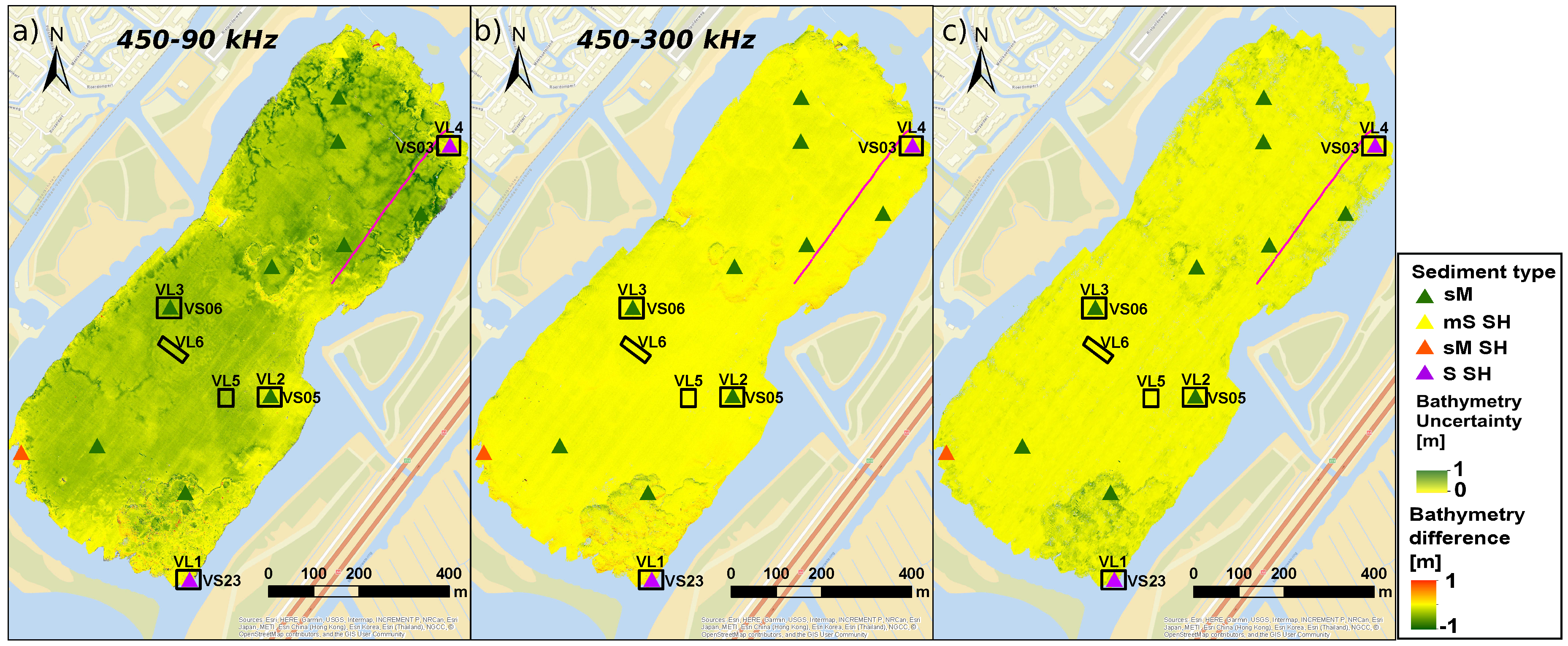
Table 1.
Survey parameters using an R2 Sonic 2026.
| Vlietland Lake | Port of Rotterdam | |
|---|---|---|
| Center frequency | 90, 100, 200, 300, 450 kHz | 90, 170, 255, 340, 425 kHz |
| Nominal pulse length | 150 s | 150 s |
| Number of beams | 256 | 256 |
| Beam width | , , , , | , , , , |
| Swath coverage | −65/ 65 | −65/ 65 |
| Beam spacing | equiangular | equiangular |
| Pulse-type | shaped continuous wave | shaped continuous wave |
Table 2.
Input parameters for the layered backscatter (BS) model and the bottom detection model. Layer 0 represents the water column, Layer 1 the surficial sediment, and Layer 2 the buried sediment.
Table 2.
Input parameters for the layered backscatter (BS) model and the bottom detection model. Layer 0 represents the water column, Layer 1 the surficial sediment, and Layer 2 the buried sediment.
| Variable | Unit | Layer 0 | Layer 1 | Layer 2 |
|---|---|---|---|---|
| Folks class | - | Fresh water | C/sM | sG |
| - | 9/6 | −1 | ||
| c | m/s | 1479 | 1449/1460 | 1977 |
| 1000 | 1145/1149 | 2492 | ||
| dB/m | 2.5 × 10 | 4.9/12.6 | 41.0 | |
| dB/m | 6.3 × 10 | 24.3/62.9 | 205.0 | |
| - | - | 1 × 10/1 × 10 | 2 × 10 | |
| - | - | 3.25/3.25 | 3.25 | |
| - | 5.17 × 10/5.17 × 10 | 1.29 × 10 | ||
| m | 20 [h] | 0.2. and 0.5 [d] | Semi-infinite |
Table 3.
Input parameters for the bottom detection model.
| Variable | Value |
|---|---|
| f | 90 kHz and 450 kHz |
| 150 s | |
| Pa | |
| m | |
| M | 256 |
Table 4.
Categorization of ground truth locations into subsets based on sediment properties, BS level, and measured bathymetry difference.
Table 4.
Categorization of ground truth locations into subsets based on sediment properties, BS level, and measured bathymetry difference.
| Subsets | Sediment | BS Level | Bathymetry Difference |
|---|---|---|---|
| A | Very coarse (sand with shells) | High | Negligible |
| B | Coarse (sand/mud mix with shells) | Intermediate | Negligible to low |
| C | Fine(sandy mud) | Low | Negligible |
| D | Fine (sandy mud) | Intermediate to very high | Significant |
© 2019 by the authors. Licensee MDPI, Basel, Switzerland. This article is an open access article distributed under the terms and conditions of the Creative Commons Attribution (CC BY) license (http://creativecommons.org/licenses/by/4.0/).
Share and Cite
MDPI and ACS Style
Gaida, T.C.; Mohammadloo, T.H.; Snellen, M.; Simons, D.G. Mapping the Seabed and Shallow Subsurface with Multi-Frequency Multibeam Echosounders. Remote Sens. 2020, 12, 52. https://doi.org/10.3390/rs12010052
AMA Style
Gaida TC, Mohammadloo TH, Snellen M, Simons DG. Mapping the Seabed and Shallow Subsurface with Multi-Frequency Multibeam Echosounders. Remote Sensing. 2020; 12(1):52. https://doi.org/10.3390/rs12010052
Chicago/Turabian StyleGaida, Timo C., Tannaz H. Mohammadloo, Mirjam Snellen, and Dick G. Simons. 2020. "Mapping the Seabed and Shallow Subsurface with Multi-Frequency Multibeam Echosounders" Remote Sensing 12, no. 1: 52. https://doi.org/10.3390/rs12010052
Note that from the first issue of 2016, this journal uses article numbers instead of page numbers. See further details here.