Geometric Processing and Accuracy Verification of Zhuhai-1 Hyperspectral Satellites


1
School of Remote Sensing and Information Engineering, Wuhan University, Wuhan 430079, China
2
State Key Laboratory of Information Engineering in Surveying, Mapping and Remote Sensing, Wuhan University, Wuhan 430079, China
*
Author to whom correspondence should be addressed.
Remote Sens. 2019, 11(9), 996; https://doi.org/10.3390/rs11090996
Submission received: 2 April 2019
/
Revised: 22 April 2019
/
Accepted: 23 April 2019
/
Published: 26 April 2019
Abstract
:The second batch of Zhuhai-1 microsatellites was successfully launched on 26 April 2018. The batch included four Orbita hyperspectral satellites (referred to as OHS-A, OHS-B, OHS-C, and OHS-D) and one video satellite (OVS-2A), which have excellent hyperspectral data acquisition abilities. For the first time in China, a number of hyperspectral satellite networks have been realized. To ensure the application of hyperspectral remote sensing data, a series of on-orbit geometry processing and accuracy verification studies has been carried out on the “Zhuhai-1” hyperspectral camera since the satellite was launched. This paper presents the geometric processing methods involved in the production of Zhuhai-1 hyperspectral satellite basic products, including geometric calibration and basic product production algorithms. The OHS images were used to perform on-orbit geometric calibration, and the calibration accuracy was better than 0.5 pixels. The registration accuracy of the image spectrum of the basic product after calibration, the single orientation accuracy, and the accuracy of the regional network adjustment were evaluated. The spectral registration accuracy of the OHS basic products is 0.3–0.5 pixels, which is equivalent to the spectral band calibration accuracy. The single orientation accuracy is better than 1.5 pixels and the regional network adjustment accuracy is better than 1.2 pixels. The generated area orthoimages meet the seamless edge requirements, which verifies that the OHS basic product image has good regional mapping capabilities and can meet the application requirements.

1. Introduction
Orbita is deploying the “Zhuhai-1” remote sensing micro-nanosatellite constellation, which will consist of 34 video, hyperspectral, radar, and infrared satellites distributed in different orbits [1]. The first batch of video satellites (OVS-1A, 1B) of the “Zhuhai-1” micro-nano constellation was launched successfully on 15 June 2017 and they have been in orbit for 1.5 years [2]. The second batch of satellites of the "Zhuhai-1" micro-nano constellation was successfully launched on 26 April 2018. The batch of satellites includes four Orbita hyperspectral satellites (OHS-A, OHS-B, OHS-C, and OHS-D) and one video satellite (OVS-2A), which have strong hyperspectral data acquisition abilities. A network of hyperspectral satellites has been realized in China for the first time [1]. Among them, four hyperspectral satellites have the same hardware configuration and operating status, and the cameras on each satellite are stitched together by three Complementary Metal Oxide Semiconductors (CMOS) sensors, with specific stitching on the focal surface, as shown in Figure 1.
Figure 2 shows the spectrum structure for each CMOS sensor. Each piece of the CMOS contains 5056 × 2968 pixels, and the imaging spectrum ranges from 400 to 1000 nm. In each CMOS sensor, the spectral average of 400–1000 nm is divided into 32 spectral segments through a filter, and each spectral segment occupies ≤ 2968/32 = 92 rows on the sensor. Only eight rows are used for 8-level integral imaging. The hyperspectral satellite camera can acquire images with a 10-m resolution, 150-km width, and 32 spectrum segments. The single-start continuous sweeping work time is no less than 2 min and the one-track working time is no more than 8 min, with a global coverage ability within 5 days.
The hyperspectral satellite platform is equipped with Global Navigation Satellite System (GNSS) receivers (supporting global positioning system (GPS) and Beidou) for measuring and downlinking the satellite position and speed. The satellite platform is equipped with three sensors and two sets of three-axis fiber optic gyroscopes. During the imaging stage, two sensors were used to observe the satellite attitude and the inertial attitude quaternion, processed by the sensor and gyro-Kalman filter, was transmitted to the ground station. The downlink frequency of the on-board GNSS and attitude data is 1 Hz. The main parameters of the four hyperspectral satellites are shown in Table 1.
This paper presents the geometric processing methods involved in the production of Zhuhai-1 hyperspectral satellite basic products, including geometric calibration and basic product production algorithms. In the experiments, the OHS was geometrically calibrated and the spectral segment registration, single-view orientation, and regional adjustment accuracy of the basic products were evaluated. The results show that the geometric calibration accuracy of the Zhuhai-1 hyperspectral satellite is better than 0.5 pixels. The registration accuracy of the spectrum of the basic product is 0.3–0.5 pixels, the accuracy of the basic product image is better than 1.5 pixels, and the accuracy of the regional network adjustment is better than 1.2 pixels. The basic product has the ability to form large areas and can meet the application requirements.
2. Methods
2.1. Geometric Calibration
Although the OHS payload is a planar CMOS payload, the imaging principle of each spectral segment of the OHS conforms to that of linear array push-broom imaging. The imaging geometric positioning model can be expressed as follows [3,4,5,6,7,8,9,10,11]:
In the above collinearity equation, represents the ground coordinates of the point in the World Geodetic System 1984 (WGS84) geocentric coordinate system and indicates the position of the OHS with respect to the WGS84 geocentric coordinate system. Furthermore, m denotes the scaling factor, denotes the rotation matrix for converting the coordinate system A to coordinate system B, is the principal point position, is the focal length, denotes the interior distortion effects, and is the offset matrix.
The OHS geometric calibration model mainly considers the compensation of the load installation error, attitude and orbit system error, and camera distortion. The orbit system error and attitude system error are equivalent and can be compensated for via unified modeling [6,7,8,9]. The load installation error has the same influence on geometric positioning as the attitude system error; hence, it can also be equivalent to the attitude system error. Therefore, the offset matrix shown in Equation (1) can be used to compensate for the attitude system error, and the influence of the load installation error and attitude and orbit system error on geometric positioning can be eliminated simultaneously. is defined as follows:
For camera distortion, the OHS single-band uses several lines in the CMOS array to simulate time delay integration (TDI) Charge-coupled Device (CCD) push-broom; hence, the distortion model of the single-band can incorporate the directional angle model shown in Equation (3) [12,13,14,15]:
where s is the image column. Therefore, the geometric calibration model of the OHS single spectral band is shown in Equation (4):
Considering the strong correlation between and ,, the geometric calibration can be completed by using the iterative solution of and , parameters so that the geometric calibration can be completed when the number of geometric control points of a single spectral segment is no less than .
As shown in Figure 2, the OHS camera has 32 spectral segments, which need to be geometrically calibrated. Since the spectral responses of the 32 spectral segments are quite different, if the control points are obtained by matching each spectral segment with the Digital Orthophoto Map (DOM) of the calibration field before geometric calibration, the calibration accuracy of each spectral segment will be inconsistent due to the difference in control accuracy. Considering that the imaging time interval of the adjacent spectral segments is short and the difference in the spectral response is relatively small, the registration accuracy between adjacent spectral segments will be higher than the accuracy between spectral segments and the DOM. Therefore, this paper proposes a recursive geometric calibration method for adjacent spectral segments to complete the geometric calibration of all spectral segments. The process involves the following steps:
- (1).
- Using the DOM of the calibration field as a reference, select the spectral segment that is closest to the radiating characteristics of the DOM image as the starting spectral segment (assuming this is spectral segment N), use a high-precision matching algorithm to match N and DOM, obtain control points, and determine and , of N using Equation (4);
- (2).
- According to the calibration parameters solved in step (1), construct the geometric positioning model of N using Equation (4);
- (3).
- Register spectral segment N-1 and spectral segment N to obtain the corresponding points , and calculate the ground coordinates corresponding to the image points according to the geometric positioning model of N constructed in step (2). Taking as the geometric control point of N-1, the offset matrix of N-1 is the same as that of N in step 1). Solve for , of N-1 using Equation (4) and update the geometric positioning model of N-1;
- (4).
- Repeat step (3) until the geometric calibration of spectral segment 1 is completed;
- (5).
- For spectral segment N+1 to 32, follow steps (3) to (4) to recursively complete the geometric calibration.
2.2. Production
Orbita has considered both the amount of image data and the practical application requirements. The basic products released to the outside world are the 32-band registration image products of the single CMOS, and the regional mosaic image is used as a value-added product. Therefore, although the single imaging width of the hyperspectral satellite can reach 150 km, the width of the basic product released by the company is 50 km. OHS basic product processing is mainly performed for 32-band registration and Rational Function Coefficients (RPC) generation.
The essence of spectral registration is to determine the correspondence of homonymous points between different spectral segments. Figure 3 shows a schematic of a synonymous point with four spectral segments as examples. As shown, any imaging point on B1 can be used to determine the location of homonymous image points on B2, B3, and B4 based on the principle that homonymous points should be located at the same position on the ground (positioning consistency constraint). The accuracy of the corresponding relationship is mainly limited by the accuracy of the geometric positioning parameters, including the accuracy of the attitude and orbit used in positioning, the accuracy of orientation elements in the camera, and the accuracy of the elevation data.
Geometric calibration accurately restored the camera’s interior orientation elements and determined the exact position relationship of the 32 spectral segments on the focal plane. Therefore, the influence of the interior orientation element error on the determination of homonymous points can be ignored. For elevation fluctuation caused by stereoscopic parallax, the maximum difference in the view angle between the OHS spectrum (band 1 and band 32) is less than 3°, considering geometric positioning in the global 90 m grid SRTM as elevation data, an elevation accuracy of 16 m, and the effect of stereoscopic parallax for identical point determination being less than 0.1 pixels, which can be neglected. For attitude and orbit measurement errors, the imaging time interval between adjacent spectral segments for identical objects is less than 0.1 s, while the attitude and orbit measurement errors over a short period are mainly systematic errors, which do not affect the accuracy of the identical point relationship determination. Therefore, the registration of OHS spectral segments can be realized based on the consistency constraint of homonymous point location. The algorithm is as follows:
- (6).
- Using the geometric calibration results, establish a geometric positioning model for each spectral segment of the OHS according to Equation (4);
- (7).
- Select the intermediate spectral segment as the reference spectral segment (such as the 15th spectral segment), which has an image size of . Based on the spectral segment geometric positioning model established in (1), the terrain-independent method is used to generate the RPC parameters of the spectral segment;
- (8).
- For any of the spectral segments N (N≠15), generate a new image of size as follows:
- (a)
- For any image point on the image, calculate the ground coordinate corresponding to using the geometric positioning model of the reference spectral segment;
- (b)
- Calculate corresponding to the image point coordinate in spectral segment N by using the positioning model of N;
- (c)
- Calculate the gray value at using the linear interpolation method and assign to the new image;
- (d)
- Repeat steps (a)–(c) until all pixels of the new image have been calculated.
- (9).
- Repeat step (3) until all segments have been resampled.
3. Results and Discussion
3.1. Study Areas and Data Sources
Geometric calibration is the premise of high data quality and the basis for satellite on-orbit processing. The OHS image of the Hubei area (No. 2018-09-28-OHS-Hubei) obtained on 28 September 2018, was used for OHS geometric calibration. The image size was 15,168 (5056 × 3) × 8147 pixels. As shown in Table 2, the calibration control data include DOM and Digital Elevation Model (DEM) data in the Hubei area. The DOM resolution of the Hubei area is 2 m, the plane precision is better than 4 m, the DEM resolution is 15 m, and the elevation accuracy is better than 5 m (1). The average elevation of the area is 264 m and the maximum height difference is 556 m. Thumbnails of the image and control data are shown in Figure 4.
To fully verify the accuracy of the basic products after OHS geometric calibration, the spectral segment registration, single-view orientation, and regional adjustment accuracy of the product were evaluated. Three scene images obtained on 12 September 2018, 5 August 2018, and 10 October 2018, in Beijing, Tianjin, and Shandong, respectively, were used for accuracy evaluation of the spectral band registration. For the single-view orientation accuracy assessment, images obtained on 13 January 2019 and 17 January 2019 were collected. Also, three scene images obtained on 24 January 2019 are shown from Inner Mongolia, Henan and Hebei, respectively. DOM and DEM data were used for verification control of the corresponding area. The DOM resolution is 2 m, the plane precision is 5 m, the DEM resolution is 15 m, and the elevation accuracy is 3 m. Thumbnails of the experimental data and control data are shown in Figure 5, Figure 6, and Figure 7 for the different areas. Four-track 221-view basic product images covering Shanxi (12 August 2018, 21 January 2011, 7 September 2018, and 19 November 2018) were collected for regional adjustment accuracy assessment. The details of the calibration and verification data are shown in Table 2.
3.2. Geometric Calibration
The 15th band is selected as the reference, and the 2018-09-28-OHS-Hubei image and Hubei DOM image are matched using the automatic matching algorithm [16]. To reduce the influence of the random error of the attitude and orbit measurements on the geometric calibration, only 2102 matching control points are used for geometric calibration from 4000 to 6000 lines in the 2018-09-28-OHS-Hubei image. The distribution is shown in Figure 8.
Since the offset matrix mainly eliminates satellite attitude and orbit measurement system error, the camera creates system error, which cannot eliminate the internal orientation element error. Therefore, the positioning error after solving the offset matrix mainly reflects the internal orientation element error (camera distortion, etc.). As shown in Table 1 and Figure 9a, due to satellite orbit focusing, band reconstruction, etc., the on-board real camera parameters vary significantly from the pre-launch laboratory measurement parameters. As shown in Table 3, the positioning error is still 36 pixels (about 360 m) after solving the offset matrix, but after further solving the camera distortion parameters, the positioning accuracy is increased to 0.5 pixels (5 m), which is equivalent to the control precision.
The remaining 31 spectral bands are geometrically scaled using the 15th spectral band after calibration as the reference spectral band. The calibration results are shown in Figure 10. It can be seen that the calibration accuracy of each spectrum band is 0.3–0.4 pixels.
3.3. Band-to-Band Registration Accuracy
The registration accuracy of adjacent spectral segments was verified by using 2018-9-12-OHS-Beijing, 2018-8-5-OHS-Tianjing, and 2018-10-10-OHS-Shandong images. A high-precision matching algorithm [16] is used to extract the same-named points from the adjacent spectral segments of the above basic products, and the spectral segment registration accuracy is evaluated by calculating and counting the coordinate deviations of the same-named image points of the adjacent spectral segments [4]. The results are shown in Figure 11.
As can be seen from Figure 11, the spectral registration accuracy of the evaluation of the three-field experimental data is 0.3 to 0.5 pixels. As mentioned above, this study uses the method of positioning consistency constraints for spectral segment registration. The registration accuracy mainly depends on the elevation error, attitude and orbit error, and internal orientation element error. Among them, the influence of the global 90 m SRTM elevation data on spectral segment registration is less than 0.1 pixels. In addition, the imaging interval of adjacent spectral bands is only within 0.1 s, the attitude error is mainly systematic error, and the influence on spectral segment registration can be neglected. The accuracy of spectral segment registration depends mainly on the accuracy of spectral band calibration. A comparison of the results shown in Figure 10 and Figure 11 shows that the accuracy of the spectral alignment in the evaluation is comparable to the calibration accuracy between the spectral bands. Finally, the overlay display effect of the spectrum segment of OHS basic products is shown in Figure 12.
3.4. Interior Orientation Determination Accuracy Evaluation
To verify the intra-image accuracy of the OHS basic product, the artificial puncture method was used to obtain control points from three scene images of 2019-01-13-OHS-Neimeng, 2019-01-17-OHS-Henan, and 2019-01-17-OHS-Hebei. The control points are 33, 33, and 31, as shown in Figure 13.
The positioning accuracies of all the images were evaluated based on the geometric control points (GCPs), where an image affine model based on the RPC defined by Equation (5) is used as the exterior orientation model [17,18,19].
The image-based affine model based on RPC can eliminate the error of the attitude and orbit system. The accuracy after adjusting the control point mainly depends on the random error of the attitude and orbit. Because the accuracy of orbit determination is high, the accuracy shown in Table 4 mainly depends on the attitude random error, including errors caused by attitude measurement random error and platform stability. According to Table 1, the random error of the attitude measurement is 15″ (3) and the geometric positioning error is 1.2 pixels (1). In fact, because the imaging time of the OHS basic product standard scene is only 7 s, which is very short, and the attitude measurement error in the time is mainly systematic, the random error may be less than 15″ (3) and the resulting positioning error should be less than 1.2 pixels. Considering the fact that the attitude downlink frequency is only 1 Hz, under the condition that the attitude angular velocity is constant within 1 s, the attitude of the arbitrary imaging time is interpolated based on the measurement attitude of the adjacent 1 s during ground processing. However, since the stability of the OHS platform is only 0.002°/s (1), the angular velocity of the attitude within 1 s is not constant; hence, the random error caused by the stability of the platform does not exceed 0.002°, and the geometric positioning error does not exceed 1.7 pixels (1). In summary, the effect of the attitude random error on the internal accuracy should theoretically not exceed 2 pixels. Table 4 shows that the orientation accuracy of the three basic products is better than 1.5 pixels, and Figure 14 shows the positioning residuals are random, which is consistent with the theoretical concept of “not exceeding 2 pixels”.
3.5. Results of Block Adjustment
Data for Shanxi were collected in this experiment. The detailed information is shown in Table 2. The 221 scenes of the basic product image, image distribution position, and matching connection point distribution are shown in Figure 15.
Using the high-precision matching algorithm [16], 13,086 connection points were obtained on the 221-scene image. Based on the image affine model of RPC expressed in Equation (5), DEM-assisted uncontrolled plane adjustment [20,21,22] was performed on the region 221-scene image. The auxiliary DEM is the DEM with a 25 m resolution and 5 m elevation accuracy of the Shanxi region. The results are shown in the table below.
The adjustment accuracy in Table 5 depends on the elevation influence and the accuracy within the image. As can be seen from Table 2, the maximum intersection condition of the 221 scene data is 9.82° and −8.69°, and the elevation effect in plane adjustment is 0.2 pixels, which is basically negligible. Therefore, the adjustment accuracy of 1.15 pixels in this area mainly reflects the accuracy of the image, which is consistent with the above theoretical concept of “not exceeding 2 pixels.” Further, an orthophoto image of the region was generated, and the result is shown in Figure 16. The result satisfies the accuracy requirement of 1 pixel of the image mosaic edge and verifies that the OHS basic product image has a large area mapping capability. A detailed image of the local edge joint is shown in Figure 17 and Figure 18.
4. Conclusions
Based on the characteristics of the Zhuhai-1 hyperspectral satellite, this paper proposes a hyperspectral image geometric calibration model method and a basic product production method. The OHS image was used to perform on-orbit geometric calibration, and the spectral registration accuracy, single-view orientation accuracy, and regional network adjustment accuracy of the basic product spectrum after calibration were evaluated. The experimental results show that the spectral alignment accuracy of the OHS basic products is 0.3–0.5 pixels, which is equivalent to the spectral segment calibration accuracy. The single-view orientation accuracy should theoretically be “no more than 2 pixels.” The accuracy of the actual evaluation result is better than 1.5 pixels (0.8–1.5 pixels (1) and the regional network adjustment accuracy is better than 1.2 pixels (1). The generated area orthophoto image satisfies the seamless edge requirement. It is verified that the image of OHS basic products can perform regional mapping and meet the application requirements.
Author Contributions
Y.J. and J.W. conceived and designed the experiments; Y.J. and J.W. performed the experiments; G.Z., L.Z., X.L., and J.W. analyzed the data; Y.J. and J.W. wrote the paper; and all authors edited the paper.
Funding
This research was funded by the Key Research and Development Program of the Ministry of Science and Technology (grant number 2016YFB0500801), the National Natural Science Foundation of China (grant numbers 91538106, 41501503, 41601490, and 41501383) and the Open Foundation of Key Laboratory of Precise Engineering and the Industry Surveying of National Administration of Surveying, Mapping and Geoinformation (grant number PF2017-4).
Acknowledgments
We thank the research team at Orbita for providing the OHS images. Furthermore, we would like to thank the reviewers for their helpful comments.
Conflicts of Interest
The authors declare no conflict of interest. The funding sponsors had no role in the design of the study; in the collection, analyses, or interpretation of data; in the writing of the manuscript; or in the decision to publish the results.
References
- Orbita. Orbita. Available online: https://www.myorbita.net/ (accessed on 1 March 2019).
- Zhan, H. The First Two Satellite OVS-1A/1B of Zhuhai-1 Remote-sensing Micro-nano Satellites Constellation Launched Successfully. Space Int. 2017, 462, 1674–9030. [Google Scholar]
- Tadono, T.; Shimada, M.; Murakami, H.; Takaku, J. Calibration of PRISM and AVNIR-2 onboard ALOS daichi. IEEE Trans. Geosci. Remote Sens. 2009, 47, 4042–4050. [Google Scholar] [CrossRef]
- Jiang, Y.H.; Guo, Z.; Tang, X.M.; Li, D.; Pan, H.B. Geometric Calibration and Accuracy Assessment of ZiYuan-3 Multispectral Images. IEEE Trans. Geosci. Remote Sens. 2014, 52, 4161–4172. [Google Scholar] [CrossRef]
- Furukawa, H.; Jeminous, M.; Cui, G.; Laks, H.; Sen, L. In-Flight CCD Distortion Calibration for Pushbroom Satellites Based on Subpixel Correlation. IEEE Trans. Geosci. Remote Sens. 2008, 46, 2675–2683. [Google Scholar] [Green Version]
- Radhadevi, P.V.; Solanki, S.S. In-flight geometric calibration of different cameras of IRS-P6 using a physical sensor model. Photogramm. Rec. 2010, 23, 69–89. [Google Scholar] [CrossRef]
- Bouillon, A.; Breton, E.; Lussy, F.D.; Gachet, R. SPOT5 geometric image quality. In Proceedings of the IEEE International Geoscience & Remote Sensing Symposium, Toulouse, France, 21–25 July 2003. [Google Scholar]
- Bouillon, A.; Breton, E.; Lussy, F.D.; Gachet, R. SPOT5 HRG and HRS first in-flight geometric quality results. In Proceedings of the International Symposium on Remote Sensing, Crete, Greece, 23–27 September 2002. [Google Scholar]
- Zhang, G.; Wang, J.; Jiang, Y.; Zhou, P.; Zhao, Y.; Xu, Y. On-Orbit Geometric Calibration and Validation of Luojia 1-01 Night-Light Satellite. Remote Sens. 2019, 11, 264. [Google Scholar] [CrossRef]
- Tang, X.; Zhang, G.; Zhu, X.; Pan, H.; Jiang, Y.; Zhou, P.; Wang, X. Triple Linear-array Imaging Geometry Model of Ziyuan-3 Surveying Satellite and Its Validation. Acta Geod. Cartogr. Sin. 2013, 4, 33–51. [Google Scholar]
- Tadono, T.; Shimada, M.; Hashimoto, T.; Takaku, J.; Mukaida, A.; Kawamoto, S. Results of calibration and validation of ALOS optical sensors, and their accuracy assesments. In Proceedings of the IEEE International Geoscience & Remote Sensing Symposium, Barcelona, Spain, 23–27 July 2007. [Google Scholar]
- Jiang, Y.; Zhang, G.; Li, D.; Tang, X.; Huang, W.; Li, L. Correction of Distortions in YG-12 High-Resolution Panchromatic Images. Photogramm. Eng. Remote Sens. 2015, 81, 25–36. [Google Scholar] [CrossRef]
- Yong-hua, J.; Guo, Z.; Xinming, T.; Deren, L.; Wen-chao, H. Detection and Correction of Relative Attitude Errors for ZY1-02C. IEEE Trans. Geosci. Remote Sens. 2014, 52, 7674–7683. [Google Scholar] [CrossRef]
- Jiang, Y.; Xu, K.; Zhao, R.; Zhang, G.; Cheng, K.; Zhou, P. Stitching images of dual-cameras onboard satellite. ISPRS J. Photogramm. Remote Sens. 2017, 128, 274–286. [Google Scholar] [CrossRef]
- Zhang, G.; Jiang, Y.; Li, D.; Huang, W.; Pan, H.; Tang, X.; Zhu, X. In-Orbit Geometric Calibration And Validation Of Zy-3 Linear Array Sensors. Photogramm. Rec. 2014, 29, 68–88. [Google Scholar] [CrossRef]
- Leprince, S.; Barbot, S.; Ayoub, F.; Avouac, J.-P. Automatic and Precise Orthorectification, Coregistration, and Subpixel Correlation of Satellite Images, Application to Ground Deformation Measurements. IEEE Trans. Geosci. Remote Sens. 2007, 45, 1529–1558. [Google Scholar] [CrossRef] [Green Version]
- Wang, T.; Guo, Z.; Jiang, Y.; Wang, S.; Huang, W.; Li, L. Combined Calibration Method Based on Rational Function Model for the Chinese GF-1 Wide-Field-of-View Imagery. Photogramm. Eng. Remote Sens. 2016, 82, 291–298. [Google Scholar] [CrossRef]
- Wang, T.; Zhang, G.; Yu, L.; Zhao, R.; Deng, M.; Xu, K. Multi-Mode GF-3 Satellite Image Geometric Accuracy Verification Using the RPC Model. Sensors 2017, 17, 2005. [Google Scholar] [CrossRef] [PubMed]
- Wang, T.; Guo, Z.; Li, D.; Zhao, R.; Deng, M.; Tong, Z.; Lei, Y. Planar block adjustment and orthorectification of Chinese spaceborne SAR YG-5 imagery based on RPC. Int. J. Remote Sens. 2018, 39, 640–654. [Google Scholar] [CrossRef]
- Pan, H.; Zou, Z.; Zhang, G.; Zhang, Y.; Wang, T. Block adjustment of high resolution satellite image using RFM with the same stripe constraint. Remote Sens. Land Resour. 2016, 28, 46–52. [Google Scholar]
- Liu, J.; Wang, D.H.; Zhang, Y.S.; Wang, H. Bundle Adjustment of Airborne Three Line Array Imagery Based on Unit Quaternion. Acta Geod. Cartogr. Sin. 2008, 37, 451–457. [Google Scholar]
- Beckett, K.; Rampersad, C.; Putih, R.; Robertson, B.; Steyn, J.; Tyc, G. RapidEye product quality assessment. Proc. SPIE Int. Soc. Opt. Eng. 2009, 7474. [Google Scholar] [CrossRef]
Figure 1.
Schematic of the focal plane arrangement of the hyperspectral camera.

Figure 2.
Schematic of the CMOS sensor spectrum distribution.
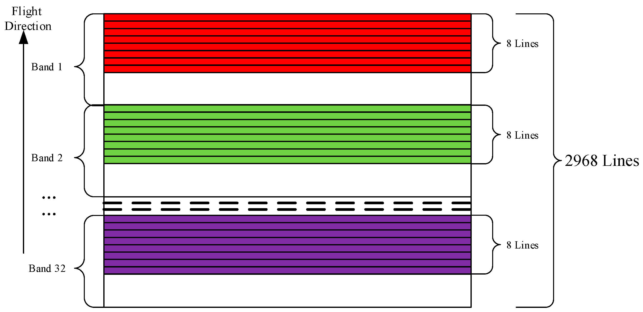
Figure 3.
Schematic of correspondence between homonymous points in different spectral segments.
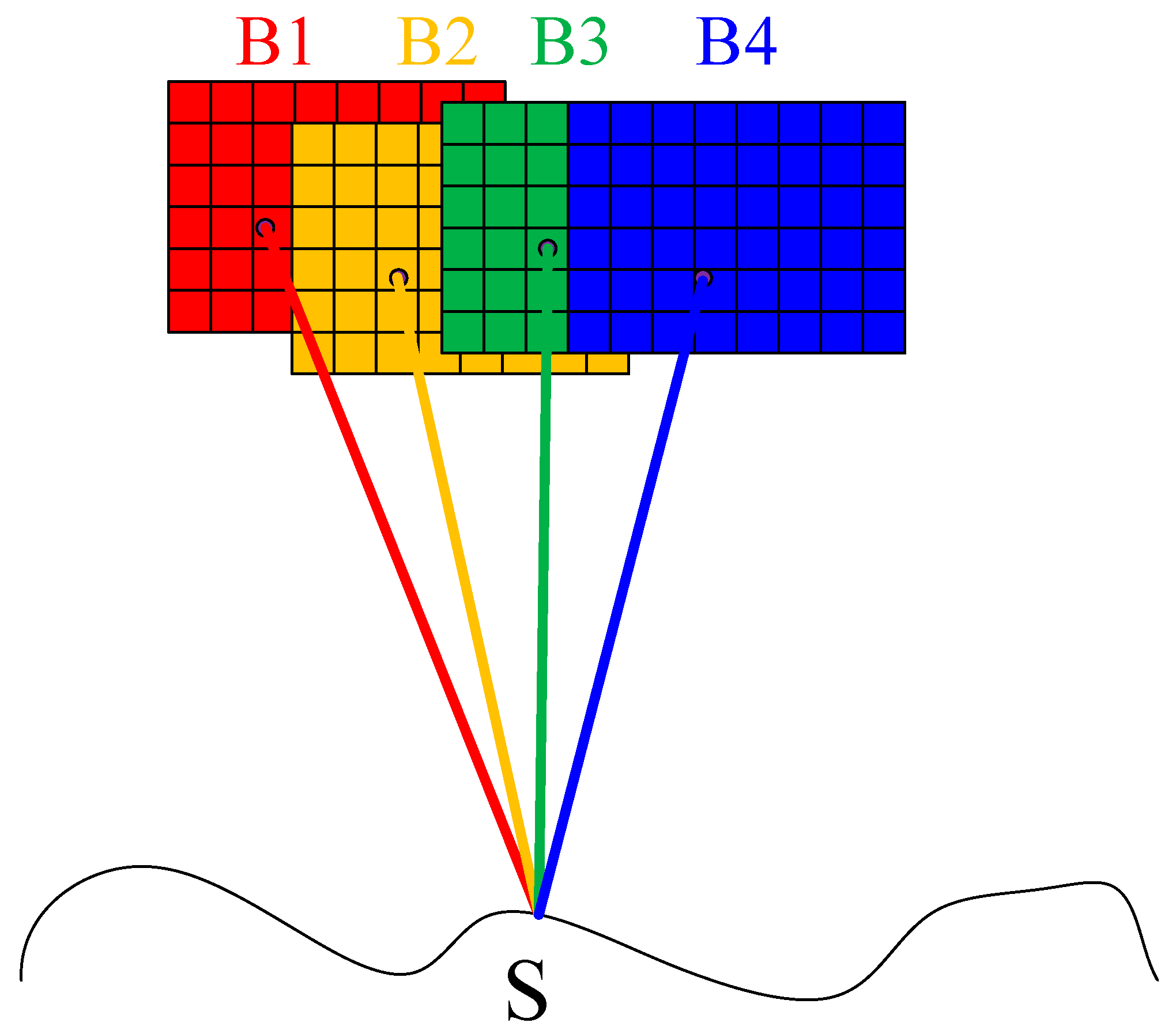
Figure 4.
Hubei regional geometric calibration image and control data.

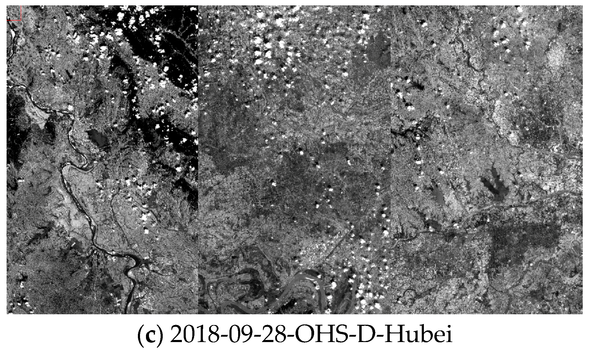
Figure 5.
Neimeng regional control and verification data.
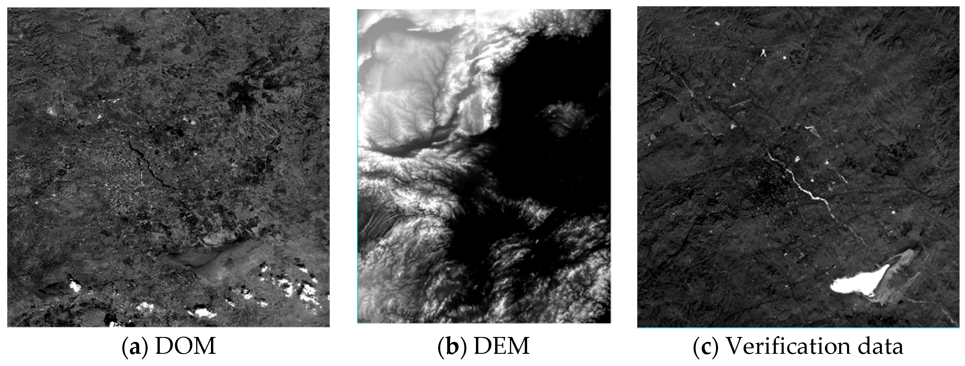
Figure 6.
Henan regional control and verification data.

Figure 7.
Hebei regional control and verification data.

Figure 8.
2018-09-28-OHS-Hubei image control point distribution (4000–6000 lines).
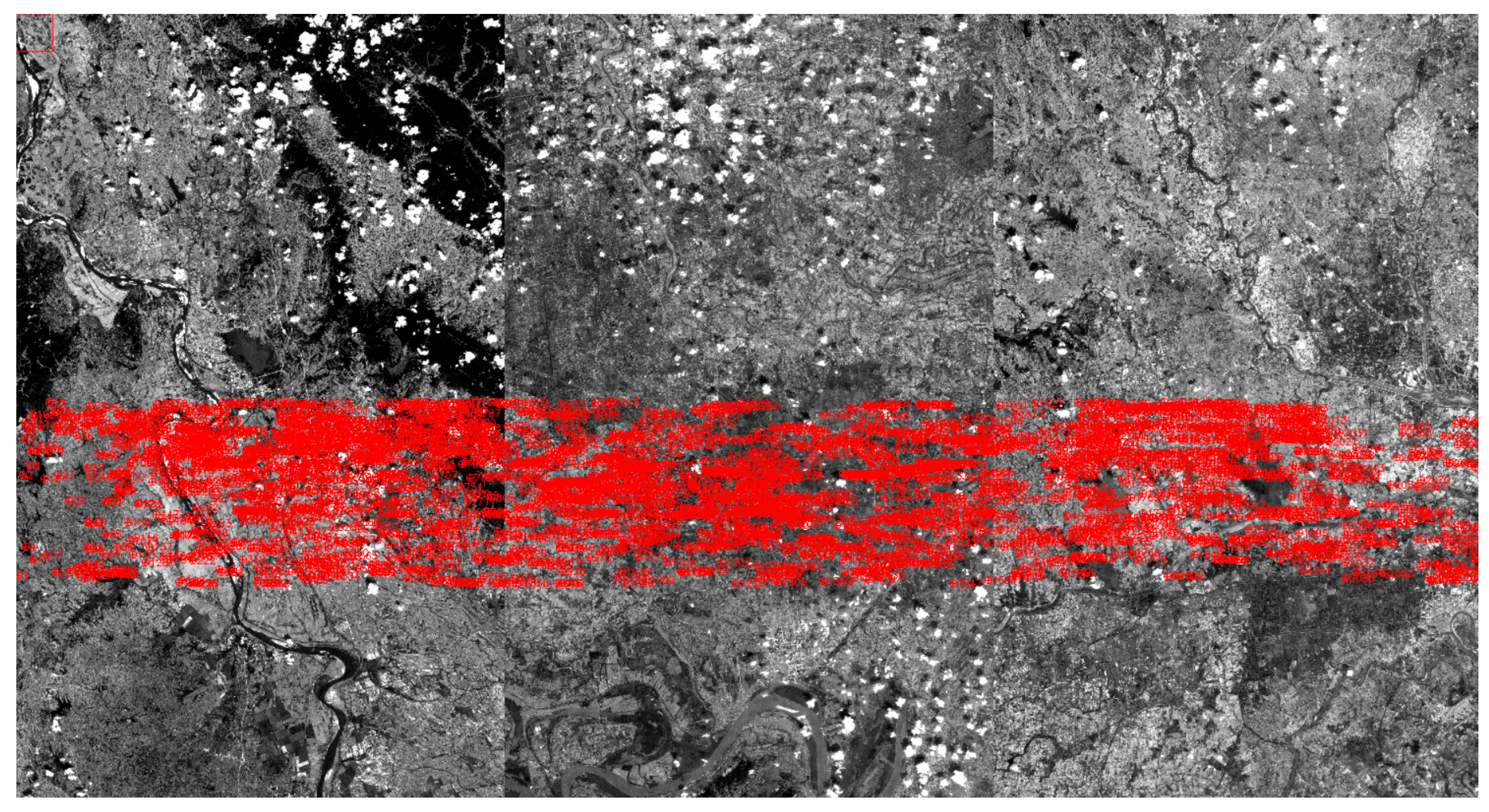
Figure 9.
2018-09-28-OHS-Hubei image calibration residual diagram.
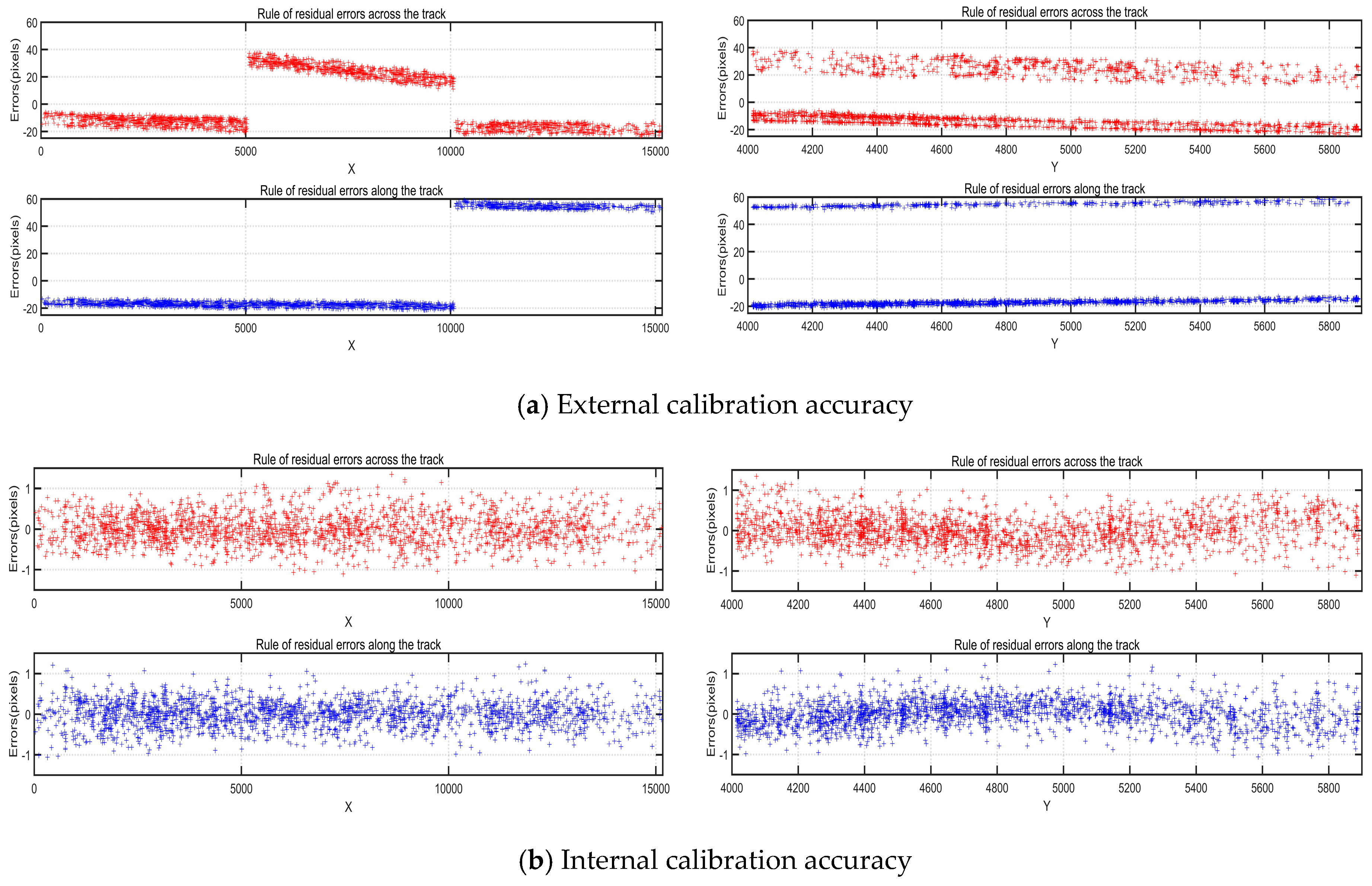
Figure 10.
Calibration accuracies of other spectral calibrations.

Figure 11.
Evaluation results of spectral segment registration accuracy.
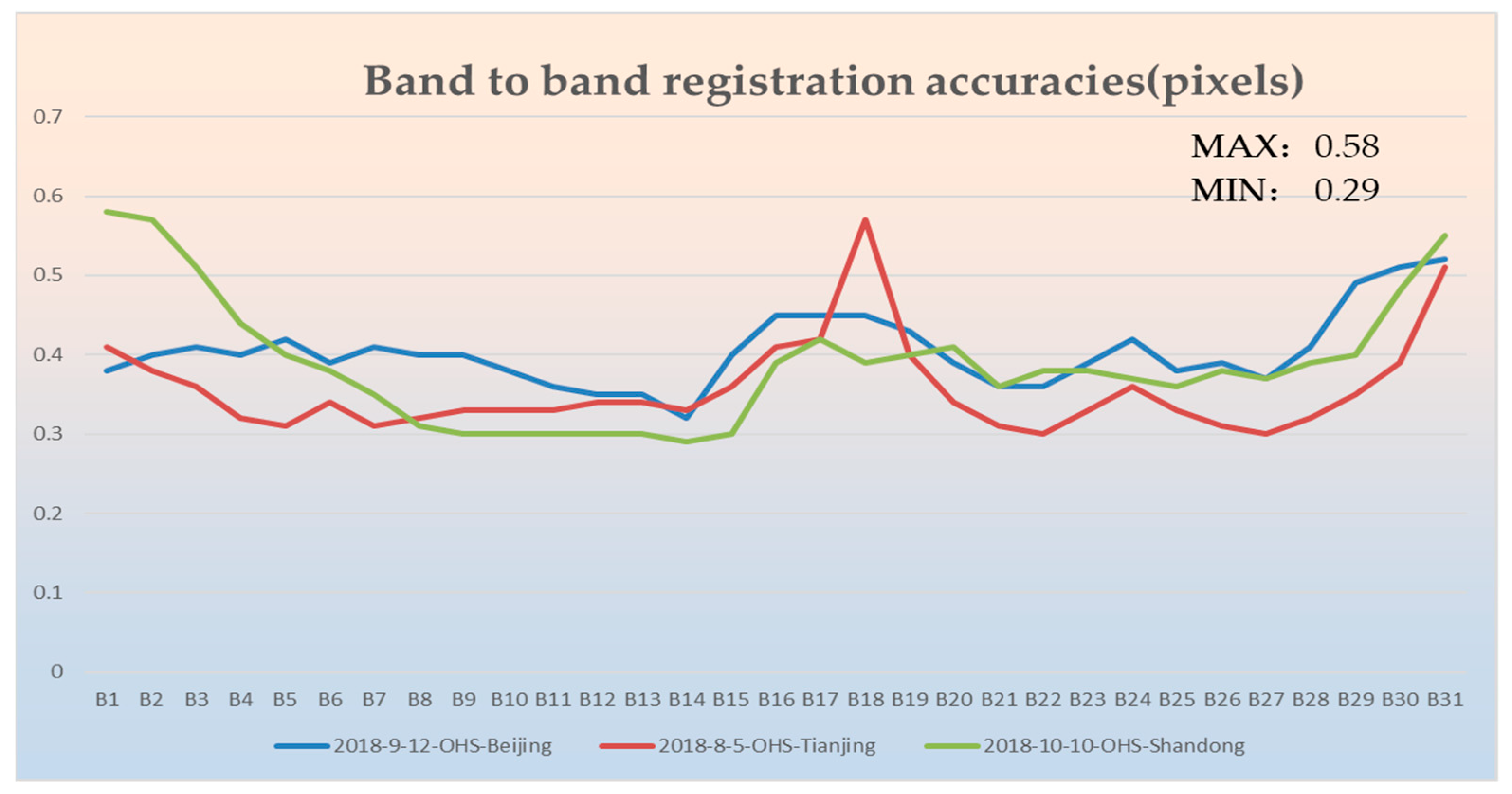
Figure 12.
Overlay display schematic map of different spectrum segments in Gansu Province.
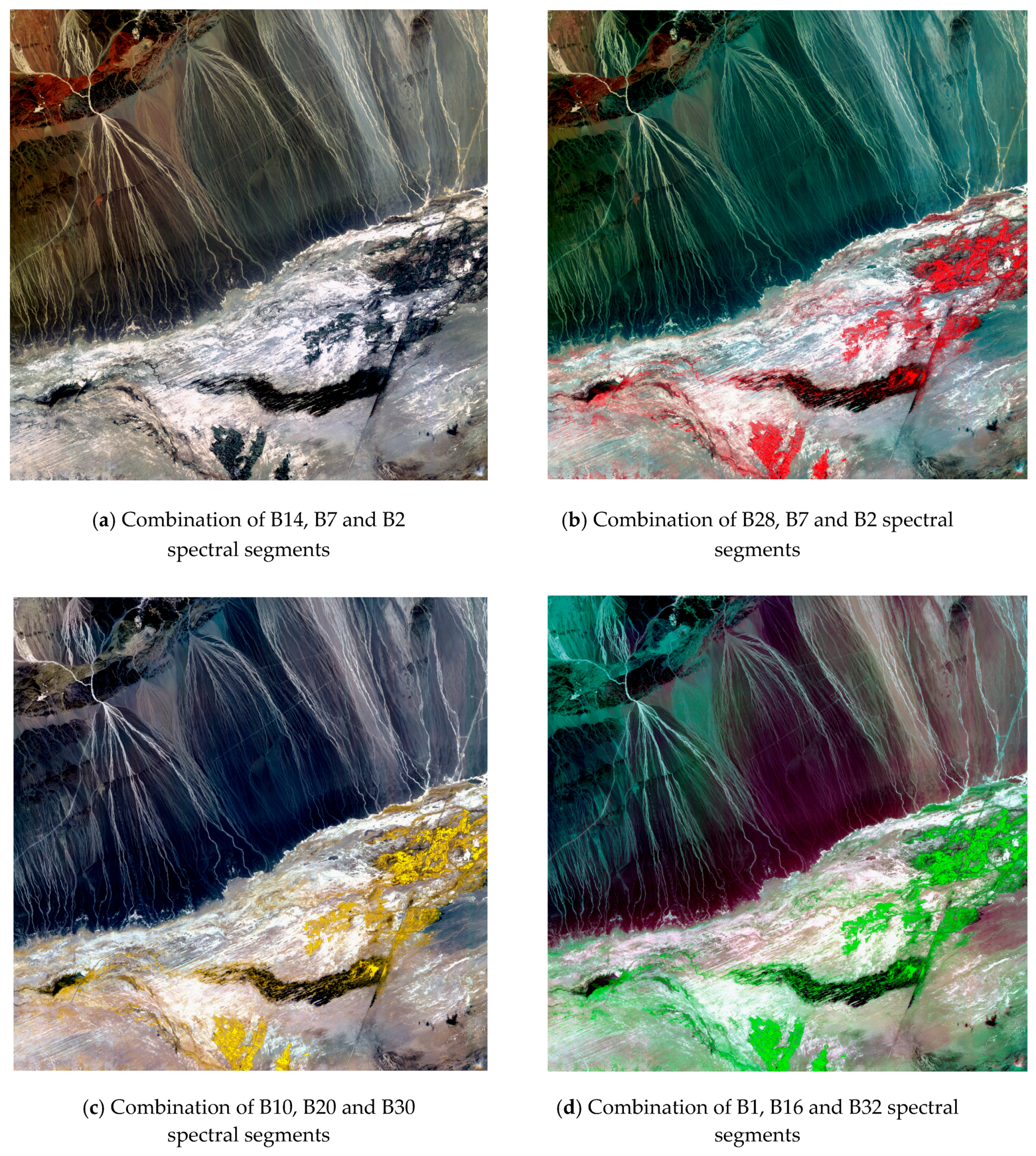
Figure 13.
Image control point distribution.

Figure 14.
Single scene directional residual diagram.
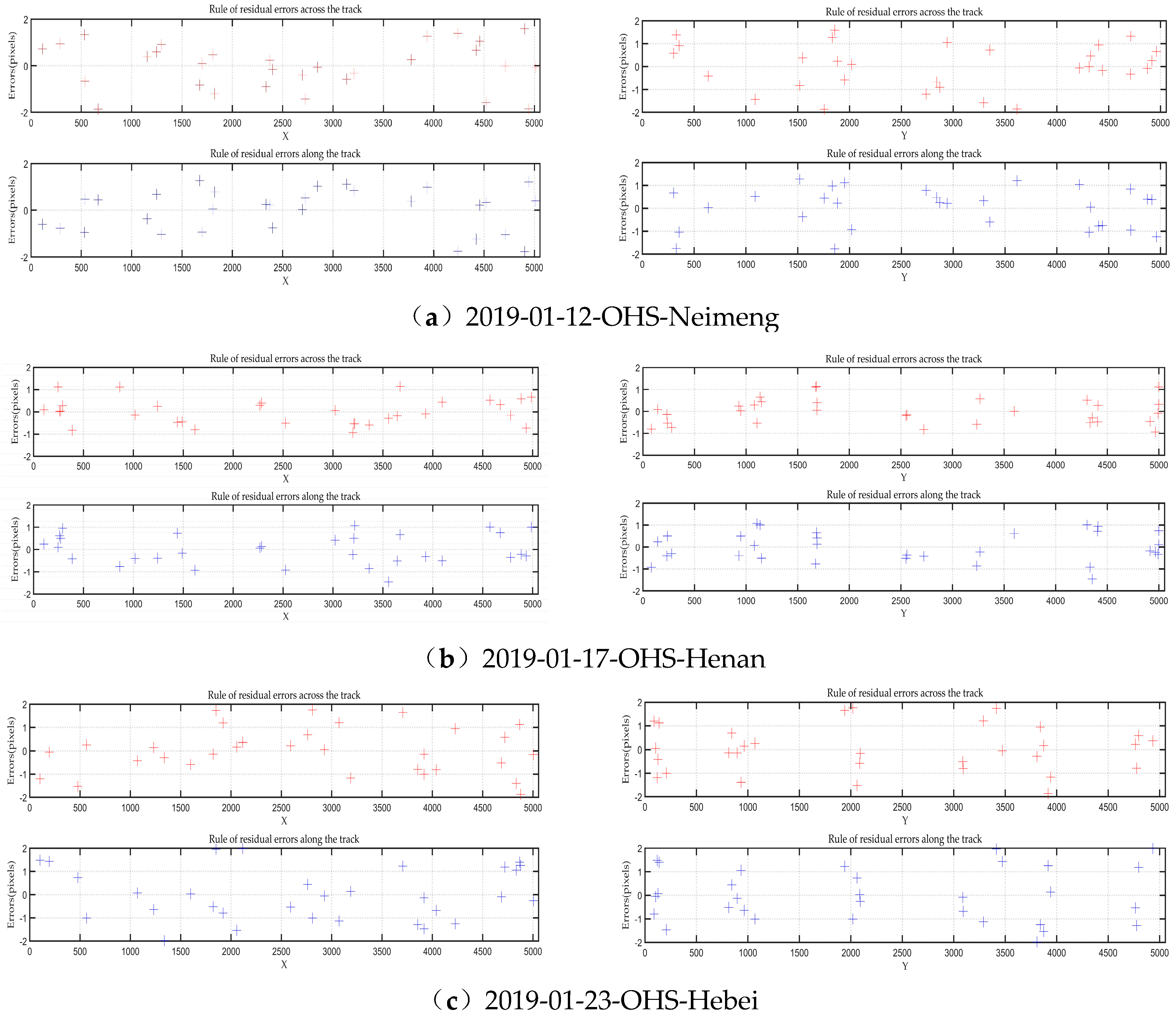
Figure 15.
Image and connection point distribution.
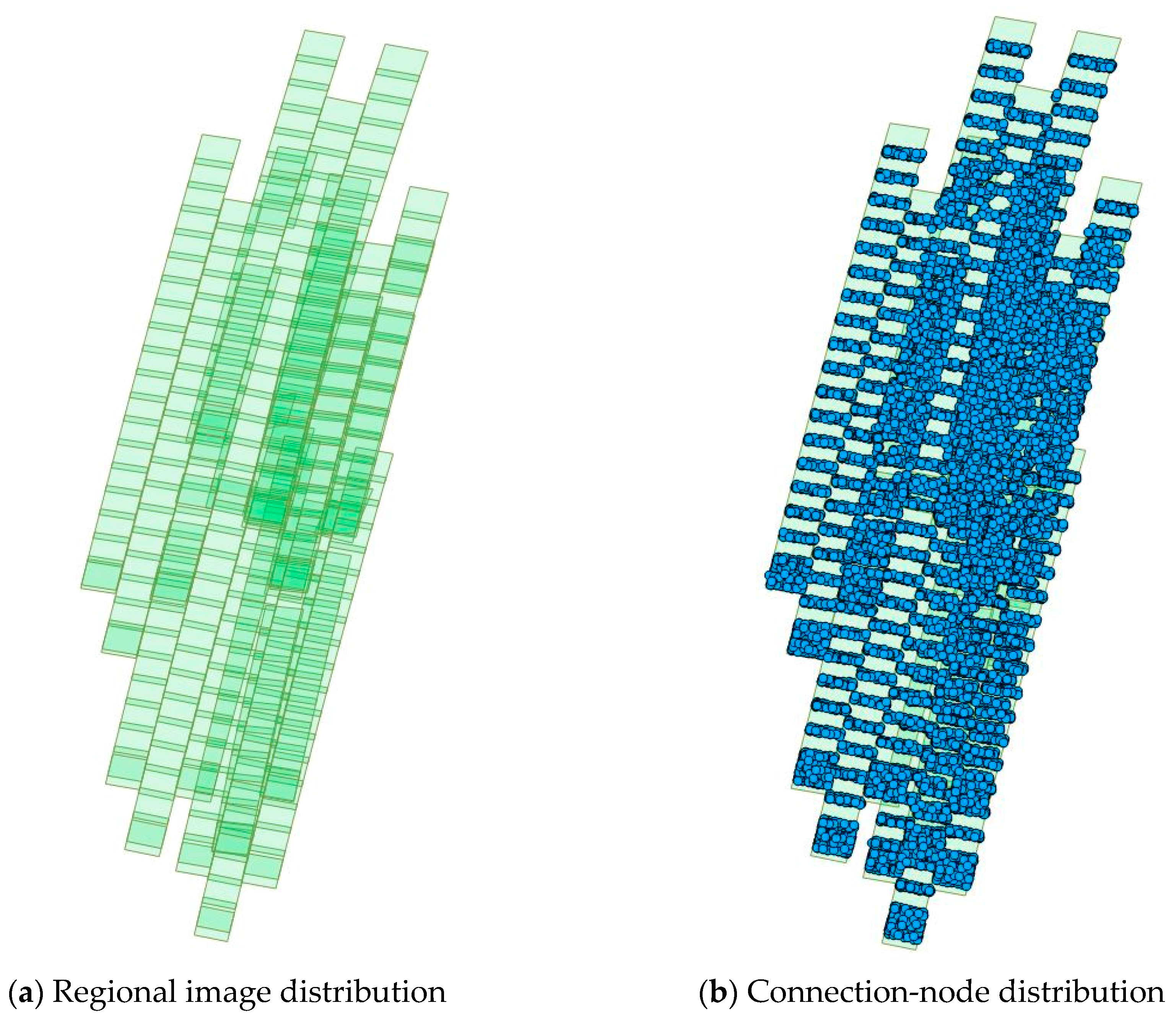
Figure 16.
Diagram of orthographic image overlay.
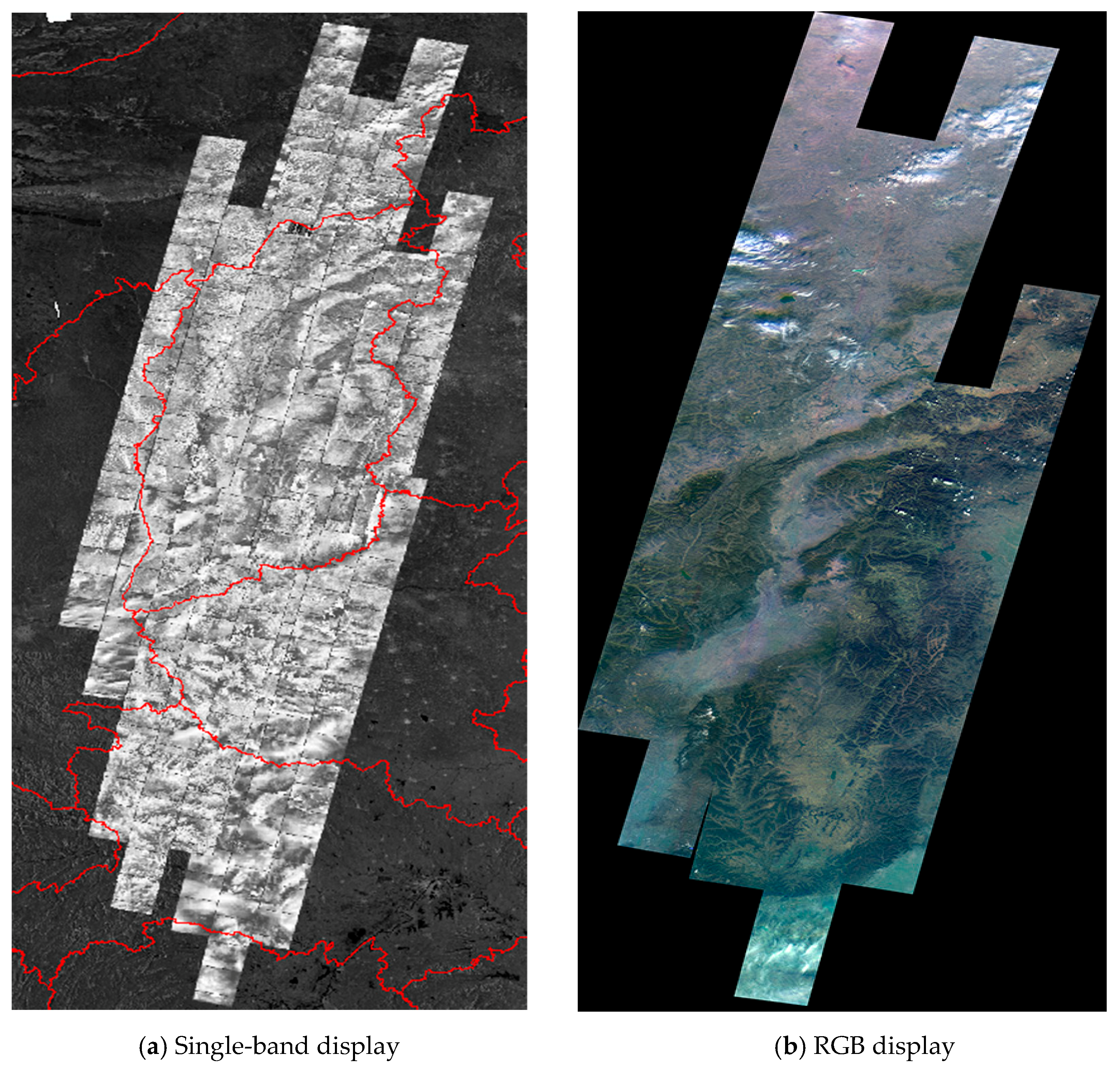
Figure 17.
Sketch of the left and right edge of the image.

Figure 18.
Sketch of the upper and lower edge of the image.


Table 1.
Orbita hyperspectral satellite (OHS) parameters.
| Satellite Platform | Total satellite mass | 67 kg |
| Orbit height | 500 km | |
| Orbit inclination angle | 98° | |
| Regression cycle | 5 days | |
| Global positioning system (GPS) positioning precision | 15 m | |
| Attitude accuracy | 15″ (3) | |
| Attitude maneuver | ±45°/80 s | |
| Attitude stability | 0.002°/s (1) | |
| Satellite Payload | Detector size | 4.4 µm |
| Field of view (FOV) | 20.5° | |
| Spectral range | 400–1000 nm | |
| Quantitative level | ≥12 bits | |
| Band number | 32 | |
| Signal Noise Ratio (SNR) | ≥300 dB | |
| Ground sample distance | 10 m | |
| Ground swath | 150 km |
Table 2.
Imaging information of experimental data.
| ID | Imaging Angle (°) | Imaging Time | Band | ||
|---|---|---|---|---|---|
| Roll | Pitch | Yaw | |||
| 3.2. Geometric Calibration | |||||
| 2018-09-28-OHS-Hubei | −1.09° | 0.00° | 3.18° | 2018-09-28 | 1-32 |
| 3.3. Band-to-Band Registration Accuracy | |||||
| 2018-9-12-OHS-Beijing | −5.26° | 0.00° | 2.81° | 2018-09-12 | 1-32 |
| 2018-8-5-OHS-Tianjing | −11.85° | 0.00° | 2.72° | 2018-08-05 | 1-32 |
| 2018-10-10-OHS-Shandong | −1.26° | 0.00° | 2.95° | 2018-10-10 | 1-32 |
| 3.4. Interior Orientation Determination Accuracy Evaluation | |||||
| 2019-01-13-OHS-Neimeng | 11.84° | 0.00° | 2.72° | 2019-01-13 | 15 |
| 2019-01-17-OHS-Henan | 2.94° | 0.00° | 3.00° | 2019-01-17 | 15 |
| 2019-01-24-OHS-Hebei | −0.50° | 0.01° | 2.90° | 2019-01-24 | 15 |
| 3.5. Block Adjustment | |||||
| 2018-08-12-OHS-Shanxi | 8.64° | 0.00° | 2.93° | 2018-08-12 | 15 |
| 2018-11-21-OHS-Shanxi | −8.69° | 0.00° | 2.78° | 2018-11-21 | 15 |
| 2018-09-07-OHS-Shanxi | 3.52° | 0.00° | 2.79° | 2018-09-07 | 15 |
| 2018-11-19-OHS-Shanxi | 9.82° | 0.00° | 2.65° | 2018-11-19 | 15 |
Table 3.
Accuracy evaluation of 15-band calibration (pixels).
| Sample (Pixels) | Line (Pixels) | Plane RMS (Pixels) | |||||
|---|---|---|---|---|---|---|---|
| MAX | MIN | RMS | MAX | MIN | RMS | ||
| a | 37.34 | 6.12 | 19.44 | 59.10 | 12.67 | 30.79 | 36.42 |
| b | 1.34 | 0.00 | 0.38 | 1.22 | 0.00 | 0.32 | 0.50 |
a indicates that only the positioning residual of the offset matrix is solved and b represents the positioning residual after the camera distortion is solved on the basis of a. RMS is root mean square.
Table 4.
Interior orientation determination accuracy.
| ID | Sample (Pixels) | Line (Pixels) | Plane Accuracy RMS (Pixels) | ||||||
|---|---|---|---|---|---|---|---|---|---|
| MAX | MIN | MEANS | STD | MAX | MIN | MEANS | STD | ||
| 2019-01-12-OHS-Neimeng | 1.86 | 0.01 | 0.00 | 0.96 | 1.77 | 0.03 | 0.00 | 0.87 | 1.30 |
| 2019-01-17-OHS-Henan | 1.14 | 0.01 | 0.00 | 0.57 | 1.46 | 0.07 | 0.00 | 0.66 | 0.87 |
| 2019-01-23-OHS-Hebei | 1.87 | 0.05 | 0.00 | 0.96 | 1.99 | 0.03 | 0.00 | 1.10 | 1.46 |
Table 5.
Results of block adjustment.
| ID | Connection Points | RMS (pixels) | ||
|---|---|---|---|---|
| x | y | Plane | ||
| Test area | 13,086 | 0.642 | 0.954 | 1.150 |
© 2019 by the authors. Licensee MDPI, Basel, Switzerland. This article is an open access article distributed under the terms and conditions of the Creative Commons Attribution (CC BY) license (http://creativecommons.org/licenses/by/4.0/).
Share and Cite
MDPI and ACS Style
Jiang, Y.; Wang, J.; Zhang, L.; Zhang, G.; Li, X.; Wu, J. Geometric Processing and Accuracy Verification of Zhuhai-1 Hyperspectral Satellites. Remote Sens. 2019, 11, 996. https://doi.org/10.3390/rs11090996
AMA Style
Jiang Y, Wang J, Zhang L, Zhang G, Li X, Wu J. Geometric Processing and Accuracy Verification of Zhuhai-1 Hyperspectral Satellites. Remote Sensing. 2019; 11(9):996. https://doi.org/10.3390/rs11090996
Chicago/Turabian StyleJiang, Yonghua, Jingyin Wang, Li Zhang, Guo Zhang, Xin Li, and Jiaqi Wu. 2019. "Geometric Processing and Accuracy Verification of Zhuhai-1 Hyperspectral Satellites" Remote Sensing 11, no. 9: 996. https://doi.org/10.3390/rs11090996
Note that from the first issue of 2016, this journal uses article numbers instead of page numbers. See further details here.