Article

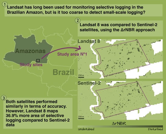
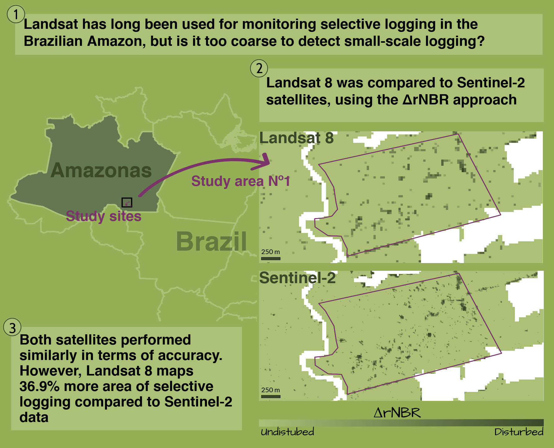
Comparing Sentinel-2 MSI and Landsat 8 OLI Imagery for Monitoring Selective Logging in the Brazilian Amazon

by
Thaís Almeida Lima
1,*,
René Beuchle
2,
Andreas Langner
2,
Rosana Cristina Grecchi
3,
Verena C. Griess
1 and
Frédéric Achard
2
1
Department of Forest Resources Management, Faculty of Forestry, University of British Columbia, Forest Sciences Centre, 2424 Main Mall, Vancouver, BC V6T 1Z4, Canada
2
European Commission, Joint Research Centre (JRC), 21027 Ispra, Italy
3
Independent Researcher, Via Piave 8A, 21020 Ranco, Italy
*
Author to whom correspondence should be addressed.
Remote Sens. 2019, 11(8), 961; https://doi.org/10.3390/rs11080961
Submission received: 12 March 2019 / Revised: 11 April 2019 / Accepted: 16 April 2019 / Published: 22 April 2019
(This article belongs to the Special Issue Assessing Changes in the Amazon and Cerrado Biomes by Remote Sensing)

Abstract

:
Imagery from medium resolution satellites, such as Landsat, have long been used to map forest disturbances in the tropics. However, the Landsat spatial resolution (30 m) has often been considered too coarse for reliably mapping small-scale selective logging. Imagery from the recently launched Sentinel-2 sensor, with a resampled 10 m spatial resolution, may improve the detection of forest disturbances. This study compared the performance of Landsat 8 and Sentinel-2 data for the detection of selective logging in an area located in the Brazilian Amazon. Logging impacts in seven areas, which had governmental authorization for harvesting timber, were mapped by calculating the difference of a self-referenced normalized burn ratio (ΔrNBR) index over corresponding time periods (2016–2017) for imagery of both satellite sensors. A robust reference dataset was built using both high- and very-high-resolution imagery. It was used to define optimum ΔrNBR thresholds for forest disturbance maps, via a bootstrapping procedure, and for estimating accuracies and areas. A further assessment of our approach was also performed in three unlogged areas. Additionally, field data regarding logging infrastructure were collected in the seven study sites where logging occurred. Both satellites showed the same performance in terms of accuracy, with area-adjusted overall accuracies of 96.7% and 95.7% for Sentinel-2 and Landsat 8, respectively. However, Landsat 8 mapped 36.9% more area of selective logging compared to Sentinel-2 data. Logging infrastructure was better detected from Sentinel-2 (43.2%) than Landsat 8 (35.5%) data, confirming its potential for mapping small-scale logging. We assessed the impacted area by selective logging with a regular 300 m × 300 m grid over the pixel-based results, leading to 1143 ha and 1197 ha of disturbed forest on Sentinel-2 and Landsat 8 data, respectively. No substantial differences in terms of accuracy were found by adding three unlogged areas to the original seven study sites.

Graphical Abstract

1. Introduction

Selective logging is a pervasive activity in tropical forests. In the Brazilian Amazon, it is a major source of forest degradation, possibly encompassing an area larger than that reported as deforested [1]. Despite the fact that carbon emissions caused by forest degradation in the tropics are to some extent compensated by forest regrowth [2], forests that have been selectively logged or burned store up to 40% less carbon than undisturbed forest stands [3]. Furthermore, previously logged forests, especially in the Brazilian Amazon, are at a higher risk of being converted into non-forest land use types [1].
The assessment of deforestation and forest degradation is a key component of international policies such as REDD+ (Reducing Emissions from Deforestation and Forest Degradation in Developing Countries). REDD+ policies require the use of reliable methods to measure carbon emissions from deforestation and forest degradation [4]. While Brazil has a consistent methodology for measuring deforestation [5], the approach used to estimate greenhouse gas emissions from forest degradation still needs improvement [6]. Forest degradation is defined by the Food and Agriculture Organization of the United Nations (FAO) as “the reduction of the capacity of a forest to provide goods and services” [7], a broad definition that needs to be contextualized for each country. Brazilian institutions still have to decide on a consistent and operational definition of “forest degradation”, while the development of a reliable monitoring methodology based on large-scale remote sensing analysis is equally indispensable. Brazil has had a prototype program to map forest degradation since 2007, called DEGRAD (Forest Degradation Mapping in the Brazilian Amazon) [8]. DEGRAD is based on a visual interpretation of moderate spatial resolution satellite imagery and has been used to map areas in process of deforestation, where the forest canopy cover has not yet been completely removed [8]. Therefore, research on automatic methods for mapping selective logging, a source of forest degradation, is imperative. As a result, the term “forest disturbance” is preferred, given that not all forest disturbance events necessarily result in forest degradation [9].
Despite the attempts to map anthropogenic forest disturbances in tropical forests using instruments such as the airborne light detection and ranging (LiDAR) [10,11,12], the use of freely available satellite imagery is currently the only feasible way of mapping changes over large areas of remote tropical forests. In the last two decades, several studies were carried out in the Brazilian Amazon with the objective of mapping or estimating areas of selective logging through optical remote sensing techniques [1,13,14,15,16,17,18,19,20,21,22,23,24,25,26,27,28,29,30,31,32,33,34,35,36,37,38]. These studies differ in terms of mapping units and protocols, type of remote sensing data analyzed, image processing techniques employed, geographic extent and location, total period of observation, and accuracy assessment. Some studies used very-high-resolution satellite imagery, such as IKONOS, to infer the total logged area and/or forest canopy disturbance size [17,19,24,39]. However, the vast majority of studies relied on moderate spatial resolution satellite imagery, notably from the Landsat program. Initially, these studies employed visual interpretation techniques to assess the total logged area [13,14]. At a later stage, a combination of (semi-)automated techniques, comprising a spectral mixture analysis (SMA) combined with a GIS analysis, were used to estimate the total logged area based on the location of log landings [15,18]. Automatic classification, based on fraction images derived from SMA, is currently the most common methodology used to detect and monitor selective logging in the Amazon [1,15,22,23,26,30,31,32,34,36].
Despite the remarkable improvements in mapping tropical forest disturbances in recent years, research gaps persist. For instance, the spatial resolution of Landsat imagery (30 m) can be too coarse to map small-scale forest disturbances in tropical forests, such as those resulting from selective logging [40]. The methodology proposed by Souza et al. [30], based on Landsat data, only detects forest disturbances that result in canopy openings of more than 25% within single Landsat pixels. However, disturbances caused by selective logging do not necessarily cause such large canopy openings. Consequently, there is a need to investigate the potential to map patterns of forest disturbances with finer spatial resolution. For many years, the lack of freely available imagery was the main barrier for doing so. However, the European Space Agency (ESA) recently launched the Sentinel-2A and Sentinel-2B satellites (in June 2015 and March 2017, respectively), making the data freely accessible. Sentinel-2A and 2B are “twin” satellites with the same optical sensor, providing multi-spectral imagery in 13 spectral bands at different spatial resolutions (10 to 60 m) with a revisiting time frequency of five days [41]. In the field of land use and land cover change, Sentinel-2 imagery has been used to map burned areas [42,43,44], to assess forest canopy cover properties [45], or to investigate the accuracy of Sentinel-2-based land use and land cover mapping [46]. However, studies addressing forest disturbances in tropical forests are still very few [47]. In this context, it is important to analyze the consequences of moving from the Landsat moderate spatial resolution to the finer spatial scale of Sentinel-2 data.
Previous studies have mapped forest disturbances using single-scene analysis of Landsat imagery per time period, which is usually one year [26,30,32,33,34]. However, in tropical evergreen forests, small-scale forest disturbance caused by selective logging activities can be recovered very fast (within a few months) by vegetation regrowth [40,47]. Therefore, the use of a single image for a given year can underestimate the amount of forest disturbances. For instance, in the Central Amazon, if a tree harvest is carried out in early dry season, with an image used in the analysis 4–6 months after the disturbance occurred, the mapped area is potentially underestimated due to the rapid vegetation regrowth. On the other hand, if the satellite image analyzed is acquired before a logging activity, the forest disturbance may not be detected at all in the subsequent year [37]. In addition, persistent cloud cover is a known problem in optical remote sensing analysis in tropical regions [48]. Since the opening of the Landsat archive, the analysis of image time series has become feasible, allowing the retrieval of spectral information without data gaps due to cloud cover [49].
Against this background, this study has two main objectives: (1) The mapping of forest disturbances caused by selective logging in seven sites under sustainable forest management (SFM) within the Brazilian State of Amazonas and (2) the comparison of the effectiveness of Landsat 8 data versus Sentinel-2 imagery for such purpose. To accomplish these objectives, we applied the “∆rNBR approach”—a modification of the normalized burn ratio (NBR) index—which has successfully been used to map forest disturbances in (semi-)evergreen forests in continental Southeast Asia [50]. Instead of working with single satellite scenes, this approach uses a time series analysis of all available satellite images and calculates the changes between two periods. Here, we applied the ∆rNBR methodology on imagery from both sensors during the dry seasons of years 2016 and 2017. We compared the resulting maps using accuracy assessment based on the visual interpretation of high-resolution images. To increase the robustness of our approach, three unlogged areas were also analyzed. Additionally, field data regarding logging infrastructure were collected and also used to assess the quality of the final maps.

2. Materials and Methods
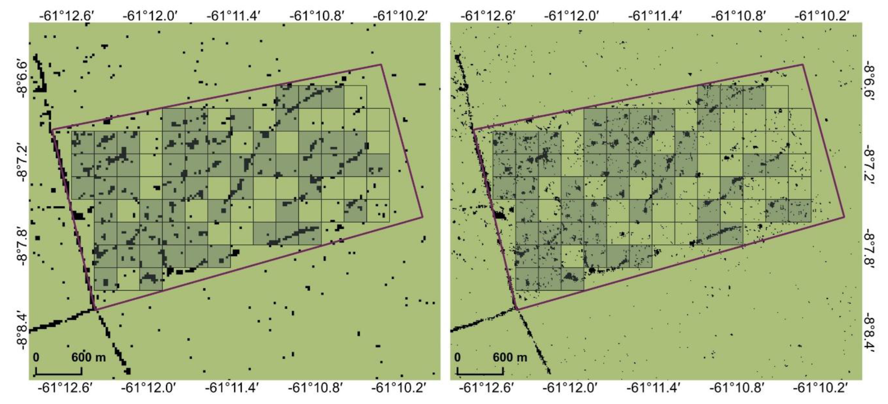
2.1. Study Area

The study area is located in the south of the Brazilian State of Amazonas. Amazonas is the largest state in Brazil (1.5 million km2) and holds the largest area of intact forests within the Brazilian Amazon [51]. This study was carried out in a focus area, bisected by the Transamazon Highway (BR 230), near the Village of Santo Antonio do Matupi (Figure 1). The area is one of the main timber production zones within the State of Amazonas [52]; the surrounding region is known as a deforestation hotspot [51].
The region has a tropical monsoon climate (Am) according to the Köppen climate classification system, with a recorded annual mean air temperature higher than 26 ºC and with annual rainfall ranging from 2800 to 3100 mm [53]. The short dry season (precipitation less than 60 mm per month) occurs between June and August [54]. The study area is covered by a mosaic of different vegetation types; with terra-firme forests (non-flooded) covering most of the region. These forests are classified as dense ombrophilous forest [55], with a tall, closed canopy.
To compare both sensors, we chose to focus our analysis on seven study sites where logging happened (areas 1 to 7) (Figure 1). These study sites are rectangular areas cropped from the satellite images and they overlap SFM sites. A further assessment of our approach was also carried out in three areas without logging activities (areas 8 to 10) (Figure 1). These areas were licensed as an SFM; however, harvest activities were not recorded for the time period where the mapping was performed. Herein, the term “sustainable forest management” follows the Brazilian legislation definition [56] and is used to define an area with governmental authorization for harvesting timber. In the State of Amazonas, by law, logging intensity is limited to 25 m3/ha, within areas suitable for timber extraction within each SFM area [57]. However, in general, the logging intensity is much lower than 25m3/ha (see Supplementary Materials, Table S1). All SFM areas comprise privately owned forests licensed in the years 2016 and 2017. In Brazil, the states have the responsibility of controlling the licensing process and issuing logging permits. In Amazonas, the Institute of Environmental Protection of Amazonas State (IPAAM) is responsible for issuing these permits. We chose our study sites from the IPAAM’s database, which contains all SFM areas licensed in the region of Santo Antônio do Matupi in the years 2016 and 2017. We selected these areas based on their ease of access and geographic distribution. The fact that each study site was located in an authorized logging area was crucial for security during field work.

2.2. Canopy Disturbance Mapping

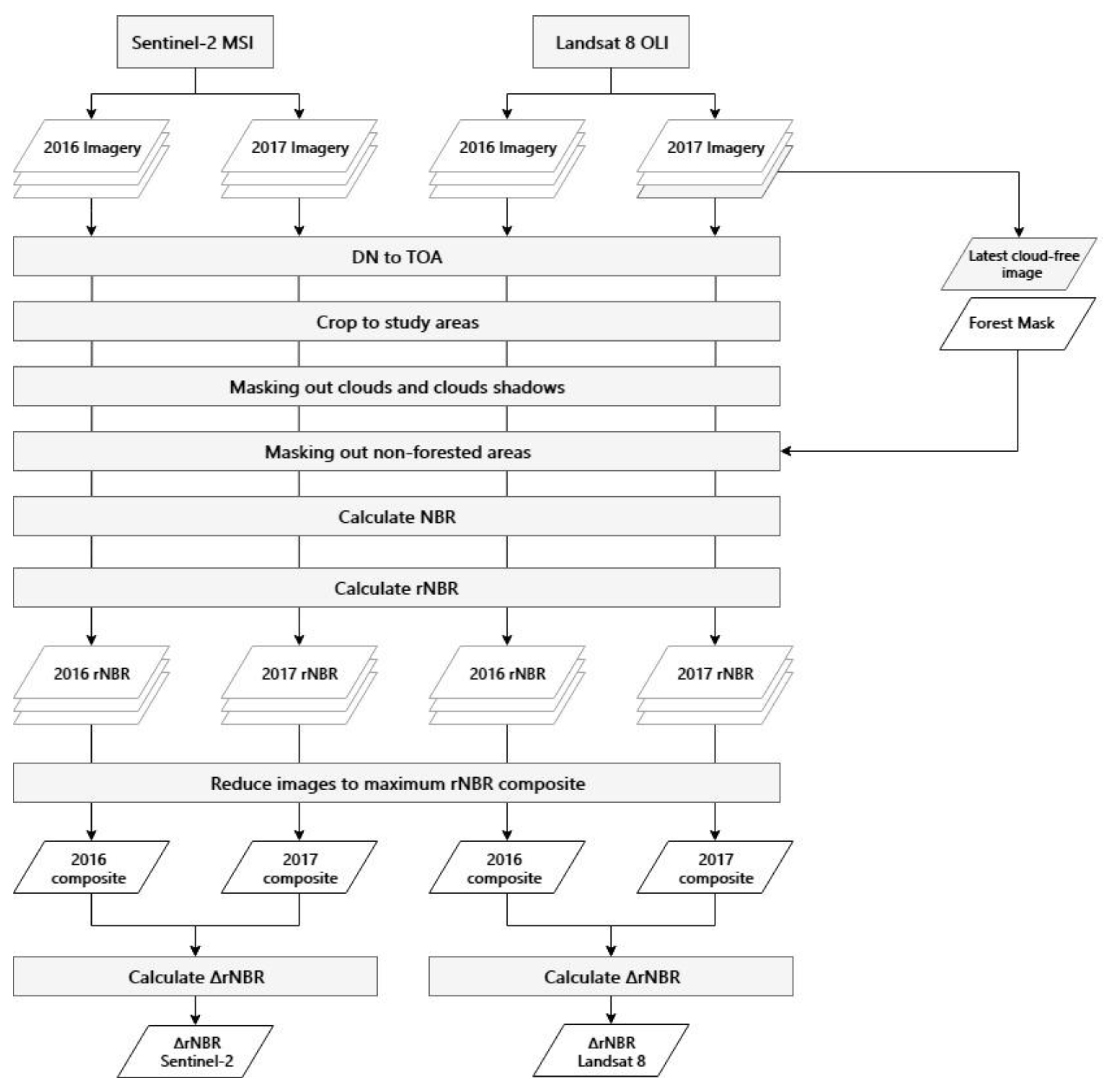
2.2.1. Satellite Imagery and Pre-Processing

Landsat 8 images (OLI/TIRS C1 Level-1) were obtained from the United States Geological Survey (USGS) Global Visualization Viewer (GloVis, https://glovis.usgs.gov). Sentinel-2 images (MSI Level-1C) were obtained from the European Space Agency (ESA) Copernicus portal (https://scihub.copernicus.eu). We analyzed all images (with less than 10% cloud cover) available for a 4-month time period from 1 June to 30 September, for 2016 and 2017. Choosing this timeframe allowed us to detect the temporal change in the spectral signal as close as possible to the canopy disturbance events. This is the case because logging activities in this region occur in the dry season and as explained before, this type of canopy cover disturbance recovers really fast. Therefore, by adopting this timeframe, the chance of getting a “logging event” can increase. A total of 17 images (eight from Landsat 8 and nine from Sentinel-2) were suitable and used in the consequent analyses (Table 1). A Sentinel-2A image from August 2015 was used to ratify that the target areas had not been disturbed in the previous year.
For Landsat data, raw digital numbers (DN) were converted to top-of-atmosphere (TOA) reflectance values following Reference [58]. For Sentinel-2, we kept the original Level-1C TOA reflectance values. The corresponding spectral bands available for both sensors were taken into account in this process: Blue, green, red, near infrared (NIR), short-wave infrared 1 (SWIR-1), and short-wave infrared 2 (SWIR-2). The SWIR-2 band in Sentinel-2 imagery comes at a 20 m resolution, therefore it was resampled to 10 m resolution using the nearest neighbor resampling method. For Sentinel-2 imagery, considering land use and land cover maps, downscaling has been shown to have superior performance compared to upscaling, even when based on the most straightforward technique, the nearest neighbor resampling [59]. For this reason and also because we aimed at small-scale disturbances, downscaling was preferred over upscaling. Subsequently, all images were cropped to match the study sites. These steps were completed using the image processing (IMPACT) toolbox from the European Commission [58].
Even though images with low cloud cover were selected, clouds could not be fully avoided. Thus, we applied a semi-automatic object-oriented approach to mask out the clouds and cloud shadows. First, a multiresolution segmentation [60], using the three visible bands of the electromagnetic spectrum, was performed in eCognition® software. Afterwards, given the small size of the study sites and the limited cloud cover, it was possible to carry out a visual interpretation to remove image objects labelled as clouds and cloud shadows. Despite being labor intensive, a careful visual interpretation was preferred over a fully automatic approach for our limited-extent study areas, to avoid cloud omission errors which may have led to false disturbance detections.

2.2.2. Building a Forest/Non-Forest Mask

To eliminate non-forested areas from our dataset, we applied an object-based image analysis on the latest Landsat 8 image from the second year (2017), following a methodology proposed by Grecchi et al. [34]. Non-forested areas included water bodies, natural vegetation not classified as forests (e.g., savannas), and deforested areas. For this study, deforestation follows the definition of FAO [7] meaning “the conversion of forest to other land use”. This step was required to avoid wrongly classifying some areas of selective logging as deforestation (e.g., log landings). Therefore, logging infrastructure, such as log landings and logging roads, were kept inside the forest mask and were mapped as a part of the forest disturbance process. To build this forest mask, a segmentation process, aiming at a minimum mapping unit (MMU) of 3 hectares (ha), was performed in eCognition®. Objects smaller than 3 ha were then merged to comply with the defined requirements for MMU. A decision-tree classification approach was applied to categorize image objects into three main classes: Forest, non-forest, and water. Previously, we performed an unconstrained linear spectral mixture analysis [61] to get three fraction images: Soil, vegetation, and water/shadow. This step was completed using the IMPACT toolbox, where unconstrained values were rescaled to values between 0–255 [58]. All image objects with a soil fraction mean ≥108 were classified as non-forest and all objects with a water fraction mean ≥185 and a mean value for the NIR band <70 were classified as water. All remaining objects were classified as forest.
Finally, the classification was exported as a raster file, with a binary classification: Forest with value 1 and non-forest with value 0. As this binary forest mask was built using a Landsat image, a nearest neighbor resampling technique was carried out to convert the forest mask to the spatial resolution and the geolocation of the Sentinel-2 images. The quality of the forest mask was assessed in the seven study sites where logging occurred (areas 1 to 7), based on the visual interpretation of the latest Landsat image from the year 2017, which was carried out by an external expert. A stratified random sampling scheme was applied for the two strata (forest and non-forest areas) with 150 sampling points for each one, distributed randomly over the seven study sites. The area-adjusted overall accuracy [62] was 98.6%, with adjusted producer’s accuracy of 99% for the forest class and 95.7% for the non-forest class. The area-adjusted user’s accuracy was 99.3% for the forest class and 94% for the non-forest class.

2.2.3. Applying the ∆rNBR Approach

To detect canopy cover disturbance, a ratio-based vegetation index called normalized burn ratio (NBR) was used. The NBR index is based on the normalized difference of the NIR and the SWIR-2 bands (Equation (1)). NBR is particularly sensitive to changes in live green vegetation [63]. Like the normalized difference vegetation Index (NDVI), the NBR output is composed by floating point values ranging from −1 to 1, where larger positive values are linked to closed forest canopy cover and smaller positive or even negative values indicate openings in the canopy cover [50]. The NBR was calculated for all images used in this study.
N B R = N I R S W I R 2 N I R + S W I R 2
The NBR index has been traditionally used to map burn severity [63]. However, recently, it also has been used to assess forest disturbances, such as those caused by selective logging [64]. To detect changes in a given area, the NBR is assessed before (period 1) and after (period 2) the disturbance event. The difference between the values calculated for period 1 and period 2 is called ΔNBR.
When used to assess small-scale forest disturbances, NBR values can be different for two dates, even in the absence of forest cover change. This NBR difference can be due to unequal atmospheric conditions or illumination geometries [47]. To avoid assigning such change as a signal of forest disturbance, Reference [50] further developed the initial NBR methodology by introducing a self-referencing step. This approach is based on a moving window concept, which aims to account for the similarity (or dissimilarity) a given pixel has in comparison with its neighborhood [65]. Therefore, this self-referencing step shifts the NBR values to zero by subtracting the original NBR values at each pixel location from the median of the NBR values within a circular window centered at the pixel (Equation (2)). By following this method, intact forest canopies result in values close to 0, while openings in the canopy cover that expose bare soil or non-photosynthetic vegetation show positive values. Following Reference [50], we chose a 210 m radius as the size of the moving window.
r N B R = N B R n   m e d i a n N B R
As the impacts of logging infrastructures on spectral signatures are ephemeral, we calculated the rNBR for all available images from the beginning to the end of the dry season (June to September) of a given year and then aggregated the maximum rNBR values into a single annual composite. The ΔrNBR image was then produced from the two annual image composites of max rNBR of years 2016 and 2017 (Equation (3)). All these steps (Figure 2) were developed with “R” software [66], using the raster package [67]. Image composites were created using a Python script provided by Reference [68].
Δ r N B R = r N B R P e r i o d   2 r N B R P e r i o d   1

2.2.4. Detecting Forest Disturbances from Optimized Thresholds

A common approach used to assess the spectral signals of forest disturbances from remote sensing analyses is the empirical definition of thresholds [69]. Accordingly, an empirical threshold value is defined to build a binary map, encompassing areas considered “disturbed”, “degraded”, or “logged”, depending on the adopted method and terminology [30,33,34]. For both Landsat 8 and Sentinel-2 imagery, we decided to produce binary maps for different ΔrNBR thresholds, ranging from 0.001 to 0.200 (200 values in total), and to compare the resulting sets of binary maps with a reference dataset, in order to define an optimum threshold value.
The seven study sites where selective logging occurred (areas 1 to 7, Figure 1) were used to define the threshold values for both sensors. The reference dataset used for choosing the best threshold values was built using a combination of high- and very-high-resolution imagery (spatial resolution <10 m). PlaneScope® images, with a 3 m spatial resolution, from the end of the dry season of both years (2016 and 2017), covering five of the seven SFM areas, were used to assess if the areas were logged or not (Supplementary Materials, Table S2). For two areas, a GeoEye-1 image (0.43 m spatial resolution), available in the Google Maps API®, was used for the interpretation of logging activities for the year 2017, while PlaneScope® imagery were used to assess the pre-logging status of the forests in 2016. To label the reference dataset in two distinct classes, disturbed or undisturbed, a visual interpretation was carried out for 600 sample points. To be included as a change event, the areas needed to be clearly identified in the images as logging areas or logging infrastructure. Areas with doubtful interpretation were not included in the reference dataset.
The number of sampling points was chosen based on the assumption that the areas would not have experienced more than 15% of land cover change. This assumption is reasonable because the change event is considered as a rare event in the landscape [70], and even rarer if we take into account that the study areas are under sustainable forest management. Therefore, assuming area proportions for the stable class forest (i.e., undisturbed class) as 0.85 and 0.15 for the change class (disturbed), a target user’s accuracy of 0.95 and 0.80 for the undisturbed and disturbed class, respectively, and a standard error for the overall accuracy of 0.01, leads to the number of sample points of approximately 600, according to the equation for stratified random sampling presented by Reference [62]. Considering the stratified random sampling scheme, different distributions of the total number of samples amongst different strata will favor different estimation objectives [62]. In our case, we wanted to be sure that the areas of logging were correctly included in the map (i.e., minimizing errors of omission), therefore 100 sample points were chosen for the class of disturbance and 500 sample points for the forest (undisturbed) class, with 100 of them allocated in the three study sites known to be unlogged.
To determine optimum threshold values, we followed a bootstrapping procedure [71]. The use of resampling methods, such as bootstrapping, has been reported as a more robust approach than a single split of the data into training and test sets [72]. From a total of 600 sample points, a random sample of 350 points was extracted and the estimated overall accuracy [62] was calculated from this sub-sample for each of the 200 binary maps. This procedure was iterated 1000 times while for each iteration we recorded the ΔrNBR value that maximized the overall accuracy. Subsequently, we calculated the average threshold values for each satellite sensor, herein called “optimized thresholds”. These optimized thresholds were then used to build the final canopy disturbance maps used for comparisons between Landsat 8 and Sentinel-2 imagery (Figure 3).

2.2.5. Assessing Forest Area Affected by Selective Logging Using a Grid Approach

In order to assess the forest area impacted by selective logging, we applied a regular grid of 300 m × 300 m spatial resolution on the pixel-based results from both sensors, leading to 252 full grid cells over the forest of the seven SFM areas. The size of the grid cells is similar to a radius of 180 m from the mapped disturbance areas, as proposed by References [15] and [21], to assess the forest area directly or indirectly affected by selective logging. The grid area typically contains features such as smaller sized logging infrastructure (small felling gaps, narrow logging roads, skid trails) and residual damaged vegetation due to the logging operations [73], which are not detectable by remote sensing imagery. In addition, due to the use of permanent assessment units, a grid cell approach has the advantage of enabling a long-term assessment of the forest disturbances related to selective logging, which is highly dynamic in space and time. A grid approach with the same grid cell dimensions has been used to monitor selective logging with Landsat imagery over 15 years in Mato Grosso State by Reference [34].
Grid cells that contained less than 5% of pixel-based mapped selective logging area were not taken into account in order to avoid results compromised by random effects.

2.3. Accuracy Assessment and Field Data Collection

For the accuracy assessment of the disturbance maps, the entire reference dataset (i.e., all 600 sampling points mentioned above) were used for building the error matrix, and for estimating accuracies and areas for both sensors [62].
Our approach was further applied to three unlogged forest management units (areas 8 to 10, see Figure 1) and an additional accuracy assessment was done after the inclusion of these new areas. The three unlogged areas were mapped using the same approach adopted for the forest management units where logging occurred (areas 1 to 7, see Figure 1). The binary maps, derived from the best threshold values, were compared with a new reference dataset built to also include sampling points in these three unlogged areas. Accordingly, 200 sampling points were randomly assigned for the forest (undisturbed) class. Therefore, the new reference dataset had 800 points, 700 for undisturbed forest and 100 for the disturbed forest.
With support of the State of Amazonas Government through IPAAM, we visited SFM areas near the Village of Santo Antônio do Matupi. The field data collection was carried out during IPAAM’s law enforcement inspections in the region in the first and second weeks of October 2017. In the seven SFM areas, we collected GPS locations and information regarding the type of logging infrastructure: Log landings, felling gaps (canopy gaps created by the process of felling trees), logging roads, and skid trails (Figure 3).
Although we initially intended to use a random sampling scheme, the field data collection was changed towards the selection of points close to logging roads. We collected field data for 155 sample locations, distributed over the 7 SFM areas. Consequently, the collected field data were not used for accuracy assessment, but for a quantitative comparison with the resulting disturbance maps to infer the degree of “detectability” of disturbances from our mapping approach. The field points could not have been used for accuracy assessment due to the limited number of sampling points; also, because some of the impacts provoked by logging activities do not result in canopy cover removal, as in the case of some portions of logging roads and skid trails (Figure 3). In spite of this, the field points helped to distinguish the logging infrastructure when the reference dataset was built. The percentage of GPS points corresponding to logging infrastructure that overlap the final (optimized) disturbance maps was used as detectability performance criteria.

3. Results

3.1. Optimized Thresholds

The bootstrapping approach used to retrieve the optimized thresholds (Figure 4) shows that the overall accuracy had low values for the lowest threshold values (due to a high error of commission) and then increased strongly until peak threshold values at around 0.03 and 0.06 for Landsat 8 and Sentinel-2, respectively. Subsequently, the overall accuracy dropped with increasing threshold values, due to a high error of omission. Our simulations of disturbance maps resulted in optimized threshold averages for ΔrNBR at 0.035 (±0.005) and 0.065 (±0.009) for Landsat 8 and Sentinel-2 images, respectively.

3.2. Sentinel-2 versus Landsat 8

3.2.1. Accuracy of Disturbance Detection

The overall accuracy of the two mapped classes (disturbed forest and undisturbed forest), taking into account the original, uncorrected error matrices, was 94.8% for Landsat 8 and 94.3% for Sentinel-2. When adjusted to account for area proportion, these values increased. The area-adjusted overall accuracies for Landsat 8 and Sentinel-2 were 95.7% and 96.7%, respectively (Table 2). The omission error was higher for the disturbed class for both satellites. Here, the area-adjusted producer’s accuracy for the disturbed class was 59.3% for Landsat 8 and 63.3% for Sentinel-2. On the other hand, the area-adjusted producer’s accuracy for the undisturbed class (stable class, with no change) was 99.2% and 98.9% for Landsat 8 and Sentinel-2, respectively (Table 2).
No substantial differences in terms of accuracy were found by adding three unlogged areas to the original seven study sites. Taking into account the 10 areas, the area-adjusted overall accuracies for Landsat 8 and Sentinel-2 increased marginally, with values of 96.7% and 97.5%, respectively. This can be explained by the high accuracies recorded for the undisturbed class. For this class, the area-adjusted user’s accuracy was 97.4% and 98.3% for Landsat 8 and for Sentinel-2, respectively. The area-adjusted producer’s accuracy was 99.1% for both sensors. However, for the disturbed class, the area-adjusted producer’s accuracy showed a slightly decrease for the Sentinel-2 map (62.1%) while for Landsat 8 it was recorded the same accuracy of before (59.3%). The area-adjusted user’s accuracy for the disturbance class also decreased, with new values of 80.4% and 77.2% for Landsat 8 and Sentinel-2, respectively.

3.2.2. Forest Area Affected by Selective Logging: Pixel-Based Approach

Considering the disturbance maps derived from the proposed approach and calculating the area covered by pixels with values greater than the optimized thresholds, Landsat 8 imagery led to the detection of a larger logging-affected area than Sentinel-2 imagery (Table 3). The adjusted area for the disturbance class was 282.7 ± 52.5 ha for Landsat 8 and 206.5 ± 44.1 ha for Sentinel-2. The map based on Landsat 8 led to an area affected by selective logging 17.8% higher than the map based on Sentinel-2 data, considering the simple pixel counting. However, when adjusted areas are taken into account this value was 36.9%. There was an uncertainty associated with the choice of the best threshold value, particularly for Sentinel-2 (ΔrNBR ≥ 0.065 ± 0.009). If we were to consider the lower end of this uncertainty interval (i.e., ΔrNBR ≥ 0.056) and the areas computed by simple pixel counting (Table 3), the logged areas mapped by Sentinel-2 would be substantially higher (163.4 ha for ΔrNBR ≥ 0.065 and 201.3 ha for ΔrNBR ≥ 0.056). Even if the differences in the overall accuracy for the lower end (96.6% for ΔrNBR ≥ 0.056) seem to be minimal, the commission error increased, reaching a value of 26.6%. By choosing to use the optimized threshold, i.e., the mean of all values that maximized the overall accuracy in 1000 simulations (ΔrNBR ≥ 0.065), we were able to avoid this problem.
The percentages of logged area in relation to the total SFM areas (Table 4) varied from 2.43% to 14.28% for Landsat 8 and from 1.91% to 11.60% for Sentinel-2. In total, over the seven SFM areas, the percentages were 5.73% and 4.87% for Landsat 8 and Sentinel-2, respectively. If we analyze the sum of pixels classified as disturbed within the three unlogged sites the resulting areas are negligible for Sentinel-2, with 0.6% of the total area accounting for disturbed pixels, for all sites. However, for Landsat 8, these disturbed pixels result in 1.2%–2.6% of the total areas.

3.2.3. Forest Area Affected by Selective Logging: Grid-Based Approach

From the 252 full grid cells of 300 m × 300 m over forest in the seven SFM areas, 127 grid cells (1143 ha, 50.4%) and 133 grid cells (1197 ha, 52.8%) contained more than 5% of pixels of mapped selective logging in Sentinel-2 and Landsat 8 data, respectively (Figure 5). The difference between the two sensors thus resulted in a 4.7% larger area with Landsat imagery. The grid cells appearing as disturbed in both datasets amounted to 116, accounting for 91.3% and 87.2% in Sentinel-2 and Landsat 8 data, respectively. In addition, we applied a sensitivity analysis on the position of the grid cells by calculating the statistics over ten different grids; nine of them shifted by 75 m steps in E-W, N-S and both directions from the original grid. In all cases, Landsat 8-based results showed a larger area of impacted forest by selective logging, ranging from 1.6% to 12.5%, with an average of 6.8%, compared to results based on Sentinel-2 imagery.

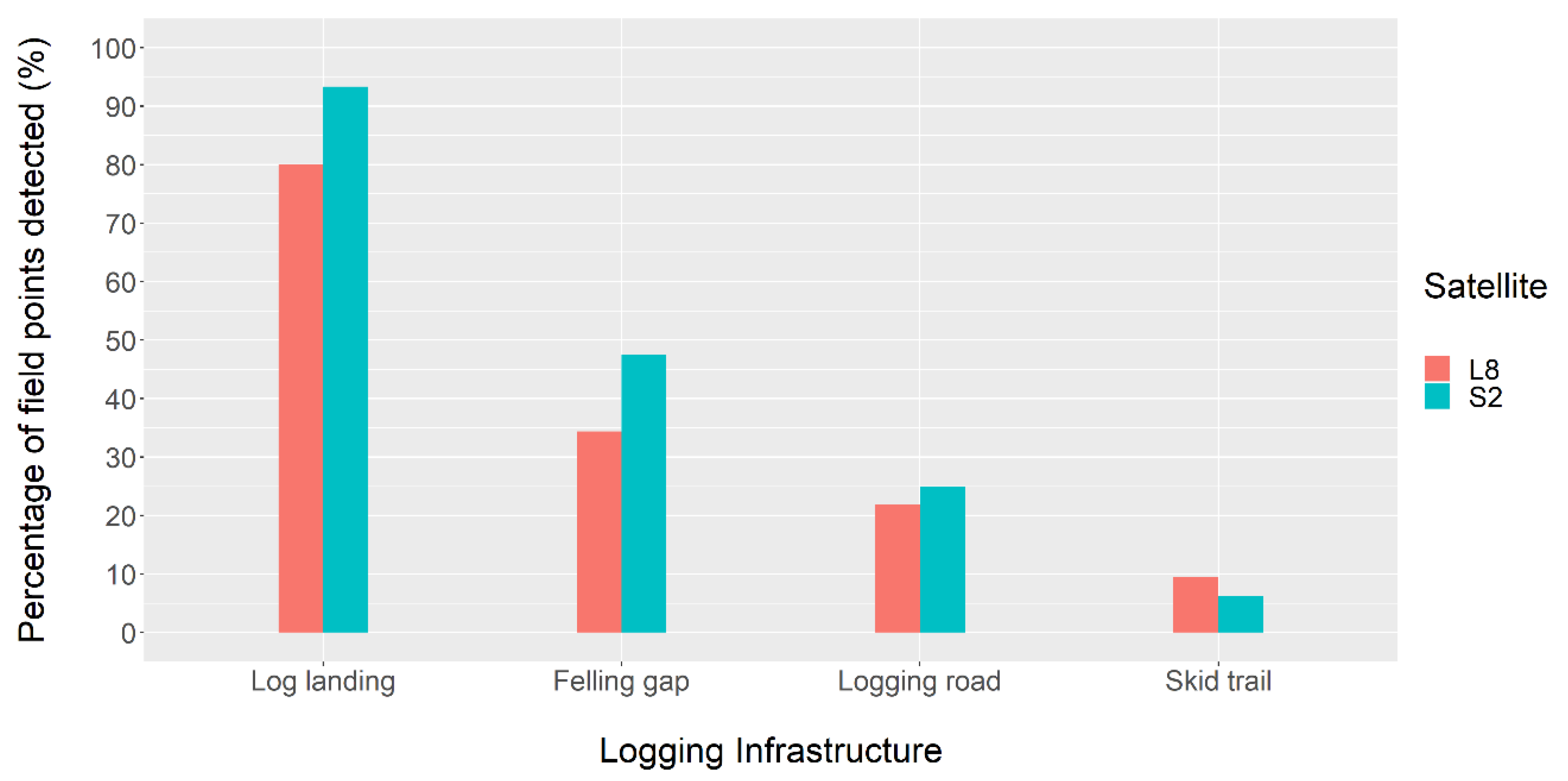
3.3. Detectability of Logging Infrastructure: Results from Field Data Collection

During field data collection, the geolocation of 155 sampling points was collected, and distributed throughout the seven study areas. Data were collected for the geographic location and major types of logging infrastructure present. Logging infrastructure catalogued includes log landings (30), felling gaps (61), logging roads (32), and skid trails (32).
When comparing the field information to our disturbance maps, it appeared that Sentinel-2 imagery had a better capability for detecting logging infrastructure than Landsat 8 imagery (Figure 6). For log landings, the percentage of correct detection was 93.3% and 80% for Sentinel-2 and Landsat 8 imagery, respectively. However, for other types of logging infrastructure we did not observe the same pattern. Felling gaps, with the second highest percentage of correct detection, reached 47.5% and 34.4% for Sentinel-2 and Landsat 8 imagery, respectively. Logging roads (Landsat 8 = 21.9% and Sentinel-2 = 25%) and skid trails (Landsat 8 = 9.4% and Sentinel-2 = 6.3%) showed very low percentage values of detectability.

4. Discussion

4.1. Detection of Logging Impacts: Comparison with Other Studies in the Amazon

Based on the ΔrNBR approach proposed by Reference [50], selective logging activities were mapped in the seven SFM areas near the town of Santo Antônio do Matupi, State of Amazonas, Brazil. The area-adjusted overall accuracies in the present study were satisfactorily high, with 95.7% for Landsat 8 and 96.7% for Sentinel-2, respectively. Similar values were obtained by Reference [34] for a forest disturbance mapping performed in the Brazilian Amazon, using SMA analysis on Landsat imagery, as well as in other studies [30,31].
Instead of choosing arbitrary thresholds, our methodology allows for the selection of an optimized threshold for each sensor, Landsat 8 and Sentinel-2, through the use of a reference dataset. The optimized thresholds were defined using a bootstrapping approach with numerous simulations of accuracy assessments, with the goal of minimizing commission and omission errors, leading to the highest overall accuracy. For both satellites, the user’s and producer’s accuracies for the disturbed forest class was much lower than for the undisturbed class (Table 2). Omission errors play a major role in lowering the overall accuracy at the best possible threshold. With decreasing threshold values, overall accuracies also decreased considerably (Figure 4), indicating a strong increase of commission errors due to noise effects over non-disturbed areas. Therefore, it is possible that the key to more accurately identify disturbed areas does not lie in the lack of “detectability” through the ΔrNBR index, but rather in the capacity to separate real forest disturbances from noise. Notwithstanding, the range of all accuracies found here are well within the range of previous works, or exceed them [30,31,34,38,50].

4.2. Sentinel-2 versus Landsat 8

4.2.1. Accuracy Assessment

Several studies have been carried out on sensor comparison and synergistic use of Landsat 8 and Sentinel-2 [43,45,46,74,75,76]. However, more information is needed regarding the differing capabilities of the two sensors for land cover mapping and the consequences of these differences in the context of forest cover monitoring and forest cover change assessment. Our results of mapping forest disturbances with the ΔrNBR approach reveal that, although Sentinel-2 shows a better performance, the overall accuracy (96.7%) is just marginally higher than the one reported for Landsat 8 (95.7%). Similar values were reported in other studies on land cover changes when comparing Landsat 8- and Sentinel-2-based results. For instance, Reference [46], mapping land use and land cover in Burkina Faso, found that the usage of Sentinel-2 data can improve image classification accuracy by 4%. In another study, Sentinel-2 was also shown to better map burn scars and fire severity in Greece from a ΔNBR approach with a 2.7% higher overall accuracy compared to Landsat-based results [42]. A study in Finland [45] compared the retrieval of biophysical variables for forests, concluding that Sentinel-2 performed better when the red-edge band was taken into account, however, the improvements in accuracy were marginal.
Sentinel-2 has very similar spectral bands compared to Landsat 8; therefore, a better detectability of selective logging was expected due to the finer spatial resolution of Sentinel-2. However, Landsat 8-based results have similar overall accuracy. This could indicate that despite its coarser spatial resolution, Landsat 8 has a good potential to identify logging features. These results agree with recent studies carried out in a region near the study area, in the State of Rondônia, Brazil [36,37]. However, the area mapped as logged with Landsat imagery is considerably larger in comparison with Sentinel-2-based results.

4.2.2. Forest Area Affected by Selective Logging

Landsat 8 data increased the estimated area of selective logging by 36.9%, compared to Sentinel-2 (Table 3). Logging infrastructure, such as log landings and logging roads, are generally smaller than the Landsat spatial resolution [38]. In consequence, the possible area overestimation can be attributed to the high response values of mixed pixels in Landsat 8, that show up as a set of “pure” pixels in Sentinel-2, for the same corresponding area. Even though Sentinel-2-based results have a higher commission error for the disturbed class (20%) compared to Landsat 8 results (12.9%), this was not reflected in an increase of the mapped area. From Figure 3 it is clearly visible that Landsat 8 correctly detects most of the logging infrastructure that results directly in canopy cover reduction. However, with its 30 m spatial resolution, it will also include “non-directly affected” logging areas in the same mapping unit (i.e., the pixel), leading to a larger mapped area. The three areas without logging activities showed a minimal number of pixels classified as disturbed (0.6% for Sentinel-2). For Landsat 8, these disturbed areas represented from 1.2% to 2.6% of the total areas, reflecting its coarse spatial resolution. Given the high response values of the ΔrNBR for these pixels and the scattered spatial distribution of them, it is possible that they represent natural disturbance events, such as natural tree falls. A further spatial pattern analysis could be useful to “filter” these isolated pixels from the original mapping, if one is interested in reporting disturbed areas in a regional scale, for example.
Deleterious effects of selective logging in tropical forests are not restricted to canopy cover reduction, but have cascading effects on rates of forest growth, hydrological processes, and carbon cycling [77], and can have negative impacts on wildlife [78]. Artificial gaps created by selective logging activities, despite being designed to emulate natural systems (gap phase dynamics), lead to a larger disturbance area than is expected to occur under natural gap phase dynamics [79]. Previous remote sensing studies deduced the area affected by selective logging, using buffers around key logging infrastructure [15,27], as a way to estimate logging impacts throughout surrounding forests. However, considering the areas under investigation, it is virtually impossible to affirm that the non-directly affected areas of forests mapped from Landsat 8 imagery are necessarily disturbed or even degraded, without consistent field data and a reliable methodology for concluding so.
Logging authorizations within the State of Amazonas are valid for 24 months. Therefore, logging activities can be carried out over the course of three consecutive years. Our research focused on areas with logging authorizations starting in 2016. In consequence, it was probable that logging activities would be carried out within the following 12 months. During the field campaign (carried out in 2017), it was observed that the SFM activities were almost completely finished, however, a small percentage of the authorized logging could potentially have occurred also within 2018. There is no clear relationship between logging intensity and the percentage of the SFM area mapped as logged (Table 4). This can be explained by two main reasons. First of all, the logging intensity is quite similar amongst areas. Second, logging intensity is just a ratio between the volume authorized for logging and the total area of the SFM. The percentage of disturbed areas will also be dependent on the spatial distribution of logging activities and on the impacts of selective logging on the remaining vegetation during the harvest process. For instance, if two areas have the same logging intensity, but one of them did not follow the guidelines for minimizing harvest impacts, this area will have a high percentage of disturbed areas. In spite of this, the percentages of logged forest area, considering all SFM areas analyzed (Landsat 8 = 5.73%; Sentinel-2 = 4.87%), were similar to those reported from other studies carried out in areas under reduced impact logging (RIL) techniques and/or subjected to legal harvest constraints (like SFM). The logging intensity in the study sites is lower in comparison with the maximum volume authorized by law [56,57] and more related to other studies carried out following RIL and/or low impact logging [12,16]. The authors of Reference [16], working in the Eastern Brazilian Amazon, found that the ground disturbance in areas subjected to RIL (logging intensity 23 m3/ha) was circa 4.6%–4.8%, in relation to the total area authorized for selective logging. Authors of a different study [33], also focusing on the Eastern Brazilian Amazon, reported an average of 5% disturbance in RIL logging plots. While mapping selective logging with aerial LiDAR and field data in the State of Acre, in a public forest following very low harvest intensities (up to 13.3 m3/ha), Reference [12] recorded areas of logging ranging from 7% to 8.6%. However, in areas undergoing illegal/conventional logging, these percentages could be higher [16,33].
All RIL practices are not mandatory by law and SFM plans only need to comply with constraints present in the current Brazilian environmental legislation. These may include RIL practices or they may not [80]. One of the few constraints that allows monitoring with remote sensing techniques is related to the authorized area of forest openings for the construction of log landings and logging roads, currently limited to 2.5% of the total area of the management unit [57]. However, the legislation does not establish any limits for the openings of felling gaps. We were not able to clearly separate the damage caused by log landings and felling gaps in our study sites. In this context, it would be reasonable, as a suggestion for decision makers, to adapt the law to set a limit for the “total area under disturbance” which would include also the disturbances caused by felling gaps, rather than to specify maximum percentages by the type of logging infrastructure.

4.2.3. Grid Cell Approach Measuring Affected Forest Area by Selective Logging

The grid-based comparison of forest area affected by selective logging in Sentinel-2 and Landsat 8 data does not reflect the large difference of 36.9% between the sensors in the pixel-based forest disturbance mapping approach. The respective value for the grid-based area comparison (6.8% overestimation with Landsat 8) shows that most of the pixel-based overestimation by Landsat data was compensated in the grid by the spatial proximity of the Landsat 8 and Sentinel-2 disturbance pixels. In consequence, as for the pixel-based approach, the overestimation of the Landsat-based analysis is mostly linked to the coarser resolution.

4.2.4. Detectability of Logging Infrastructure

The logging infrastructure detectability was calculated using data collected from 155 field plots across the seven SFM areas. Sentinel-2 has a better capability for detecting logging features (43.2%) compared to Landsat 8 (35.5%), which can most likely be attributed to its finer spatial resolution. The detectability over all types of logging features was similar to values reported by Reference [1].
In a study performed in Guyana that mapped logging activities with Sentinel-2 data, it was noted that skid trails could not be identified using Sentinel-2 imagery [81]. This highlights the fact that skid trail damage is almost impossible to detect with optical remote sensing data available today because of its “below canopy” location (Figure 3). The logging roads in our study areas are secondary roads, built to be temporary and ranging from 4 m to 6 m in width. This could explain the lack of “detectability” for this kind of infrastructure. Nonetheless, the detectability of logging features confirms a better performance by Sentinel-2 (Figure 6), even if the difference from Landsat 8-based values is small. However, given the higher spatial resolution of Sentinel-2, these differences between the sensors are smaller than expected.

5. Conclusions

In this study, we compared the performance of the Sentinel-2 MSI and Landsat 8 OLI sensors for detecting forest canopy disturbances caused by selective logging in a focus area in the State of Amazonas, Brazil. We combined a novel approach for detecting forest disturbances, the ΔrNBR index [50], with a robust methodology to select optimized ΔrNBR thresholds for mapping forest disturbances in seven sustainable forest management areas harvested during years 2016 and 2017. The area-adjusted overall accuracy for both sensors were similar, with a slightly higher accuracy recorded for Sentinel-2. No large differences in terms of accuracy were found by adding three unlogged areas to the original seven study sites. Taking into account the area mapped as disturbed, we found that Landsat 8 overestimates the detection of logging by approximately 36.9%, when compared to Sentinel-2 data. Using field data collected in the seven sustainable forest management areas, we reported that Sentinel-2 imagery allows for the better detection of log landings and felling gaps than Landsat 8 imagery. However, other logging features had a small detection percentage for both satellites.
We expected to find more substantial differences between the maps derived from Landsat 8 versus Sentinel-2 data, given the nature of the forest disturbances investigated. However, our results show similarities between the two sensors, both in terms of accuracy and logging infrastructure detectability using field data. This provides evidence of the potential for interoperability of the two sensors’ data in the context of forest canopy cover change. Moreover, it was shown that Landsat 8 maps larger areas containing forest disturbances, compared to Sentinel-2, both in the pixel-based and grid-based approaches, due to the lower spatial resolution. However, the two approaches deliver very different figures of Landsat overestimation, with the grid-based overestimation being much smaller than the pixel-based approach. The higher spatial resolution of Sentinel-2 leads to a more precise pixel-based mapping of forest disturbance by selective logging, making it possible to map smaller disturbances and to map larger disturbances more precisely. For pixel-based forest disturbance maps, it becomes clear that results should be called “areas of occurrence of selective logging” rather than “areas of selective logging” because considerable parts within Landsat pixels do not cover logging infrastructure. This is reflected by the large difference of pixel-based mapping results with Landsat and Sentinel-2 sensors. Future research could focus on more precise estimates of Landsat products for mapping areas directly affected by logging, using, e.g., a change area correction factor, as suggested for MODIS products [82]. In addition to this, future comparisons of Landsat 8 and Sentinel-2 could analyze possible synergies with the additional bands present in Sentinel-2, such as the red edge bands and the narrow NIR band, which were not investigated in the present study.

Supplementary Materials

The following are available online at https://www.mdpi.com/2072-4292/11/8/961/s1, Table S1: Information about the sustainable forest management (SFM) plans implemented in the seven forest management units (FMU) analyzed in this study. These data were disclosed by the Brazilian Government, represented by the Institute of Environmental Protection of Amazonas State (IPAAM), under the Administrative Process Nº1946/2017; Table S2: Reference data set used in this study.

Author Contributions

Conceptualization, T.A.L. and R.B.; methodology, T.A.L. and R.B.; validation T.A.L. and R.B.; formal analysis, T.A.L.; investigation, T.A.L.; data curation, T.A.L.; writing—original draft preparation, T.A.L.; writing—review and editing, T.A.L., R.B., A.L., R.C.G, V.C.G., and F.A.; visualization, T.A.L.; project administration, T.A.L.; funding acquisition, T.A.L. and V.C.G.

Funding

This research was funded by: The International Tropical Timber Organization (ITTO) (Grant Nº017/16A); the Institute of Environmental Protection of Amazonas State (IPAAM) and by the Idea Wild Foundation; This article is part of T.A.L.’s PhD project, which is funded by the University of British Columbia (Vancouver, Canada).

Acknowledgments

We would like to thank: the Amazonas State Government and IPAAM for their logistic support during the field campaign; the analysts from IPAAM Aline dos Santos Britto and Raimundo Saturnino de Andrade for their help during the field data collection; the foresters Fabio Azevedo, Thuany Bitencort and Marilia Caporazzi for their logistic support in the Village of Santo Antônio do Matupi. We are also very thankful to Ghislain Vieilledent (CIRAD) for the useful advices about resampling techniques and Anelena Lima de Carvalho (UFAC) for reviewing the paper. We express our gratitude to the Planet company, who provided free access to PlanetScope imagery through the Planet’s Education and Research Program. This research was carried out during the time T.A.L. spent as a visiting researcher at the Joint Research Centre (JRC), under the Collaboration Agreement Nº33411 signed with the Center for International Forestry Research (CIFOR). We are very grateful to JRC and CIFOR for making this agreement possible.

Conflicts of Interest

The authors declare no conflict of interest.

References

  1. Asner, G.P.; Knapp, D.E.; Broadbent, E.N.; Oliveira, P.J.C.; Keller, M.; Silva, J.N. Selective logging in the Brazilian Amazon. Science 2005, 310, 480–482. [Google Scholar] [CrossRef]
  2. Pan, Y.; Birdsey, R.A.; Fang, J.; Houghton, R.; Kauppi, P.E.; Kurz, W.A.; Phillips, O.L.; Shvidenko, A.; Lewis, S.L.; Canadell, J.G.; et al. A large and persistent carbon sink in the world’s forests. Science 2011, 333, 988–993. [Google Scholar] [CrossRef] [PubMed]
  3. Berenguer, E.; Ferreira, J.; Gardner, T.A.; Aragão, L.E.O.C.; De Camargo, P.B.; Cerri, C.E.; Durigan, M.; De Oliveira, R.C.; Vieira, I.C.G.; Barlow, J. A large-scale field assessment of carbon stocks in human-modified tropical forests. Glob. Chang. Biol. 2014, 20, 3713–3726. [Google Scholar] [CrossRef] [Green Version]
  4. Goetz, S.J.; Hansen, M.; Houghton, R.A.; Walker, W.; Laporte, N.; Busch, J. Measurement and monitoring needs, capabilities and potential for addressing reduced emissions from deforestation and forest degradation under REDD+. Environ. Res. Lett. 2015, 10, 123001. [Google Scholar] [CrossRef] [Green Version]
  5. Shimabukuro, Y.E.; dos Santos, J.R.; Formaggio, A.R.; Duarte, V.; Rudorff, B.F.T. The Brazilian Amazon Monitoring Program: PRODES and DETER Projects. In Earth Observation of Global Changes; Achard, F., Hansen, M.C., Eds.; CRC Press, Taylor & Francis Group: Boca Raton, FL, USA, 2013; pp. 185–208. [Google Scholar]
  6. UNFCCC. Technical Report on the Technical Analysis of the Technical Annex to the First Biennial Update Report of Brazil Submitted in Accordance with Decision 14/CP.19, Paragraph 7, on 31 December 2014; UNFCCC, 2015; Volume 71, Available online: https://unfccc.int/resource/docs/2015/tatr/eng/bra.pdf (accessed on 17 April 2019).
  7. FAO. Global Forest Resources Assessment 2010: Terms and Definitions; Food and Agriculture Organization of the United Nations: Rome, Italy, 2010. [Google Scholar]
  8. INPE. Monitoramento da Cobertura Florestal Da Amazônia por Satélites: Sistemas PRODES, DETER, DEGRAD e Queimadas 2007–2008; INPE: São José dos Campos, Brazil, 2008. [Google Scholar]
  9. Bustamante, M.M.C.; Roitman, I.; Aide, T.M.; Alencar, A.; Anderson, L.O.; Aragão, L.; Asner, G.P.; Barlow, J.; Berenguer, E.; Chambers, J.; et al. Toward an integrated monitoring framework to assess the effects of tropical forest degradation and recovery on carbon stocks and biodiversity. Glob. Chang. Biol. 2016, 22, 92–109. [Google Scholar] [CrossRef]
  10. Asner, G.P.; Kellner, J.R.; Kennedy-Bowdoin, T.; Knapp, D.E.; Anderson, C.; Martin, R.E. Forest Canopy Gap Distributions in the Southern Peruvian Amazon. PLoS ONE 2013, 8, e60875. [Google Scholar] [CrossRef]
  11. Ellis, P.; Griscom, B.; Walker, W.; Gonçalves, F.; Cormier, T. Mapping selective logging impacts in Borneo with GPS and airborne lidar. For. Ecol. Manag. 2016, 365, 184–196. [Google Scholar] [CrossRef] [Green Version]
  12. De Carvalho, A.L.; d’Oliveira, M.V.N.; Putz, F.E.; de Oliveira, L.C. Natural regeneration of trees in selectively logged forest in western Amazonia. For. Ecol. Manag. 2017, 392, 36–44. [Google Scholar] [CrossRef]
  13. Watrin, O.S.; Rocha, A.M.A. Levantamento da Vegetação Natural e do Uso da Terra no Município de Paragominas (PA) utilizando imagens TM/Landsat; Folhetos.; Embrapa Amazônia Oriental: Belem, Brazil, 1992. [Google Scholar]
  14. Stone, T.A.; Lefebvre, P. Using multi-temporal satellite data to evaluate selective logging in Para, Brazil. Int. J. Remote Sens. 1998, 19, 2517–2526. [Google Scholar] [CrossRef]
  15. Souza, C.M.; Barreto, P. An alternative approach for detecting and monitoring selectively logged forests in the Amazon. Int. J. Remote Sens. 2000, 21, 173–179. [Google Scholar] [CrossRef]
  16. Asner, G.P.; Keller, M.; Pereira, R.; Zweede, J.C. Remote sensing of selective logging in Amazonia: Assessing limitations based on detailed field observations, Landsat ETM+, and textural analysis. Remote Sens. Environ. 2002, 80, 483–496. [Google Scholar] [CrossRef]
  17. Hurtt, G.; Xiao, X.; Keller, M.; Palace, M.; Asner, G.P.; Braswell, R.; Brondízio, E.S.; Cardoso, M.; Carvalho, C.J.R.; Fearon, M.G.; et al. IKONOS imagery for the Large Scale Biosphere–Atmosphere Experiment in Amazonia (LBA). Remote Sens. Environ. 2003, 88, 111–127. [Google Scholar] [CrossRef]
  18. Monteiro, A.L.; Souza, C.M.; Barreto, P. Detection of logging in Amazonian transition forests using spectral mixture models. Int. J. Remote Sens. 2003, 24, 151–159. [Google Scholar] [CrossRef] [Green Version]
  19. Read, J.M.; Clark, D.B.; Venticinque, E.M.; Moreira, M.P. Application of merged 1-m and 4-m resolution satellite data to research and management in tropical forests. J. Appl. Ecol. 2003, 40, 592–600. [Google Scholar] [CrossRef] [Green Version]
  20. Asner, G.P.; Keller, M.; Pereira, R.; Zweede, J.C.; Silva, J.N.M. Canopy damage and recovery following selective logging in an Amazon forest: Integrating field and satellite studies. Ecol. Appl. 2004, 14, 280–298. [Google Scholar] [CrossRef]
  21. Matricardi, E.A.T.; Skole, D.L.; Cochrane, M.A.; Qi, J.; Chomentowski, W. Monitoring selective logging in tropical evergreen forests using landsat: Multitemporal regional analyses in Mato Grosso, Brazil. Earth Interact. 2005, 9. [Google Scholar] [CrossRef]
  22. Souza, C.M., Jr.; Roberts, D.A.; Cochrane, M.A. Combining spectral and spatial information to map canopy damage from selective logging and forest fires. Remote Sens. Environ. 2005, 98, 329–343. [Google Scholar] [CrossRef]
  23. Souza, C.M., Jr.; Roberts, D.A.; Monteiro, A.L. Multitemporal analysis of degraded forests in the southern brazilian amazon. Earth Interact. 2005, 9. [Google Scholar] [CrossRef]
  24. Monteiro, A.; Lingnau, C.; Souza, C.M.; Marreiros, R.D.; Umarizal, B.; Meissner, A.L.; Botânico, J. Classificação orientada a objeto para detecção da exploração seletiva de madeira na Amazônia. Rev. Bras. Cartogr. 2007, 59, 225–234. [Google Scholar]
  25. Matricardi, E.A.T.; Skole, D.L.; Cochrane, M.A.; Pedlowski, M.; Chomentowski, W. Multi-temporal assessment of selective logging in the Brazilian Amazon using Landsat data. Int. J. Remote Sens. 2007, 28, 63–82. [Google Scholar] [CrossRef]
  26. Matricardi, E.A.T.T.; Skole, D.L.; Pedlowski, M.A.; Chomentowski, W.; Fernandes, L.C. Assessment of tropical forest degradation by selective logging and fire using Landsat imagery. Remote Sens. Environ. 2010, 114, 1117–1129. [Google Scholar] [CrossRef]
  27. Anwar, S.; Stein, A. Detection and spatial analysis of selective logging with geometrically corrected Landsat images. Int. J. Remote Sens. 2012, 33, 7820–7843. [Google Scholar] [CrossRef]
  28. Monteiro, A.; Souza, C.M. Remote Monitoring for Forest Management in the Brazilian Amazon. In Sustainable Forest Management—Current Research; Diez, J.J., Ed.; InTech: Rijeka, Croatia, 2012; pp. 67–86. ISBN 978-953-51-0621-0. [Google Scholar]
  29. Matricardi, E.A.T.T.; Skole, D.L.; Pedlowski, M.A.; Chomentowski, W. Assessment of forest disturbances by selective logging and forest fires in the Brazilian Amazon using Landsat data. Int. J. Remote Sens. 2013, 34, 1057–1086. [Google Scholar] [CrossRef]
  30. Souza, C.M., Jr.; Siqueira, J.V.; Sales, M.H.; Fonseca, A.V.; Ribeiro, J.G.; Numata, I.; Cochrane, M.A.; Barber, C.P.; Roberts, D.A.; Barlow, J. Ten-year Landsat classification of deforestation and forest degradation in the Brazilian Amazon. Remote Sens. 2013, 5, 5493–5513. [Google Scholar] [CrossRef]
  31. Shimabukuro, Y.E.; Beuchle, R.; Grecchi, R.C.; Achard, F. Assessment of forest degradation in Brazilian Amazon due to selective logging and fires using time series of fraction images derived from Landsat ETM+ images. Remote Sens. Lett. 2014, 5, 773–782. [Google Scholar] [CrossRef]
  32. Pinheiro, T.F.; Escada, M.I.S.; Valeriano, D.M.; Hostert, P.; Gollnow, F.; Müller, H. Forest degradation associated with logging frontier expansion in the Amazon: The BR-163 region in southwestern pará, Brazil. Earth Interact. 2016, 20. [Google Scholar] [CrossRef]
  33. Tritsch, I.; Sist, P.; Narvaes, I.; Mazzei, L.; Blanc, L.; Bourgoin, C.; Cornu, G.; Gond, V. Multiple Patterns of Forest Disturbance and Logging Shape Forest Landscapes in Paragominas, Brazil. Forests 2016, 7, 315. [Google Scholar] [CrossRef]
  34. Grecchi, R.C.; Beuchle, R.; Shimabukuro, Y.E.; Aragão, L.E.O.C.; Arai, E.; Simonetti, D.; Achard, F. An integrated remote sensing and GIS approach for monitoring areas affected by selective logging: A case study in northern Mato Grosso, Brazilian Amazon. Int. J. Appl. Earth Obs. Geoinf. 2017, 61, 70–80. [Google Scholar] [CrossRef] [PubMed] [Green Version]
  35. Tyukavina, A.; Hansen, M.C.; Potapov, P.V.; Stehman, S.V.; Smith-Rodriguez, K.; Okpa, C.; Aguilar, R. Types and rates of forest disturbance in Brazilian Legal Amazon, 2000–2013. Sci. Adv. 2017, 3, e1601047. [Google Scholar] [CrossRef] [PubMed]
  36. Bullock, E.L.; Woodcock, C.E.; Olofsson, P. Monitoring tropical forest degradation using spectral unmixing and Landsat time series analysis. Remote Sens. Environ. 2018. [Google Scholar] [CrossRef]
  37. Hethcoat, M.G.; Edwards, D.P.; Carreiras, J.M.B.; Bryant, R.G.; França, F.M.; Quegan, S. A machine learning approach to map tropical selective logging. Remote Sens. Environ. 2019, 221, 569–582. [Google Scholar] [CrossRef]
  38. Shimabukuro, Y.E.; Arai, E.; Duarte, V.; Jorge, A.; dos Santos, E.G.; Gasparini, K.A.C.; Dutra, A.C. Monitoring deforestation and forest degradation using multi-temporal fraction images derived from Landsat sensor data in the Brazilian Amazon. Int. J. Remote Sens. 2019, 1–22. [Google Scholar] [CrossRef]
  39. Souza, C.M.; Roberts, D. Mapping forest degradation in the Amazon region with Ikonos images. Int. J. Remote Sens. 2005, 26, 425–429. [Google Scholar] [CrossRef]
  40. Verhegghen, A.; Eva, H.; Achard, F. Assessing forest degradation from selective logging using time series of fine spatial resolution imagery in Republic of Congo. In International Geoscience and Remote Sensing Symposium (IGARSS); Institute of Electrical and Electronics Engineers Inc.: Milan, Italy, 2015; pp. 2044–2047. [Google Scholar]
  41. Drusch, M.; Del Bello, U.; Carlier, S.; Colin, O.; Fernandez, V.; Gascon, F.; Hoersch, B.; Isola, C.; Laberinti, P.; Martimort, P.; et al. Sentinel-2: ESA’s Optical High-Resolution Mission for GMES Operational Services. Remote Sens. Environ. 2012, 120, 25–36. [Google Scholar] [CrossRef]
  42. Mallinis, G.; Mitsopoulos, I.; Chrysafi, I. Evaluating and comparing Sentinel 2A and Landsat-8 Operational Land Imager (OLI) spectral indices for estimating fire severity in a Mediterranean pine ecosystem of Greece. GISci. Remote Sens. 2017, 55, 1–18. [Google Scholar] [CrossRef]
  43. Quintano, C.; Fernández-Manso, A.; Fernández-Manso, O. Combination of Landsat and Sentinel-2 MSI data for initial assessing of burn severity. Int. J. Appl. Earth Obs. Geoinf. 2018, 64, 221–225. [Google Scholar] [CrossRef] [Green Version]
  44. Verhegghen, A.; Eva, H.; Ceccherini, G.; Achard, F.; Gond, V.; Gourlet-Fleury, S.; Cerutti, P.O. The potential of sentinel satellites for burnt area mapping and monitoring in the Congo Basin forests. Remote Sens. 2016, 8, 986. [Google Scholar] [CrossRef]
  45. Korhonen, L.; Hadi; Packalen, P.; Rautiainen, M. Comparison of Sentinel-2 and Landsat 8 in the estimation of boreal forest canopy cover and leaf area index. Remote Sens. Environ. 2017, 195, 259–274. [Google Scholar] [CrossRef]
  46. Forkuor, G.; Dimobe, K.; Serme, I.; Tondoh, J.E. Landsat-8 vs. Sentinel-2: Examining the added value of sentinel-2’s red-edge bands to land-use and land-cover mapping in Burkina Faso. GISci. Remote Sens. 2017, 55, 331–354. [Google Scholar] [CrossRef]
  47. Langner, A.; Miettinen, J.; Stibig, H.-J. Monitoring forest degradation for a case study in Cambodia—Comparison of Landsat 8 and Sentinel-2 imagery. In Proceedings of the ESA Living Planet Symposium, Prague, Czech Republic, 9–13 May 2016; Ouwehand, L., Ed.; European Space Agency: Paris, France, 2016; Volume SP-740. [Google Scholar]
  48. Beuchle, R.; Eva, H.D.; Stibig, H.-J.; Bodart, C.; Brink, A.; Mayaux, P.; Johansson, D.; Achard, F.; Belward, A. A satellite data set for tropical forest area change assessment. Int. J. Remote Sens. 2011, 32, 7009–7031. [Google Scholar] [CrossRef]
  49. Wulder, M.A.; Coops, N.C. Satellites: Make Earth observations open access. Nature 2014, 513, 30–31. [Google Scholar] [CrossRef] [Green Version]
  50. Langner, A.; Miettinen, J.; Kukkonen, M.; Vancutsem, C.; Simonetti, D.; Vieilledent, G.; Verhegghen, A.; Gallego, J.; Stibig, H.-J. Towards Operational Monitoring of Forest Canopy Disturbance in Evergreen Rain Forests: A Test Case in Continental Southeast Asia. Remote Sens. 2018, 10, 544. [Google Scholar] [CrossRef]
  51. INPE Projeto PRODES: Monitoramento da Floresta Amazônica Brasileira por Satélite. Available online: http://www.obt.inpe.br/prodes/index.php (accessed on 1 July 2016).
  52. IPAAM Transparência: Consulta às Licenças Ambientais Concedidas pelo IPAAM. Available online: http://www.ipaam.am.gov.br/transparencia-2018-oficial/ (accessed on 5 March 2019).
  53. Alvares, C.A.; Stape, J.L.; Sentelhas, P.C.; De Moraes Gonçalves, J.L.; Sparovek, G. Köppen’s climate classification map for Brazil. Meteorol. Z. 2013, 22, 711–728. [Google Scholar] [CrossRef]
  54. INMET. BDMEP—Banco de Dados Meteorológicos para Ensino e Pesquisa. Available online: http://www.inmet.gov.br/portal/index.php?r=bdmep/bdmep (accessed on 1 September 2016).
  55. IBGE. Manual Técnico da Vegetação Brasileira, 2nd ed.; IBGE: Rio de Janeiro, Brazil, 2012; ISBN 9788524042720. [Google Scholar]
  56. CONAMA—Conselho Nacional de Meio Ambiente Resolução No 406/2009 2009. Available online: http://www2.mma.gov.br/port/conama/legiabre.cfm?codlegi=597 (accessed on 17 April 2019).
  57. CEMAAM—Conselho Estadual de Meio Ambiente do Estado do Amazonas Resolução CEMAAM No017 2013. Available online: http://meioambiente.am.gov.br/resolucoes-cemaam/ (accessed on 17 April 2019).
  58. Simonetti, D.; Marelli, A.; Eva, H. IMPACTool Box: Portable GIS Toolbox for Image Processing and Land Cover Mapping; Publications Office of the European Union: Luxembourg, 2015; ISBN 978-92-79-50115-9. [Google Scholar]
  59. Zheng, H.; Du, P.; Chen, J.; Xia, J.; Li, E.; Xu, Z.; Li, X.; Yokoya, N. Performance Evaluation of Downscaling Sentinel-2 Imagery for Land Use and Land Cover Classification by Spectral-Spatial Features. Remote Sens. 2017, 9, 1274. [Google Scholar] [CrossRef]
  60. Baatz, M.; Schape, A. Multiresolution Segmentation: An optimization approach for high quality multi-scale image segmentation. In Angewandte Geographische Informationsverarbeitung XII; Wichmann Verlag: Heidelberg, Germany, 2000; pp. 12–23. [Google Scholar]
  61. Shimabukuro, Y.E.; Ponzoni, F.J. Mistura espectral: Modelo linear e aplicações, 1st ed.; Editora Oficina de Textos: São Paulo, Brazil, 2017. [Google Scholar]
  62. Olofsson, P.; Foody, G.M.; Herold, M.; Stehman, S.V.; Woodcock, C.E.; Wulder, M.A. Good practices for estimating area and assessing accuracy of land change. Remote Sens. Environ. 2014, 148, 42–57. [Google Scholar] [CrossRef] [Green Version]
  63. Miller, J.D.; Thode, A.E. Quantifying burn severity in a heterogeneous landscape with a relative version of the delta Normalized Burn Ratio (dNBR). Remote Sens. Environ. 2007, 109, 66–80. [Google Scholar] [CrossRef]
  64. Shimizu, K.; Ponce-Hernandez, R.; Ahmed, O.S.; Ota, T.; Win, Z.C.; Mizoue, N.; Yoshida, S. Using Landsat time series imagery to detect forest disturbance in selectively logged tropical forests in Myanmar. Can. J. For. Res. 2017, 47, 289–296. [Google Scholar] [CrossRef] [Green Version]
  65. Rocchini, D.; Leutner, B.; Wegmann, M. From Spectral to Ecological Information. In Remote Sensing and GIS for Ecologists: Using Open Source Software (Data in the Wild); Pelagic Publishing: Exeter, UK, 2015; pp. 274–295. [Google Scholar]
  66. R Core Team. R: A Language and Environment for Statistical Computing; R Core Team: Vienna, Austria, 2017. [Google Scholar]
  67. Hijmans, R.J. Raster: Geographic Data Analysis and Modeling. 2017. Available online: https://cran.r-project.org/web/packages/raster/index.html (accessed on 17 April 2019).
  68. Holden, C.E.; Bullock, E.L. Scripts used in Boston Education in Earth Observation Data Analysis (BEEODA) Tutorials. Available online: https://github.com/beeoda/scripts (accessed on 17 April 2019).
  69. Coops, N.C.; Tooke, T.R. Introduction to Remote Sensing. In Learning Landscape Ecology: A Practical Guide to Concepts and Techniques; Gergel, S.E., Turner, M.G., Eds.; Springer: New York, NY, USA, 2017; pp. 3–19. ISBN 978-1-4939-6374-4. [Google Scholar]
  70. Congalton, R.G.; Green, K. Assessing the Accuracy of Remotely Sensed Data: Principles and Practices, 2nd ed.; CRC Press Taylor & Francis Group: Boca Raton, FL, USA, 2009. [Google Scholar]
  71. Chernick, M.R. Bootstrap Methods: A Guide for Practitioners and Researchers, 2nd ed.; John Wiley & Sons, Inc.: Hoboken, NJ, USA, 2007. [Google Scholar]
  72. Lyons, M.B.; Keith, D.A.; Phinn, S.R.; Mason, T.J.; Elith, J. A comparison of resampling methods for remote sensing classification and accuracy assessment. Remote Sens. Environ. 2018, 208, 145–153. [Google Scholar] [CrossRef]
  73. Amaral, M.R.M.; Lima, A.J.N.; Higuchi, F.G.; dos Santos, J.; Higuchi, N. Dynamics of Tropical Forest Twenty-Five Years after Experimental Logging in Central Amazon Mature Forest. Forests 2019, 10, 89. [Google Scholar] [CrossRef]
  74. Flood, N. Comparing Sentinel-2A and Landsat 7 and 8 using surface reflectance over Australia. Remote Sens. 2017, 9, 659. [Google Scholar] [CrossRef]
  75. Stumpf, A.; Michéa, D.; Malet, J.-P. Improved Co-Registration of Sentinel-2 and Landsat-8 Imagery for Earth Surface Motion Measurements. Remote Sens. 2018, 10, 160. [Google Scholar] [CrossRef]
  76. Wang, Q.; Blackburn, G.A.; Onojeghuo, A.O.; Dash, J.; Zhou, L.; Zhang, Y.; Atkinson, P.M. Fusion of Landsat 8 OLI and Sentinel-2 MSI Data. IEEE Trans. Geosci. Remote Sens. 2017, 55, 3885–3899. [Google Scholar] [CrossRef]
  77. Asner, G.P.; Keller, M.; Lentini, M.; Merry, F.; Souza, C.M.; Souza, C., Jr. Selective Logging and Its Relation to Deforestation. In Amazonia and Global Change; Keller, M., Bustamante, M., Gash, J., Silva Dias, P., Eds.; Geophysical Monograph Series; American Geophysical Union: Washington, DC, USA, 2009; Volume 186, pp. 25–42. ISBN 978-0-87590-476-4. [Google Scholar]
  78. Meijaard, E.; Sheil, D.; Nasi, R.; Augeri, D.; Rosenbaum, B.; Iskandar, D.; Setyawati, T.; Lammertink, M.; Rachmatika, I.; Wong, A. Life after Logging: Reconciling Wildlife Conservation and Production Forestry in Indonesian Borneo, 1st ed.; CIFOR: Jakarta, Indonesia, 2005; ISBN 9793361565. [Google Scholar]
  79. Chazdon, R.L. Second Growth: The Promise of Tropical Forest Regeneration in an Age of Deforestation, 1st ed.; The University of Chicago Press: Chicago, IL, USA, 2014; ISBN 978-0-226-11810-9. [Google Scholar]
  80. Zimmerman, B.L.; Kormos, C.F. Prospects for Sustainable Logging in Tropical Forests. Bioscience 2012, 62, 479–487. [Google Scholar] [CrossRef] [Green Version]
  81. Masiliūnas, D. Evaluating the Potential of Sentinel-2 and Landsat Image Time Series for Detecting Selective Logging in the Amazon; Wageningen University and Research Centre: Wageningen, The Netherlands, 2017. [Google Scholar]
  82. Lunetta, R.S.; Knight, J.F.; Ediriwickrema, J.; Lyon, J.G.; Worthy, L.D. Land-cover change detection using multi-temporal MODIS NDVI data. Remote Sens. Environ. 2006, 105, 142–154. [Google Scholar] [CrossRef]
Figure 1. Location of the study area, the study sites (in red: Selectively logged areas, in blue: Unlogged areas) and the sustainable forest management areas (black polygons, numbered from 1 to 10). Background map (year 2017): Deforestation (white), non-forest vegetation (yellow), and forests (green).
Remotesensing 11 00961 g001
Figure 2. Flowchart of the steps used to generate the delta self-referenced normalized burn ratio (ΔrNBR) image. MSI: MultiSpectral instrument; OLI: Operational land imager; DN: digital numbers; TOA: Top of atmosphere reflectance; NBR: normalized burn ratio; rNBR: self-referenced normalized burn ratio.
Remotesensing 11 00961 g002
Figure 3. Detail of the sustainable forest management (SFM area nº03, showing: A) The field data collected, B) the areas classified as disturbed according the Sentinel-2, and C) Landsat 8. Background image: Very-high-resolution image from 8 September 2017, available in Google Maps API and accessed via QGIS OpenLayers plugin.
Remotesensing 11 00961 g003
Figure 4. Estimated overall accuracies [62] of disturbance maps derived from 200 ΔrNBR thresholds, based on the bootstrapping approach applied for Landsat 8 and Sentinel-2 data (bootstrap average appears as a smooth curve).
Remotesensing 11 00961 g004
Figure 5. Grid-based approach (300 × 300 m) for SFM area Nº07. Grid cells classified as disturbed areas are shown as light grey for Landsat 8 (left) and Sentinel-2 (right).
Remotesensing 11 00961 g005
Figure 6. Percentage of disturbed field points correctly detected according to satellite imagery and four types of logging disturbances. L8 = Landsat 8; S2 = Sentinel-2.
Remotesensing 11 00961 g006
Table 1. Satellite imagery used in this study.
Satellite/Sensor *Acquisition Date
(Year-Month-Day)
Satellite/Sensor *Acquisition Date
(Year-Month-Day)
Sentinel-2A MSI2016-06-20Landsat 8 OLI2016-06-25
Sentinel-2A MSI2016-07-10Landsat 8 OLI2016-07-11
Sentinel-2A MSI2016-07-30Landsat 8 OLI2016-08-12
Sentinel-2A MSI2016-08-20Landsat 8 OLI2016-08-28
Sentinel-2A MSI2017-06-15Landsat 8 OLI2017-06-28
Sentinel-2A MSI2017-07-05Landsat 8 OLI2017-07-14
Sentinel-2A MSI2017-07-20Landsat 8 OLI2017-07-30
Sentinel-2B MSI2017-07-25Landsat 8 OLI2017-08-15
Sentinel-2A MSI2017-09-03
* MSI: MultiSpectral Instrument; OLI: Operational Land Imager.
Table 2. Area-adjusted accuracies for the maps of forest canopy disturbance obtained from Landsat 8 (a) and Sentinel-2 data (b). CE: Commission error, OE: omission error, and OA: overall accuracy.
(a)
Landsat 8
ClassificationUndisturbedDisturbedTotalUser’s Accuracy (%)CE (%)
Undisturbed0.9060.0350.94196.33.7
Disturbed0.0080.0510.05987.112.9
Total0.9130.0871.000
Producer’s accuracy (%)99.259.3
OE (%)0.840.7
OA (%)95.7
(b)
Sentinel-2
ClassificationUndisturbedDisturbedTotalUser’s Accuracy (%)CE (%)
Undisturbed0.9270.0230.95097.62.4
Disturbed0.0100.0400.05080.020.0
Total0.9370.0631.000
Producer’s accuracy (%)98.963.3
OE (%)1.136.7
OA (%)96.7
Table 3. Mapped and adjusted areas for the maps of forest canopy disturbance obtained from Landsat 8 (a) and Sentinel-2 data (b). CI: Confidence interval.
(a)
Landsat 8
ClassificationMap Area (ha)Adjusted Area (ha)±95% CI (ha)±95% CI (%)
Undisturbed3069.32979.152.51.8
Disturbed192.5282.752.518.6
Total3261.83261.8
(b)
Sentinel-2
ClassificationMap Area (ha)Adjusted Area (ha)±95% CI (ha)±95% CI (%)
Undisturbed3095.13051.944.11.4
Disturbed163.4206.544.121.4
Total3258.43258.4
Table 4. Comparison of logging-affected areas derived from Landsat 8 and Sentinel-2 imagery through the ΔrNBR approach for our seven SFM test sites. Areas extracted from the maps are derived from pixel counting and were not adjusted.
Logged Area Mapped (ha)Percentage of Logged Area (%) *
Study SiteTotal Area of the SFM (ha) **Logging Intensity
(m3/ha)
Landsat 8Sentinel-2Landsat 8Sentinel-2
1266.3418.8816.1113.586.055.10
2373.6218.429.097.142.431.91
3512.0022.2623.7625.234.644.93
4390.6516.4819.4417.144.984.39
5680.8520.7223.5819.263.462.83
6124.7818.7217.8214.4714.2811.60
71009.5119.4782.7166.558.196.59
Total3357.75192.51163.375.734.87
* Percentage of logged area (%) mapped in relation to the total SFM area (ha). ** Area of the polygon representing the SFM test sites.

