Coastal Wetland Mapping with Sentinel-2 MSI Imagery Based on Gravitational Optimized Multilayer Perceptron and Morphological Attribute Profiles

Abstract

Coastal wetland mapping plays an essential role in monitoring climate change, the hydrological cycle, and water resources. In this study, a novel classification framework based on the gravitational optimized multilayer perceptron classifier and extended multi-attribute profiles (EMAPs) is presented for coastal wetland mapping using Sentinel-2 multispectral instrument (MSI) imagery. In the proposed method, the morphological attribute profiles (APs) are firstly extracted using four attribute filters based on the characteristics of wetlands in each band from Sentinel-2 imagery. These APs form a set of EMAPs which comprehensively represent the irregular wetland objects in multiscale and multilevel. The EMAPs and original spectral features are then classified with a new multilayer perceptron (MLP) classifier whose parameters are optimized by a stability-constrained adaptive alpha for a gravitational search algorithm. The performance of the proposed method was investigated using Sentinel-2 MSI images of two coastal wetlands, i.e., the Jiaozhou Bay and the Yellow River Delta in Shandong province of eastern China. Comparisons with four other classifiers through visual inspection and quantitative evaluation verified the superiority of the proposed method. Furthermore, the effectiveness of different APs in EMAPs were also validated. By combining the developed EMAPs features and novel MLP classifier, complicated wetland types with high within-class variability and low between-class disparity were effectively discriminated. The superior performance of the proposed framework makes it available and preferable for the mapping of complicated coastal wetlands using Sentinel-2 data and other similar optical imagery.

1. Introduction

As one of the most biologically productive ecosystems on earth, wetlands are of significant importance for hydrological and ecological processes [1]. They play a vital role in flood storage, water-quality improvement, shoreline protection, carbon sequestration, and, more importantly, a desirable habitat for both animals and plants [2,3,4]. Unfortunately, worldwide wetlands, especially in coastal areas, are vulnerable to threats from nature and human influence, including shoreline erosion because of tides and storms, reservoir construction, and increasing urbanization [3,5,6]. Therefore, accurate mapping of the coastal wetlands is essential for their scientific management and sustainable development.

Remote-sensing techniques benefit from their wide coverage and their regular and rapid monitoring capacity; they are recognized as labor-saving and low-cost techniques for wetland mapping and assessment [7,8,9,10]. However, due to the location of coastal wetlands at the joint zone between continent and sea, there are many mixed objects of anthropogenic wetlands and semi-natural regions which are usually fragmented, complicated, and heterogeneous [11,12]. On one hand, some land covers, such as sea, breeding aquatics, reservoirs, etc., show subtle differences in their spectral features. Distinguishing those similar wetland land covers is challenging. On the other hand, the land covers from the same wetland type present strong spectral heterogeneity because of the variances in water volume, salt content, vegetation density, and illumination conditions [6,13,14,15]. Consequently, characteristics such as high within-class variability and low between-class disparity make the classification of coastal wetlands a challenging task.

In order to improve classification accuracy of coastal wetlands, various feature extraction methods were introduced to increase the separability of different land covers. In early studies, the classification of coastal wetland mainly relied on the medium–low-resolution images, and the utilized feature extraction methods mainly focused on spectral information at pixel-level, such as the normalized difference vegetation index (NDVI), normalized difference water index (NDWI), land surface water index (LSWI), and so on [4,11,16]. Although these methods can be used to separate land covers with different spectral characteristics, they are hardly applied to realize the refined classification of land cover using high-resolution remote-sensing images with several spectral bands and abundant spatial information [17]. To model the spatial characteristics of different land covers, many spatial feature extraction methods based on a moving window, including gray-level co-occurrence matrix (GLCM), Gabor filtering, and Markov random field (MRF) were tested [18,19]. In this way, geometry and texture information can be employed to discriminate objects better [20]. However, both pixel-based and moving window-based approaches need to predetermine object structures, while land covers in the real world usually are irregularly shaped [21,22]. In general, when the input data are highly correlated with nearby pixels, a smaller window cannot provide sufficient samples for characterizing the object of interest [23,24], whilst a larger one may cause intractable computational problems [23,25]. In recent years, morphological attribute profiles (APs) [20,24,25,26] were widely employed to model spatial features of land covers in remote-sensing datasets. 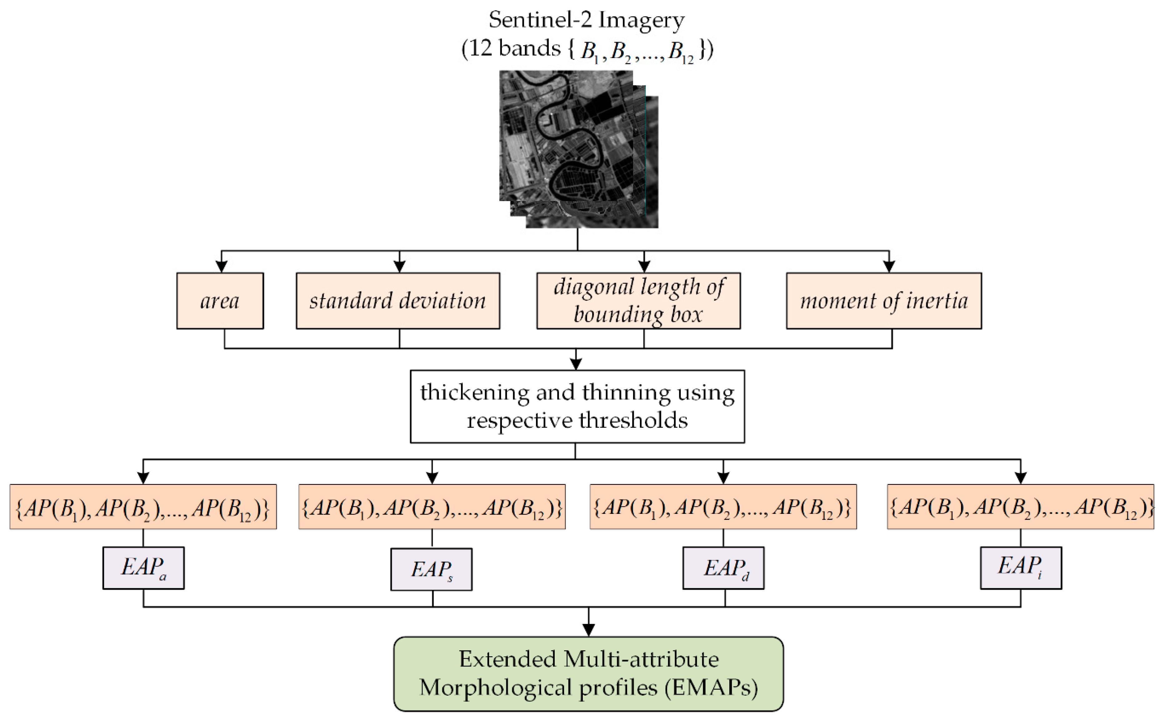In particular, extended multi-attribute profiles (EMAPs) [27,28,29] could present multilevel analysis for imagery via sequentially applying morphological attribute filters that are able to characterize the information in different object structures. As described, the construction of EMAPs avoids the requirement for predefined image structures. Moreover, it can keep the geometrical traits for relevant areas and effectively attenuate unimportant details [20,27,30], which is useful for preserving the boundaries of wetland regions and decreasing their within-class spectral and spatial variabilities.

Currently, machine learning is recognized as the most promising technique for quantitative information retrieval from remotely sensed images [31]. A series of machine learning approaches were developed, such as maximum likelihood (ML) [32], support vector machines (SVMs) [10,33], random forest (RF) [34,35], neural networks (NNs) [36], and so on. 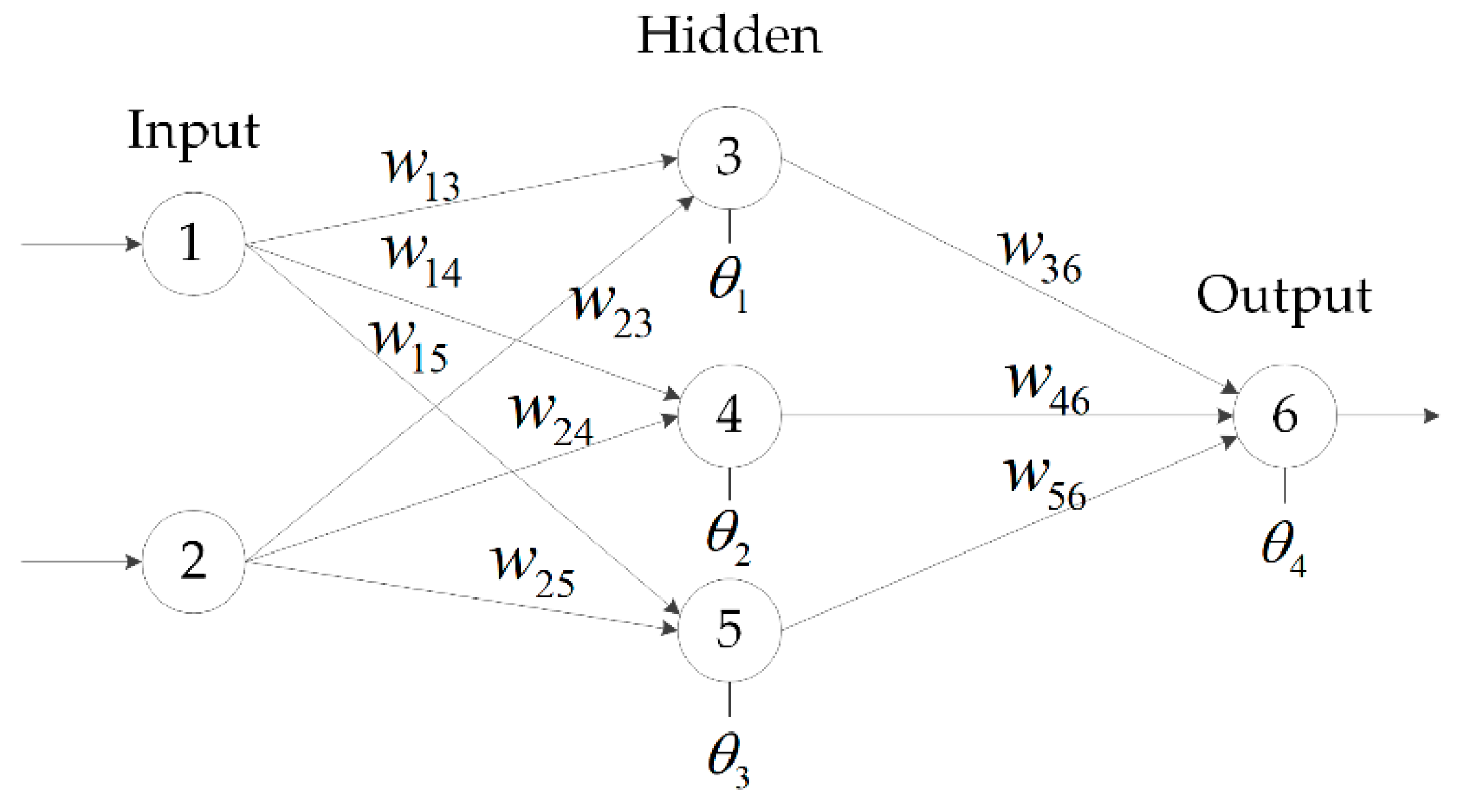Among the various machine learning methods, NN-based classifiers gain superiority in terms of robustness, high data error tolerance, and better classification performance [36,37,38]. When handling a complex dataset, multilayer perceptron (MLP) neural networks [39] are required, which feature more layers with a full connection between all neurons. As a typical nonparametric classifier, MLP is designed to learn the nonlinear features irrespective of their statistical properties, which is widely used in remotely sensed image processing [40,41,42] including coastal wetland classification [10,37,43]. Nevertheless, the estimation of parameters, such as weights and biases, in MLP is always a difficult task [44,45]. These parameters dramatically affect the trained model’s generalization capacity, as getting their optimal settings inevitably turns into a vital problem. In general, the error backpropagation algorithm (BP) [2,46] is utilized to train parameters weights and biases. This approach, on the other hand, easily falls into local optima and gets premature convergence [38,47]. In recent years, because of their promising self-organization and global optimization abilities, swarm intelligence algorithms, such as genetic algorithms (GAs) [40,48], particle swarm optimization (PSO) algorithms [46,49,50], and differential evolution (DE) [51] were successfully used to optimize the parameters of MLP.

Gravitational search algorithm (GSA) [52,53] is a recently developed swarm intelligence algorithm inspired by Newton’s law of gravity [54]. In GSA, agents are recognized as celestial bodies and search for the optimal solution via interactive movements under gravitational force. These years, GSA is increasingly popular because of its simple structure, well-understood theory, easily implemented strategy, and so on [55,56]. Nevertheless, GSA still faces a premature convergence problem when processing complicated problems [56,57,58,59]. Thus, many GSA variants were proposed [56,60], including the stability-constrained adaptive alpha for the gravitational search algorithm (SCAA) [61], in which the searching performance of GSA was improved by adaptively adjusting the important parameter alpha.

As the Sentinel-2 multispectral instrument (MSI) sensor simultaneously possesses rich spatial and spectral information, it shows enormous potential in characterizing wetland extents [9,62,63,64]. Researchers proposed many advanced techniques for mapping wetlands from Sentinel-2 images. Stratoulias et al. [9] mapped lakeshore areas using the selected high-spatial-resolution (i.e., 10 m and 20 m) bands of Sentinel-2 imagery on the basis of hyperspectral data and the satellite’s spectral response function. Chatziantoniou et al. [8] evaluated the performance of a synergistic utilization of Sentinel-1 and Sentinel-2 dataset for representing land use and land cover (LULC) of wetlands under SVMs. Therein, spectral features (gained from minimum noise fraction (MNF), principal component analysis (PCA)) and spatial features (GLCM texture, shape, and crop features) were extracted and employed on a complex wetland region. In Reference [65], an approach combining pixel-based, index-based, and object-based classification technique was introduced, in which NDVI and NDWI were employed for the discrimination of the contents within the wetlands, and an object-based method was used to extract the boundaries of wetland types. However, few of the methods tried utilizing the spatial information of Sentinel-2 imagery in multilevel to model the scale-varying objects in wetlands.

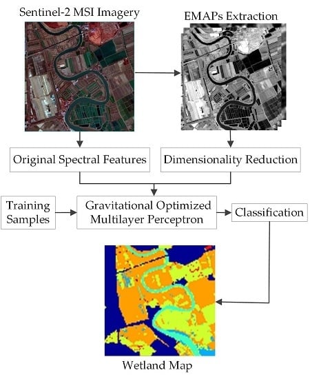
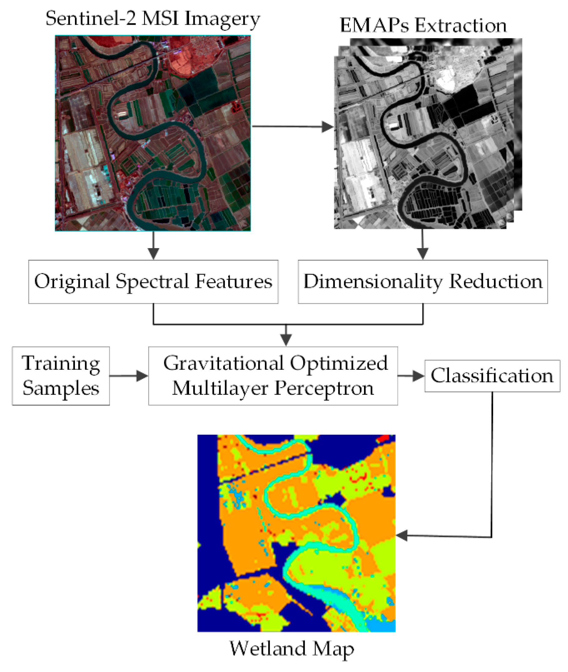
The overarching aim of this study was to propose a novel classification framework for Sentinel-2 MSI imagery of complex coastal wetlands by developing an optimized multilayer perceptron classifier and applying it to the spectral–spatial features constructed by the multispectral features and the EMAPs. The contributions of this research can be summarized as follows:

(1) Wetland EMAPs feature extraction: Four attribute filters are introduced based on the characteristics of wetlands in each band from Sentinel-2 imagery to extract the EMAPs that model the wetland objects in multiscale and multilevel.

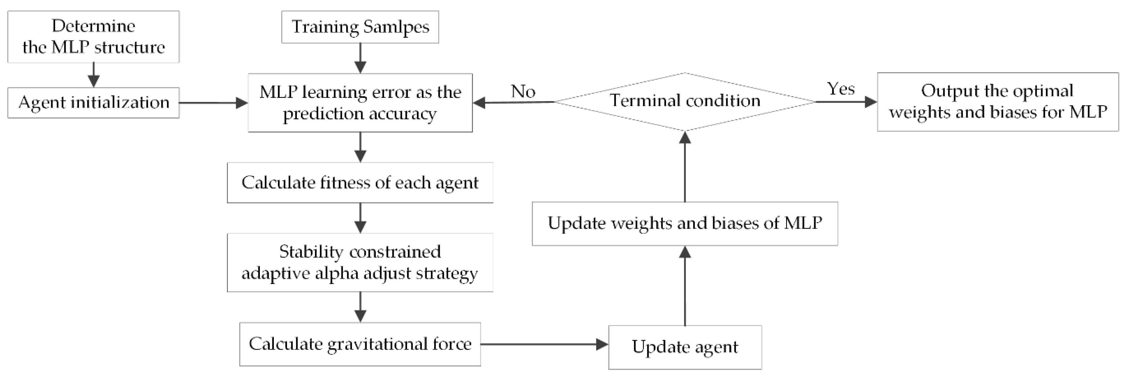
(2) A novel MLP classifier: The SCAA optimized MLP, which is denoted as SCAA_MLP, is proposed to select the most appropriate parameters of the MLP classifier. The superiority of SCAA in balancing exploration and exploitation can effectively promote the capability of MLP classifiers.

(3) Coastal wetland mapping: Through the application of SCAA_MLP classifier to the spectral and spatial features, accurate coastal wetland maps can be obtained.

The remainder of the paper is organized as follows: Section 2 gives a detailed introduction of the proposed method. Section 3 presents the studied areas and the experimental results. In Section 4, a careful discussion of the proposed method with some future scope is provided. Finally, Section 5 concludes the whole paper.

2. Methodology

The workflow of the proposed wetland mapping methodology is given in Figure 1, which includes the following three steps: EMAP feature extraction, MLP optimization by SCAA, and wetland classification via the proposed classifier. EMAPs of wetland are extracted using four attributes to describe different spatial properties of wetland objects. The novel MLP classifier is developed using SCAA and then applied for performing land-cover classification. More details about the proposed method are described in the following sections.

2.1. Wetland EMAP Feature Extraction

The coastal wetland scenes in study areas are complicated, and the spectra of wetland types have high between-class similarity and large within-class variation. Thus, it is difficult to classify wetland types merely depending on the spectral information. In recent years, the morphological attribute profile was applied as an effective spatial feature extraction tool, which performs a multilevel characterization of imagery to model various structural information. More importantly, using different attributes and multilevel operators, it can describe the multiscale and irregularly shaped wetland land covers. Furthermore, the attribute filter can effectively preserve the geometrical characteristics of objects and attenuate unimportant details [27]. Hence, it is useful to keep the boundaries of wetland types and decrease their within-class spectral and spatial variabilities. Therefore, in this paper, in addition to the original spectral band characteristics of wetlands, their spatial features in the form of morphological attribute profiles are constructed from Sentinel-2 imagery.

The EMAPs are obtained using different types of attributes on several grayscale images and stacking them together. Specifically, for a single grayscale image I, when the attribute is selected, the corresponding AP is achieved via applying a sequence of attribute thinning and thickening operators based on an ordered threshold {k₁, k₂, …, k_n} as follows [66]:

$$AP\left(I\right)=\left\{{\varphi }_{k_n}\left(I\right),{\varphi }_{k_{n-1}}\left(I\right),\dots ,{\varphi }_{k_1}\left(I\right),I,{\gamma }_{k_1}\left(I\right),\dots ,{\gamma }_{k_{n-1}}\left(I\right),{\gamma }_{k_n}\left(I\right)\right\}$$

(1)

where ${\varphi }_{k_n}(I)$ represents the filtered image generated via thickening operation ϕ with threshold k_n. A similar explanation is made for ${\gamma }_{k_n}\left(I\right)$. As a consequence, the number of images in the output $AP(I)$ is (2n + 1), which consists of the original grayscale image, n filtered images from thinning profiles, and the remaining n from thickening profiles.

Sentinel-2 imagery is a stack of grayscale images. In this research, we present attribute filtering operators on the full original spectral data (including 12 bands). That is, an extended attribute profile (EAP) is gained through producing an AP on each grayscale image of Sentinel-2 dataset S and then building a stacked vector.

$$EAP\left(S\right)=\left\{AP(B_1),AP(B_2),\dots ,AP(B_l)\right\}$$

(2)

where B_i is the ith band in the Sentinel-2 image and l is the number of bands.

To fully characterize the spatial features in the scene, different kinds of attributes are often applied [67]. These attributes are usually calculated with the geometric, spectral, or other characteristics of objects [24]. In this study, four attributes, area (region size), standard deviation (homogeneity of regions), diagonal length of bounding box, and moment of inertia (elongation of regions), are adopted. For the Sentinel-2 imagery S, as illustrated in Figure 2, its EMAPs are built with four attributes.

$$EMAP\left(S\right)=\left\{EA{P}_a(S),EA{P}_s(S),EA{P}_d(S),EA{P}_i(S)\right\}$$

(3)

where $EA{P}_a(S),EA{P}_s(S),EA{P}_d(S),EA{P}_i(S)$ are the EAPs for the image S considering the attributes area, standard deviation, diagonal length of bounding box, and moment of inertia, respectively.

The performance of the attribute filtering operation highly depends on its threshold value settings [29]. Due to the irregularly shaped and multiscale characteristics of wetland objects, selection of a proper threshold value can be a challenging task. A smaller value may introduce massive noise when processing large-sized heterogeneous wetland types, while a larger one could cause over-smoothness and erase some small useful information. In order to solve this issue, a threshold selection strategy according to previous studies [24] is utilized, which generates dense threshold values from a wide range. Therein, the filter thresholds of attributes area and standard deviation are set according to the characteristics of wetlands on Sentinel-2 datasets. As for the thresholds of area attribute k_a, each image resolution is considered as follows:

$$k_a\left(B_i\right)=\left(\frac{1000}{s{r}_i}\right)\times \left\{a_{\min },a_{\min }+{\delta }_a,a_{\min }+2{\delta }_a,\dots ,a_{\max }\right\}$$

(4)

where sr_i is the spatial resolution (in meters) of the ith band in Sentinel-2 imagery; $a_{\min }$ and $a_{\max }$ are set to 1 and 14, respectively, with an increasing step size ${\delta }_a$ equal to 1. As shown, due to the thresholds of each band being set according to its own spatial resolution, this method can better express the area information of ground objects in different resolution bands. The band with a high resolution (10 m) has more detailed information and the value of threshold is relatively small, which can be used to extract surface features with a small area. On the contrary, the larger threshold value corresponding to the low-resolution bands (20 m and 60 m) can be used to extract the contour information of large-area features.

The thresholds of standard deviation attribute k_s are adjusted based on the mean of the individual features as follows:

$$k_s\left(B_i\right)=\left(\frac{{\mu }_i}{100}\right)\times \left\{{\sigma }_{\min },{\sigma }_{\min }+{\delta }_s,{\sigma }_{\min }+2{\delta }_s,\dots ,{\sigma }_{\max }\right\}$$

(5)

where u_i denotes the average value of the ith band. The values of ${\sigma }_{\min }$, ${\sigma }_{\max }$, and ${\delta }_s$ are set to 2.5%, 27.5%, and 2.5%, respectively.

As for the diagonal length of bounding box attribute, its threshold values are varied between 10 and 100 with intervals equal to 10 (i.e., {10, 20, 30, 40, 50, 60, 70, 80, 90, 100}), whilst the filter thresholds of the moment of inertia attribute are selected from the range [0.1, 0.9] with intervals equal to 0.1 [33] (i.e., {0.1, 0.2, 0.3, 0.4, 0.5, 0.6, 0.7, 0.8, 0.9}). Accordingly, for the Sentinel 2 images with 12 bands, 1104 filtered images (including 348 for EAP_a, 276 for EAP_s, 228 for EAP_i, and 252 for EAP_d) can be obtained. In this context, the EMAPs are constructed with rich spatial information but inevitably possessing a large dimension and high redundancy. To reduce the computational burden, feature selection can be performed, for example, using the functions provided by the Weka (Waikato Environment for Knowledge Analysis) software [68].

2.2. Gravitational Optimized Multilayer Perceptron

Multilayer perceptron (MLP) is a commonly used neural network in remote sensing because of its relatively simple structure and higher classification capacity [36,69,70]. However, most traditional training methods usually fail to achieve proper parameters of MLP, i.e., weights and biases [38,51]. Recently, we proposed a new GSA variant, SCAA, to discourage its premature convergence problem [61]. It could balance the tradeoff between exploration and exploitation search, and realize stable convergence of swarm agents. Thus, it shows powerful potential in searching the optimal values of weights and biases in MLP, which can further improve the discrimination of complex wetland types. When applying SCAA to MLP, there are three key tasks that need to be addressed, i.e., the agent encoding, fitness function design, and swarm searching.

(A) Agent encoding strategy

A multilayer perceptron model usually has an input layer, one or more hidden layers, and an output layer, in which external information is imported into the input layer and results are obtained from the output layer. Figure 3 depicts a small instance of an MLP neural network with only one hidden layer, in which the number of neurons in the input layer is equal to two, that in the hidden layer is equal to three, and that in the output layer is equal to one. In MLP, neurons calculate the sum of entering data multiplied by a corresponding weight w at the presence of a bias θ; then, an activation function is applied to the sum and gained outcomes are transferred to the next layer.

In this study, the position vector of each agent ${\mathit{X}}_i=[x_{i1},\dots ,x_{id},\dots ,x_{iD}],\left(i=1,2,\dots ,NP\right)$ in a swarm is encoded as a possible solution of parameter combinations in MLP. In this way, the network is represented as a D-dimensional vector containing the possible parameters set of weights and biases, where D is defined as

$$D=(n_I\times n_H)+\left(n_H\times n_O\right)+n_H+n_O$$

(6)

where $n_I$, $n_H$ and $n_O$ are the numbers of neurons in the input, hidden, and output layers, respectively. Taking Figure 3 as an example, the corresponding encoding strategy is described as ${\mathit{X}}_i=[w_{13},w_{14},w_{15},w_{23},w_{24},w_{25},w_{36},w_{46},w_{56},{\theta }_1,{\theta }_2,{\theta }_3,{\theta }_4]$.

(B) Fitness function designing

The fitness value is an assessment for the performance of an agent. The agent with the best fitness value in swarm has a higher probability of finding the optimal solution (i.e., proper MLP parameter settings). Figure 4 simulates a neuron in MLP, the output of which in each learning period is computed according to Equations (7) and (8).

$$U_j={\displaystyle \sum _{i=1}^n{w}_{ji}{x}_j+{\theta }_j}$$

(7)

$$O_j=f_j\left(U_j\right)=\frac{1}{\left(1+e^{-U_j}\right)}$$

(8)

where w_ji is the connection weight between the ith and jth node, θ_j is the bias of the jth node, U_j represents the linear combination of input data, f (.) denotes the activation function, which is a sigmoid function in this study, and O_j is the obtained output of node j.

The network neurons perform such computations sequentially until all output results of neurons in output layer are achieved. Finally, the learning error is calculated as

$$MSE=\frac{1}{P}{{\displaystyle \sum _{k=1}^P\left(t_k-O_k\right)}}^2$$

(9)

where $t_k$ and $O_k$ denote the desired and actual outcomes of the MLP network, respectively, and P represents the quantity of neurons in the output layer.

The mean-square error (MSE) value is a measure of the accuracy of an MLP neural network. If an agent in swarm has a smaller MSE value, the weight and bias settings represented by it are more likely better. Hence, in this paper, the fitness function is designed as

$$fi{t}_i=MSE(X_i)$$

(10)

(C) Swarm search strategy

In SCAA, the gravitational constant attenuation factor alpha ($\alpha$), which takes an essential place in determining the gravitational force value, is dynamically adjusted by the adaptive alpha adjusting strategy and stability-based boundary constraint strategy. Therein, the evolutionary state of each agent in swarm is firstly evaluated and then utilized as feedback information to adaptively alter parameter $\alpha$. In addition, a boundary constraint for $\alpha$ is developed on the basis of GSA stability conditions to control the $\alpha$ value for the agents’ stable trajectories. In this context, the gravitational force is adaptively changed to achieve a better position vector of each agent. Figure 5 shows the flowchart of the swarm search strategy. The flowchart starts with defining the structure of the MLP, which includes the number of hidden layers and the quantity of neurons in each layer, to decide the agent vectors in SCAA. After that, the parameters of MLP are updated through the SCAA swarm search scheme, which is explained as follows:

Step 1: Initialize the population. Randomly initialize swarm agent vectors X in accordance with the following equation:

$$\mathit{X}=rand\left(NP,D\right)$$

(11)

where rand () could generate a series of random numbers in search space.

Step 2: Calculate the fitness value, i.e., the learning error of the MLP network encoded by the corresponding agent, using Equations (9) and (10).

Step 3: Use the stability-constrained adaptive alpha adjust strategy in SCAA to determine the value of parameter alpha for each agent.

Step 4: Calculate the gravitational force exerted on each agent according to its fitness value and parameter alpha.

Step 5: Update agent vectors. In this context, the new agent vector represents the updated settings of weights and biases in the MLP network.

Step 6: Exit the loop if the terminal condition is met and output the agent vector with the best fitness value, i.e., the optimal settings of weights and biases in MLP. Otherwise, go to step 2.

3. Experimental Results and Analysis

To investigate the performance of the proposed framework for coastal wetland classification, two important coastal wetlands in Shandong Province of eastern China were selected as study sites as shown in Figure 6 and introduced in Section 3.1. The detailed experimental settings are given Section 3.2. The classification accuracy of the SCAA_MLP for the two coastal wetlands is assessed through visual inspection and quantitative comparisons as presented in Section 3.3. In Section 3.4, we designed an experiment to evaluate the importance of EMAP spatial features in wetland discrimination.

3.1. Study Areas

The first coastal wetland is the Jiaozhou Bay wetland (35°58′–36°18′ north (N), 120°04′–120°23′ east (E)) situated on the southern coast of Shandong Peninsula and surrounded by a developing urban zone. Jiaozhou Bay is a semi-enclosed bay and opens an export to the Yellow Sea in the southeast direction. It has a prominent monsoon climate with 775.6 mm of mean annual precipitation and a 12.2 °C average annual temperature. More than 10 rivers and their tributaries, in which the largest one is Dagu River, run through this wetland region. One of the biggest ports in China, Qingdao Port, is posited in the eastern area. Jiaozhou Bay wetland supplies the breeding lands for various animals and plants, taking an important position for sea transportation, port construction, and the tourism industry [71]. However, Jiaozhou Bay wetland was gradually changed under anthropogenic activities because of the fast development of aquaculture, fish farming, transportation, and the tourism industry [1].

The second study site is the Yellow River Delta (YRD) wetland (37°33′–38°15′ N, 118°33′–119°22′ E). YRD wetland is located in the middle of the Bohai and Laizhou gulf, Dongying city in Shandong province. It is in the monsoon climate zone with 640 mm of mean annual precipitation, a 11.9 °C average annual temperature, and 1962 mm of average annual evaporation [72]. The adopted wetland scene in this work begins from Yuwa and ends at Songchunrong river in the south and Tiaohekou in the north. In recent years, two natural reserves, called Southern Nature Reserve (SNR) and Northern Nature Reserve (NNR), were authenticated by the national nature reserve and protection program in YRD wetland. Likewise, YRD wetland plays a vital role in breeding and wintering for many internationally considered rare water birds and fishes [73].

Sentinel datasets can be obtained from Copernicus Open Access Hub (https://scihub.copernicus.eu/). Two Sentinel-2A MSI L1C images used in this study were collected on 18 December 2017 (Jiaozhou Bay wetland) and 12 May 2016 (YRD wetland) under clear weather conditions. The data contained 13 bands ranging from the visible and near infrared (NIR) to the short-wavelength infrared (SWIR) spectral zone with various spatial resolutions, in which the resolution of three visible light (VIS) bands and one NIR band is 10 m, that of two SWIR and four vegetation red edge bands is 20 m, and that of one cirrus SWIR, one coastal aerosol, and one water vapor band is 60m. The directly acquired imagery from Copernicus Open Access Hub was Sentinel-2 level 1C data identified as a standard product of top-of-atmosphere reflectance values (TOA). Thus, in this paper, for the pre-processing step, particular atmospheric correction was required to transform TOA reflectance into corrected bottom-of-atmosphere reflectance values (BOA). Therefore, ESA’s Sen2Cor software was employed which could correct the Level 1C data in atmosphere, cirrus, and terrain to generate a Level 2A product. This operation would remove the 10th band from the dataset. After that, the remaining 12 bands in the imagery were resampled to 10 m via a bicubic method. Among these bands, although the resolutions of band 1 and band 9 were lower, they showed their efficiency in classification tasks, such as water body extraction [74], tropical coral reef mapping [75], and building shadow extraction [76].

The two study areas are surrounded by some downtown districts and suburban areas, in which wetland types are distributed sparsely and encompassed by built-up areas and vegetation. For the Jiaozhou Bay wetland and YRD wetland, seven wetland covers were found; they were identified as sea, tidal flat, river, breeding aquatics, saltern, reservoir pond, and vegetation. One more wetland type, paddy field, exists in the YRD study area. For reducing the computational cost in the further processing, the wetland mask was built manually with the reference of Google Earth and a field land cover survey to mask out the dry land regions in ENVI 5.3 software. For the selection of samples, to keep the correctness of samples, only identified land covers were adopted [36]. The samples with mixed pixels, such as in the sea boundaries, riverbanks, and sparse vegetation areas, were not taken into consideration. Moreover, for each site, both the Sentinel-2 imagery and the high-resolution images in Google Earth were utilized in the process of sample selection to further ensure the accuracy of the samples. The number of samples chosen for each wetland type is listed in

Table 1. Sample size for each wetland type in two study sites.

Jiaozhou Bay Wetland		Yellow River Delta Wetland
Wetland type	Size (pixels)	Wetland type	Size (pixels)
Sea	472,003	Sea	1,785,869
Tidal flat	79,122	Tidal flat	673,730
River	28,406	River	311,428
Breeding aquatics	80,197	Breeding aquatics	503,059
Saltern	32,277	Saltern	104,574
Reservoir pond	68,683	Reservoir pond	376,751
Vegetation	6920	Paddy field	146,753
		Vegetation	339,302

.

3.2. Design of Experiments

To evaluate the performance of SCAA_MLP, four advanced machine learning classifiers, SVM [33], RF [35], BP-trained MLP (denoted as BP_MLP) [36], and GSA-optimized MLP (denoted as GSA_MLP) [53], were applied in the wetland classification with the same input features for thorough comparison. As for the parameter settings, in RF, the value of Ntree was set to 500 for stable errors [77], which was commonly used in majority of the studies [35]. For BP_MLP, we tested the architecture with one, two, and four hidden layers and a varying number of {4, 8, 10, 12, 16, 20, 24, 30} nodes on the image of Jiaozhou Bay wetland. The corresponding overall accuracy (OA) and kappa coefficients (κ) were adopted to quantitatively estimate the setting of parameters. When the number of hidden layers was set to 1, the accuracy of BP_MLP could not be improved obviously with the number of neurons increased and could not achieve lower accuracy (OA of around 68%). When setting two hidden layers, its OA increased with the number of nodes rising from four to 30, whereas it kept stable and did not improve (OA of around 71%) with the number of nodes more than 16. Meanwhile, the time cost grew with the increase in the number of layers. For the BP_MLP with four hidden layers, when the numbers of nodes in the first three layers were set to 30, 30, and 30, and the number of nodes in the fourth layer was larger than 10, the accuracy was stable (with OA equal to 72%). Due to more nodes requiring more computation time, for balancing the efficiency and accuracy, four hidden layers with 30, 30, 30, and 10 nodes in each layer were adopted. Following the recommendations in Reference [32], the structures of GSA_MLP and SCAA_MLP neural networks were tested, and the optimal structure was found to have two hidden layers with 20 neurons in each layer. The parameter configurations of these classifiers are summarized in

Table 2. Parameter configurations of different classifiers. SVM—support vector machine; RF—random forest; BP—backpropagation; MLP—multilayer perceptron; GSA—gravitational search algorithm; SCAA—stability-constrained adaptive alpha.

Classifier	Parameter Description	Parameter Value
SVMs	Kernel type	Gaussian radial basis function (RBF)
	Gamma in the kernel function	0.143
	Penalty parameter	100
RF	Number of decision trees	500
	Number of considered variables	Square root of the number of input features
BP_MLP	Number of hidden layers	4
	Number of nodes in the first three hidden layers	30
	Number of neurons in the fourth hidden layers	10
	Learning rate	0.001
	Training epochs	1000
GSA_MLP	Number of hidden layers	2
	Number of nodes in the hidden layers	20
	Training epochs	1000
	Gravitational constant attenuation factor alpha	7
	Gravitational constant	50
SCAA_MLP	Number of hidden layers	2
	Number of nodes in the hidden layers	20
	Training epochs	1000
	Gravitational constant	50
	Limit value lp	4
	The maximum of attenuation factor alpha	7

.

According to Section 2.1, the EMAP features with four attributes were constructed containing 1104 filtered images to represent the spatial information of the Sentinel-2 dataset. To realize the dimensionality reduction of EMAPs, the information gain-based method [78] was used for feature selection, and a ranked list was generated to show superior attributes. This step was conducted using the well-known software Weka [68]. Consequently, the dimensionality of EMAPs was reduced from 1104 to 60.

For each run, the samples were randomly divided into three parts: 40% for training, 10% for validation, and 50% for testing, to ensure no overlapping between these data. The same samples were employed for all five classification methods. In order to quantitatively estimate the classification accuracy, the confusion matrix was calculated according to the testing data and classification results of the five classifiers in each scene. Based on the error matrix, we could obtain the overall accuracy (OA) and kappa coefficients (κ). The overall accuracy describes the proportion of the number of correctly identified points in the total testing data. The kappa value is defined as the percentage of accurately classified testing points after removing random agreement. For a fair comparison, all involved methods were carried out using Matlab 2017b on a computer with an Intel (R) Xeon (R) central processing unit (CPU) (1.70 GHz) and 32 GB of memory.

3.3. Classification Results and Analysis

In this section, the performance of SCAA_MLP and other comparative classifiers was tested on two coastal wetland study sites. Note that all classifiers were input the same features (12 spectral features and 60 EMAP spatial features). To provide a better visualization, the best results among different classifiers in quantitative comparison are marked in bold face, whilst correct or incorrect parts in classification maps are highlighted in black or magenta circles, respectively.

(1) Study site 1: Jiaozhou Bay wetland

The quantitative classification accuracy assessment in the first study scene is summarized in

Table 3. The classification accuracy of different classifiers in Jiaozhou Bay wetland. OA—overall accuracy.

Type	SVM	RF	BP_MLP	GSA_MLP	SCAA_MLP
Sea	99.96	97.6734	69.75	86.07	95.07
Tidal flat	97.22	90.1495	93.33	75.02	95.92
River	4.57	95.0683	60.55	59.82	90.40
Breeding aquatics	73.33	80.3641	46.70	44.48	94.39
Saltern	66.30	89.2085	91.02	98.07	97.53
Reservoir pond	12.99	91.6535	89.29	9.80	95.61
Vegetation	62.76	88.7848	97.78	83.29	98.06
OA	84.51	94.51	72.16	73.4935	95.09
κ	0.6922	0.8905	0.5844	0.5438	0.9171

. As shown, the proposed SCAA_MLP classifier achieved desirable classification results compared with other methods. To be specific, the SCAA_MLP gained the highest overall accuracy (95.09%) and kappa coefficient (κ) value (0.9171), dramatically higher than the MLP variants, BP_MLP (OA of 72.16% and κ of 0.5844) and the GSA_MLP (OA of 73.4935% and κ of 0.5438). This result was also superior when compared with other machine learning approaches, including SVM (84.51% OA and κ of 0.6922) and RF (94.51% OA and κ of 0.8905). Its promising performance was further validated through the per-class classification accuracy. When compared with BP_MLP, the classification accuracies of river and breeding aquatics grew dramatically by 48.7% and 102%, respectively. A slight rise of 36.3% was obtained for the sea classification. Other wetland types (tidal flat, saltern, reservoir pond, vegetation, etc.) marginally increased with respect to mapping precision (less than 1.5%). This is mainly because the effective search strategy in SCAA achieves better weight and bias settings in MLP, which facilitates the discrimination of complex nonlinear wetland features. In comparison with other machine learning methods, the higher classification results of the proposed SCAA_MLP were validated in the classes of breeding aquatics, reservoir pond, and vegetation, with a per-class mapping accuracy of 94.39%, 95.61%, and 98.06%, respectively. As for sea, river, and saltern, however, SCAA_MLP was inferior to SVM and RF, with a slight accuracy decrease. In general, the quantitative classification results demonstrated that SCAA_MLP achieved a superior performance for complex Jiaozhou Bay wetland types.

The effectiveness of SCAA_MLP was also validated by visual inspection. To provide a useful visualization, the classification images of Jiaozhou Bay wetland obtained by different classifiers are presented in Figure 7. As a whole, SCAA_MLP obtained the smoothest visual results with accurate boundary information and high geometric fidelity compared with its peers. Most importantly, as shown in Figure 7f, the wetland types with similar spectral information (e.g., river, reservoir pond, sea, etc.) and land covers with great within-object variation (e.g., breeding aquatics and dry parts in river channels due to the variation in water volume and vegetation density) were effectively characterized. With regard to other classifiers, in the classification map obtained by SVM and GSA_MLP (Figure 7b,e), the linearly shaped features like river were misclassified as sea and reservoir pond, whilst simple wetland categories like reservoir pond were wrongly identified as sea (see the regions marked by magenta circles). For the highly complex land covers with great intra-class heterogeneity, for example, some parts of breeding aquatics, they were wrongly distinguished as river by BP_MLP and GSA_MLP. In addition, in the dry river channel, SVM, RF, BP_MLP, and GSA_MLP failed to capture the sparse vegetation and misclassified the detailed thin river. However, all classifiers performed worse along the edges between sea and tidal flat. Some areas in tidal flat were recognized as breeding aquatics by SVM, RF, and BP_MLP (marked by magenta circles in Figure 7b–d), while parts of sea regions were classified as reservoir pond by all methods, especially BP_MLP and GSA_MLP. This is mainly due to the high spectral and spatial confusion in this area, which lacks precise training samples for classifiers due to the challenges in visual interpretation. Fortunately, most features were correctly distinguished by SCAA_MLP without losing useful information as depicted in Figure 7f. These results are consistent with the quantitative classification accuracy evaluation.

(2) Study site 2: Yellow River Delta wetland

The quantitative classification accuracy of different classifiers on the second study site is illustrated in

Table 4. The classification accuracy of different classifiers in Yellow River Delta wetland.

Type	SVM	RF	BP_MLP	GSA_MLP	SCAA_MLP
Sea	90.20	97.40	83.22	96.05	97.95
Tidal flat	55.25	93.33	83.56	89.34	97.27
River	77.06	91.91	80.30	0	88.33
Breeding aquatics	3.70	88.08	32.54	59.03	90.74
Saltern	41.10	90.30	81.43	87.57	91.72
Reservoir pond	28.66	92.11	62.38	80.61	93.19
Paddy field	84.69	97.79	96.37	95.80	98.62
Vegetation	95.56	98.50	98.35	98.60	98.87
OA	67.09	94.73	76.82	82.19	95.81
κ	0.5326	0.9320	0.6997	0.7624	0.9450

. From the results, it is obvious that the highest mapping precision was also obtained by SCAA_MLP with an OA of 95.81% and a kappa coefficient (κ) value of 0.9450, markedly higher than SVM (OA of 67.09% and κ of 0.5326), BP_MLP (OA of 76.82% with κ of 0.6997), and GSA_MLP (OA of 82.19% and κ of 0.7624). The superiority of SCAA_MLP was further demonstrated by the per-classification accuracy. When compared with BP_MLP, the classification accuracies of breeding aquatics, reservoir pond, sea, tidal flat, saltern, and river were dramatically increased by 64.14%, 33.06%, 15.03%, 14.09%, 11.22%, and 9.09%, respectively. Such a rise in classification accuracy can also be validated in Figure 8d,f. The breeding aquatics in YRD wetland have higher within-class variation due to the water volume difference and bare wet soil existence. Despite the utilization of EMAP features, BP_MLP failed to capture breeding aquatics correctly and mostly misclassified them as tidal flat (marked in magenta circles). Due to the saline alkali areas in tidal flat, these regions were wrong recognized as saltern by BP_MLP. Furthermore, there was considerable misclassification between reservoir pond, sea, and river as shown by magenta circles in Figure 8d. This is mainly because the BP algorithm is easily trapped into local optima, which causes MLP to lack the capacity in processing complex spectral and spatial information of objects. From Table 4, the employment of GSA could facilitate this issue to some extent, in which the mapping accuracy of most wetland types were moderately increased. However, GSA_MLP failed to capture the linear-shaped river features as depicted in Figure 8e. In contrast, since SCAA further improved the optimization performance of GSA, these undesirable visual effects and misclassifications were rectified significantly. From Figure 8, we can see that SCAA_MLP also achieved the smoothest classification map on YRD wetland with higher geometric fidelity and more precise edges between classes, which confirms its universality on complex wetland mapping. Different from the other approaches, SVM also performed worse in the second experiment despite various spatial and spectral features being used.

3.4. Effectiveness of EMAPs

For assessing the effectiveness of EMAP features, two tests were carried out using datasets in Jiaozhou Bay wetland and YRD wetland. Specifically, the significance of spatial features produced by different attribute profiles was tested using SCAA_MLP with spectral information of 12 bands in Sentinel-2 imagery and spectral–spatial features generated by adding EAP_s, EAP_a, EAP_d, EAP_i, and EMAPs. The results on two study sites including per-class classification accuracy, overall accuracy (OA), and kappa coefficient (κ) are reported in

Table 5. Classification accuracy obtained using spectral and different spectral–spatial features (Jiaozhou Bay wetland). EAP—extended attribute profile; EMAP—extended multi-attribute profile.

Type	Spectral Features	Spectral EAPa	Spectral EAPs	Spectral EAPd	Spectral EAPi	Spectral EMAPs
Sea	91.05	92.78	92.14	93.53	95.00	95.07
Tidal flat	94.28	96.15	93.36	96.53	93.48	95.92
River	77.67	87.61	76.24	87.28	85.52	90.40
Breeding aquatics	75.55	83.89	67.89	94.10	81.92	94.39
Saltern	96.23	96.69	96.57	98.24	97.44	97.53
Reservoir pond	86.32	88.05	87.96	90.91	88.53	95.61
Vegetation	94.95	96.63	98.49	94.69	93.55	98.06
OA	89.13	91.79	89.06	93.64	92.69	95.09
κ	0.8197	0.8630	0.8181	0.8935	0.8766	0.9171

and

Table 6. Classification accuracy obtained by using spectral and different spectral–spatial features (Yellow River Delta (YRD) wetland).

Type	Spectral Features	Spectral EAPa	Spectral EAPs	Spectral EAPd	Spectral EAPi	Spectral EMAPs
Sea	91.68	96.93	95.04	96.91	96.30	97.95
Tidal flat	95.16	97.36	95.60	94.66	98.31	97.27
River	89.96	88.80	89.57	88.19	94.33	88.33
Breeding aquatics	85.61	93.80	85.33	93.66	92.17	90.74
Saltern	92.04	94.27	95.99	96.50	92.57	91.72
Reservoir pond	90.23	95.22	88.42	96.67	87.67	93.19
Paddy field	96.36	98.83	97.65	98.90	98.84	98.62
Vegetation	98.79	99.16	99.41	99.36	99.20	98.87
OA	91.99	95.55	93.45	95.76	95.45	95.81
κ	0.8963	0.9491	0.9147	0.9446	0.9405	0.9450

, respectively. The best results are highlighted in bold face.

With respect to the Jiaozhou Bay wetland, as shown in Table 5, it is clear that combining spatial information from EMAPs with original spectral information largely improved the classification accuracy, which was higher than only using spectral features. Specifically, the EAP_a features improved the OA to 91.79% and κ to 0.8630. This may come from the area attributes extracted based on the spatial resolution information of Sentinel-2 images, which can better express the area information of ground objects in different resolution bands. Similar results were gained by integrating the EAP_i measures. Much higher accuracy was reported by adding the EAP_d information, achieving an overall accuracy of 93.64% with a kappa value of 0.8935. However, the utilization of feature EAP_s degraded the classification performance. Thus, for mapping Jiaozhou Bay wetland, EAP_s was abandoned in this paper and the EMAP consisting of EAP_a, EAP_d, and EAP_i was employed as the spatial information. As shown in Table 5, combining these measures with the original spectral layers obtained the best accuracy, achieving an OA of 95.09% with κ of 0.9171. From the per-class classification accuracy, it is obvious that EAP_d (i.e., the attribute diagonal length of bounding box) was effective in the identification of squarely shaped objects, such as breeding aquatics, saltern, and reservoir pond. For the linear river, the attribute area contributed more than other attributes.

The classification maps of the Jiaozhou Bay wetland obtained by SCAA_MLP adopting 12 spectral features and spectral EMAP spatial features are depicted in Figure 9b,c, respectively. Based on the visual inspection, it can clearly be seen that, when replying purely upon spectral features, the mapping results consisted of undesirable noise (highlighted in magenta circles), especially for the mapping of wetland types with higher within-object variation (e.g., river) and the boundary areas. At the same time, the classes with similar spectral characteristics (e.g., river, reservoir pond, breeding aquatics, sea etc.) had a higher tendency to be misclassified (magenta circles in Figure 9b). For instance, some edge regions along the sea and several parts in wide river area were wrongly distinguished as reservoir pond, while breeding aquatics and dry river channel areas were not accurately mapped. On the contrary, with the addition of the EMAP spatial features, as represented in Figure 9c, certain improvements were achieved in both spectral and spatial pattern differentiation, which exhibited smoothed visual effects with little noise. This is mainly due to the fact that EMAPs can preserve the geometrical features of objects and attenuate unimportant details. Thus, it can suppress noise and keep precise boundaries. In addition, the utilization of different attributes and multilevel operators made the best of spatial characteristics of wetland regions, which realized the correct discrimination of objects with similar spectral features.

As for the YRD wetland, from Table 6, it is clear that the spectral–spatial based classification via adding different EAPs achieved higher accuracy at all points than only employing spectral information. Specifically, SCAA_MLP achieved a worse overall accuracy of 91.99% merely considering 12 original spectral features. However, when utilizing the spectral–spatial features by adding EAP_a, EAP_s, EAP_d, EAP_i, and EMAPs, its OA was 95.55%, 93.45%, 95.76%, 95.45%, and 95.81%, respectively. Similar to the first experiment, it is clear that, amongst the four constructed EAPs, using EAP_d allowed achieving higher OA, especially in the discrimination of saltern, reservoir pond, and paddy field. Thus, for square regions in the two study sites, the attribute diagonal length of bounding box can provide better spatial description than other attributes. By contrast, in the YRD wetland study area, EAP_i (i.e., moment of inertia attribute) performed best for the classification of linearly shaped objects, like river.

As for the visualization shown in Figure 10, similar to the test in Jiaozhou Bay wetland, the employment of EMAP features enabled SCAA achieving smoother wetland classification with less noise. For example, the small speckles in sea and tidal flat (magenta circles in Figure 10b) were much reduced in Figure 10c. Additionally, the misclassifications between sea, river, and reservoir pond, and between saltern and tidal flat (highlighted by magenta circles), which appeared in Figure 10b, were revised accordingly.

The test outcomes illustrated that EMAPs were effective in relieving the between-class homogeneity and within-class heterogeneity for complex wetland classification, with the EAP_a, EAP_d, and EAP_i measures contributing more. More importantly, the combination of the selected EAPs with the spectral layers achieved superior results compared to combining any single EAP measure, which more fully described the spatial features of wetlands.

4. Discussion

Coastal wetland types in Setinel-2 remotely sensed imagery are highly complex with low within-class homogeneity and between-class heterogeneity. Merely relying on the spectral characteristics of wetlands results in massive misclassification and noise. As depicted in Figure 9b and Figure 10b, confusion appeared among spectral similar objects like river, reservoir pond, breeding aquatics, and sea, while severe noise existed in the heterogeneous wetland types like river and breeding aquatics. The boundary information between different wetland objects was also weakened with the blurred classification. These issues demonstrate the need for using effective spatial features of coastal wetlands. The proposed method in this paper incorporates EMAPs as a spatial characterization tool. The utilization of different attributes and dense filter threshold settings provides multilevel spatial description modeling various structural information in the irregularly shaped wetland types. Moreover, the attribute filter operation can preserve the geometrical characteristics of objects and attenuate unimportant details, for they do not need to predefine image structures. In this context, the utilization of EMAPs is helpful to decrease intra-class variability, improve inter-class variability, and delineate boundaries. This superiority was validated by the quantitative analysis (Table 5 and Table 6) and visual inspection (Figure 9c and Figure 10c), whereby spectrally similar wetland types (e.g., river, reservoir pond, sea, etc.) and greatly heterogeneous objects (e.g., breeding aquatics, sparse vegetation, and dry river channel areas) were correctly classified with less noise and accurate boundaries.

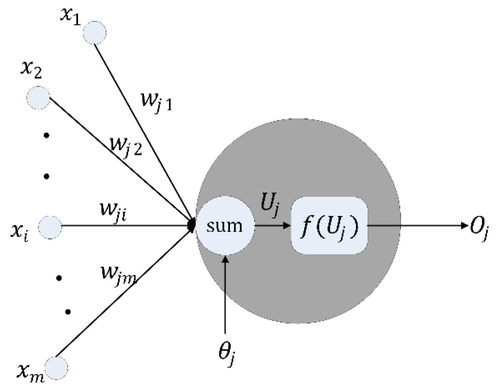
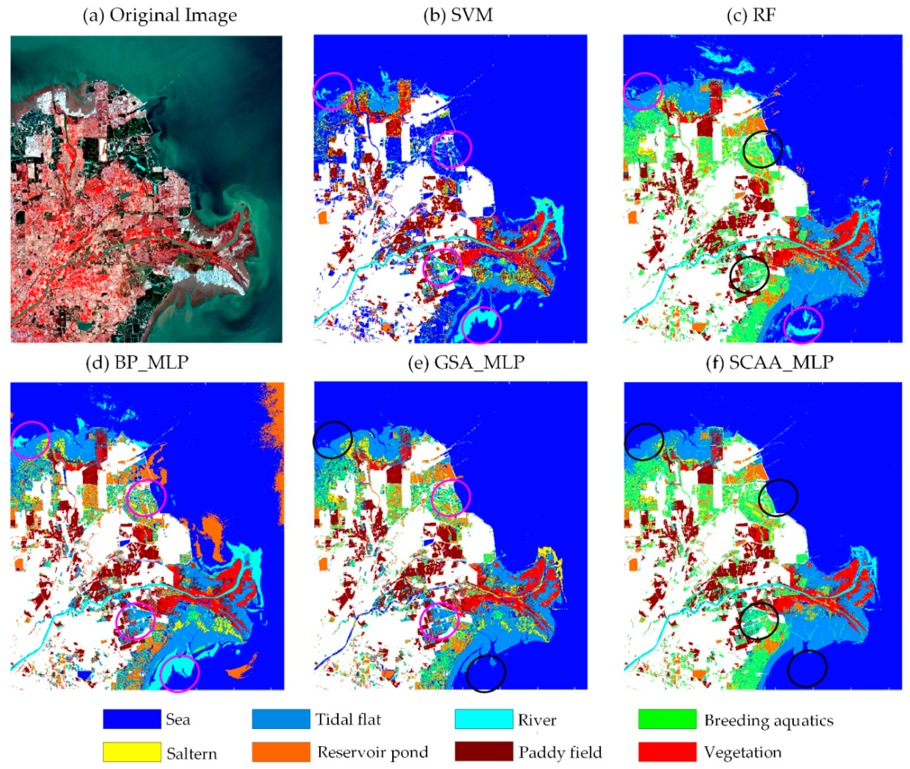
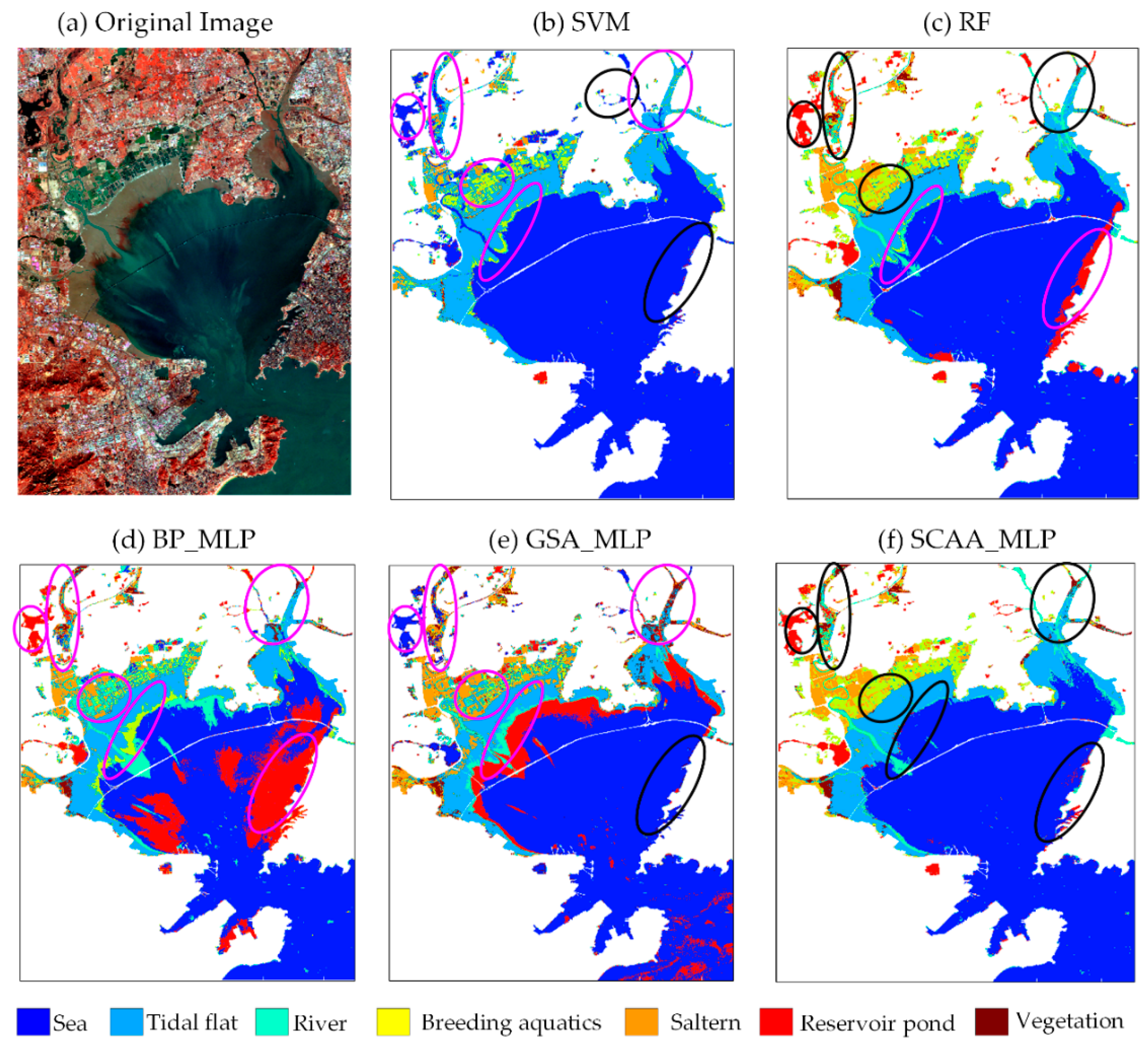
In MLP neural networks, the input of each neuron is firstly weighted and bias is added, and then it is handled by a nonlinear activation function. During this process, the performance of MLP significantly relies on the parameter weight and bias settings. However, traditional training approaches tend to fall into local optima and fail to obtain the optimal values for weights and biases [38,47]. Such limitations usually cause undesirable classification results; for instance, misclassification and confusion between the river, reservoir pond, breeding aquatics, and sea that are spectrally similar appeared in the coastal wetland classification maps of BP_MLP and GSA_MLP despite the employment of EMAP spatial features. Even for those correctly identified objects, some noise still existed, as presented in Figure 7d,e and Figure 8d,e. In this work, the intelligent optimization algorithm SCAA, which achieves superior balance between exploration and exploitation search to escape from local optima, was used to effectively set proper values of weights and biases in MLP. The classification results in Table 3 and Table 4 suggest that SCAA_MLP achieved desirable results in terms of OA and per-class classification accuracy. In addition, from Figure 7f and Figure 8f, SCAA_MLP achieved the smoothest classification maps on Jiaozhou Bay wetland and YRD wetland with precise boundary information and high geometric fidelity.

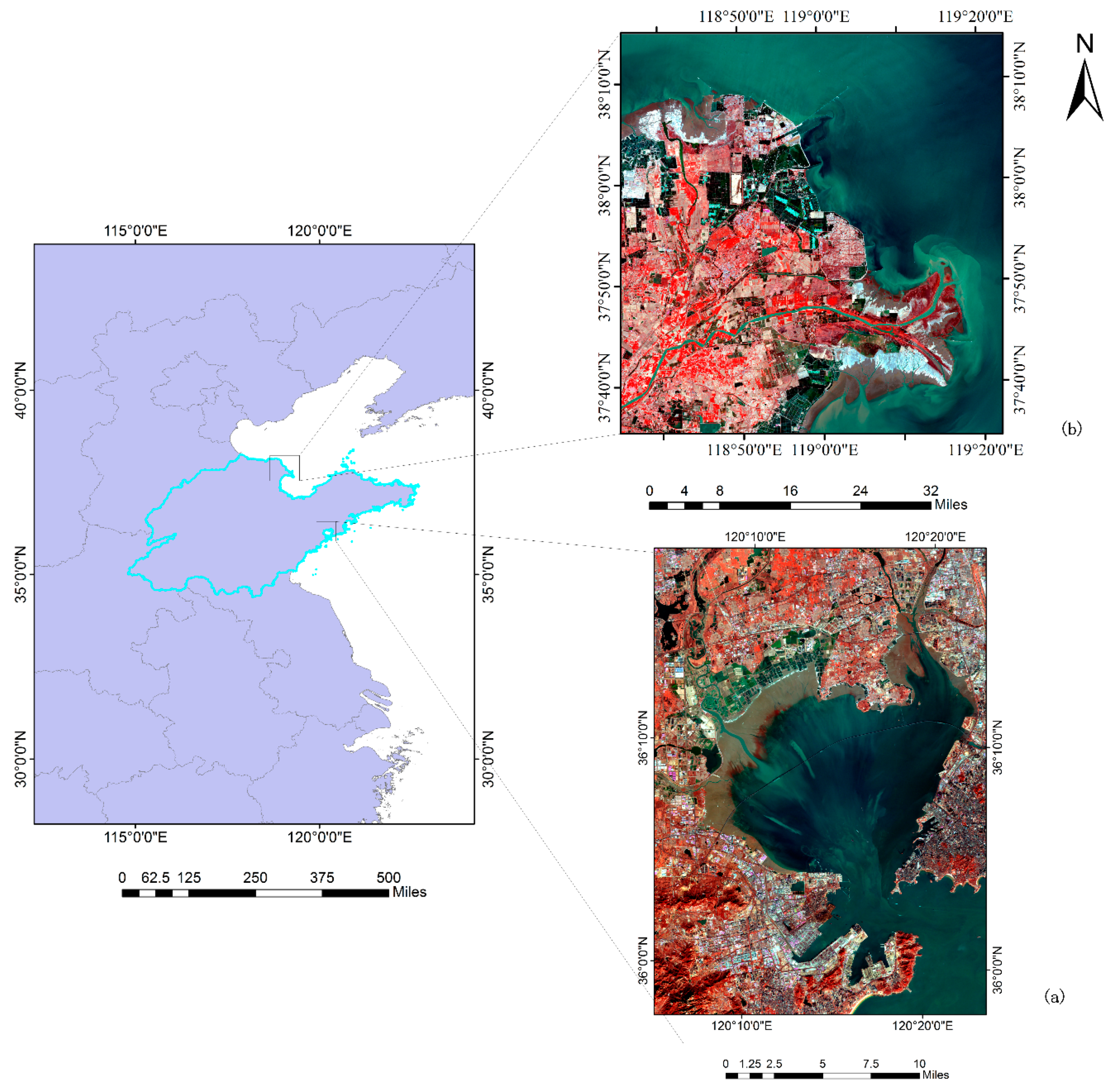
From the classification maps in Section 4, it is clear that most coastal wetland types in Jiaozhou Bay and Yellow River Delta can be roughly divided into natural wetlands and artificial wetlands. In Jiaozhou Bay, the artificial wetlands, like some reservoir ponds, breeding aquatics, and salterns, are mainly found in the northern and northwestern regions with regular shapes. In the Yellow River Delta, artificial wetland types are mainly distributed on the northern, northeastern, and eastern coasts, in which paddy fields are identified in northern and central parts. Moreover, the Yellow River Delta coastal wetlands are characterized by extensive salinization, especially in the tidal flat, which leads to the misclassification with saltern. These factors indicate the strong relationship between regional industrial and agricultural development and land cover distribution in the coastal zone. As a special ecosystem, coastal wetland is vulnerable to alteration and shrinkage due to natural fluctuations and external disturbance. In a future study, a multitemporal remotely sensed dataset on Jiaozhou Bay wetland and YRD wetland will be utilized to analyze the dynamic change of different wetland types. Furthermore, the relative significance of natural and anthropogenic variables in the observed wetland changes will be assessed and evaluated to reveal the impact of environmental conditions on wetland change.

5. Conclusions

In this research, we proposed a novel spectral–spatial classification framework for coastal wetland using Sentinel-2 remotely sensed imagery, in which morphological attribute profiles (APs) were extracted and a multilayer perceptron (MLP) classifier was optimized by SCAA. This framework aimed to identify the different coastal wetland classes with high within-class variability and low between-class disparity. For comprehensively employing spectral and spatial information, large EMAPs were built considering four different attributes, area, standard deviation, moment of inertia, and diagonal length of bounding box, with their filter thresholds sampled in small intervals from a wide range based on the characteristics of wetland types on Sentinel-2 imagery. These features can provide multilevel spatial descriptions of irregularly shaped wetland objects and they can decrease intra-class variability via attribute filter operation. To process the complex spectral and spatial information of coastal wetlands, a new MLP classifier was developed, in which three tasks including an agent encoding strategy, a fitness function designing, and a SCAA swarm search scheme were utilized. By using the superiority of SCAA in balancing exploration and exploitation, the optimal values of parameter weight and bias in MLP were obtained. Experimental results on the Sentinel-2 MSI images of Jiaozhou Bay wetland and Yellow River Delta wetland confirmed the effectiveness of the proposed method. It is anticipated that this work could boost the application of Sentinel-2 imagery in global coastal wetland mapping and monitoring, and accordingly promote the research of coastal wetland ecosystems.

References

1. Gu, D.; Zhang, Y.; Fu, J.; Zhang, X. The landscape pattern characteristics of coastal wetlands in Jiaozhou Bay under the impact of human activities. Environ. Monit. Assess 2007, 124, 361–370. [Google Scholar] [CrossRef]
2. Li, L.; Chen, Y.; Xu, T.; Liu, R.; Shi, K.; Huang, C. Super-resolution mapping of wetland inundation from remote sensing imagery based on integration of back-propagation neural network and genetic algorithm. Remote Sens. Environ. 2015, 164, 142–154. [Google Scholar] [CrossRef]
3. Jiang, Y.; Wang, Y.; Liao, M.; Zhang, L. Study of coastal wetland classification based on decision rules using ALOS AVNIR-2 images and ancillary geospatial data. Geocarto Int. 2015, 30, 1172–1188. [Google Scholar] [CrossRef]
4. Dong, Z.; Wang, Z.; Liu, D.; Song, K.; Li, L.; Jia, M.; Ding, Z. Mapping wetland areas using landsat-derived NDVI and LSWI: A case study of west Songnen Plain, Northeast China. J. Indian Soc. Remote Sens. 2014, 42, 569–576. [Google Scholar] [CrossRef]
5. Cazals, C.; Rapinel, S.; Frison, P.-L.; Bonis, A.; Mercier, G.; Mallet, C.; Corgne, S.; Rudant, J.-P. Mapping and characterization of hydrological dynamics in a coastal marsh using high temporal resolution Sentinel-1A images. Remote Sens. 2016, 8, 570. [Google Scholar] [CrossRef]
6. Chen, Y.; He, X.; Wang, J.; Xiao, R. The influence of polarimetric parameters and an object-based approach on land cover classification in coastal wetlands. Remote Sens. 2014, 6, 12575–12592. [Google Scholar] [CrossRef]
7. Bansal, S.; Katyal, D.; Garg, J.K. A novel strategy for wetland area extraction using multispectral MODIS data. Remote Sens. Environ. 2017, 200, 183–205. [Google Scholar] [CrossRef]
8. Chatziantoniou, A.; Psomiadis, E.; Petropoulos, G. Co-orbital Sentinel 1 and 2 for LULC mapping with emphasis on wetlands in a mediterranean setting based on machine learning. Remote Sens. 2017, 9, 1259. [Google Scholar] [CrossRef]
9. Stratoulias, D.; Balzter, H.; Sykioti, O.; Zlinszky, A.; Toth, V.R. Evaluating Sentinel-2 for lakeshore habitat mapping based on airborne hyperspectral data. Sensors 2015, 15, 22956–22969. [Google Scholar] [CrossRef] [PubMed]
10. Zhang, C.; Xie, Z. Combining object-based texture measures with a neural network for vegetation mapping in the Everglades from hyperspectral imagery. Remote Sens. Environ. 2012, 124, 310–320. [Google Scholar] [CrossRef]
11. Ashraf, M.; Nawaz, R. A Comparison of change detection analyses using different band algebras for Baraila wetland with NASA’s multi-temporal landsat dataset. J. Geogr. Inf. Syst. 2015, 7, 1–19. [Google Scholar] [CrossRef]
12. Spencer, T.; Schuerch, M.; Nicholls, R.J.; Hinkel, J.; Lincke, D.; Vafeidis, A.T.; Reef, R.; Mcfadden, L.; Brown, S. Global coastal wetland change under sea-level rise and related stresses: The DIVA Wetland Change Model. Glob. Planet. Chang. 2016, 139, 15–30. [Google Scholar] [CrossRef] [Green Version]
13. Rogers, K.; Saintilan, N.; Woodroffe, C.D. Surface elevation change and vegetation distribution dynamics in a subtropical coastal wetland: Implications for coastal wetland response to climate change. Estuar. Coast. Shelf Sci. 2014, 149, 46–56. [Google Scholar] [CrossRef]
14. Cline, M.D.; Feagin, R.A.; Yeager, K.M.; Alstyne, J.M.V. Fault-induced wetland loss at Matagorda, Texas, USA: Land cover changes from 1943 to 2008. Geocarto Int. 2011, 26, 633–645. [Google Scholar] [CrossRef]
15. Demarchi, L.; Canters, F.; Cariou, C.; Licciardi, G.; Chan, J.C.-W. Assessing the performance of two unsupervised dimensionality reduction techniques on hyperspectral APEX data for high resolution urban land-cover mapping. ISPRS J. Photogramm. 2014, 87, 166–179. [Google Scholar] [CrossRef]
16. Prigent, C.; Papa, F.; Aires, F.; Jimenez, C.; Rossow, W.B.; Matthews, E. Changes in land surface water dynamics since the 1990s and relation to population pressure. Geophys. Res. Lett. 2012, 39, 85–93. [Google Scholar] [CrossRef]
17. Ghamisi, P.; Mura, M.D.; Benediktsson, J.A. A survey on spectral-spatial classification techniques based on attribute profiles. Ieee Trans. Geosci. Remote Sens. 2015, 53, 2335–2353. [Google Scholar] [CrossRef]
18. Lane, C.; Liu, H.; Autrey, B.; Anenkhonov, O.; Chepinoga, V.; Wu, Q. Improved wetland classification using eight-band high resolution satellite imagery and a hybrid approach. Remote Sens. 2014, 6, 12187–12216. [Google Scholar] [CrossRef]
19. Wu, Y.; Wang, C.; Yu, L.; Zhang, D. Using MRF approach to wetland classification of high spatial resolution remote sensing imagery: A case study in Xixi Westland National Park, Hangzhou, China. In Proceedings of the Second Iita International Conference on Geoscience and Remote Sensing, Qingdao, China, 28–31 August 2010. [Google Scholar] [CrossRef]
20. Demir, B.; Bruzzone, L. Histogram-based attribute profiles for classification of very high resolution remote sensing images. Ieee Trans. Geosci. Remote Sens. 2016, 54, 2096–2107. [Google Scholar] [CrossRef]
21. Herold, M.; Liu, X.H.; Clarke, K.C. Spatial metrics and image texture for mapping urban land use. Photogramm. Eng. Remote Sens. 2003, 69, 991–1002. [Google Scholar] [CrossRef]
22. Zhang, C.; Sargent, I.; Pan, X.; Li, H.; Gardiner, A.; Hare, J.; Atkinson, P.M. An object-based convolutional neural network (OCNN) for urban land use classification. Remote Sens. Environ. 2018, 216, 57–70. [Google Scholar] [CrossRef]
23. Fauvel, M.; Tarabalka, Y.; Benediktsson, J.A.; Chanussot, J.; Tilton, J.C. Advances in spectral-spatial classification of hyperspectral images. Proc. IEEE 2013, 101, 652–675. [Google Scholar] [CrossRef]
24. Ghamisi, P.; Benediktsson, J.A.; Cavallaro, G.; Plaza, A. Automatic framework for spectral–spatial classification based on supervised feature extraction and morphological attribute profiles. IEEE J. Sel. Top. Appl. Earth Obs. Remote Sens. 2014, 7, 2147–2160. [Google Scholar] [CrossRef]
25. Bhardwaj, K.; Patra, S. An unsupervised technique for optimal feature selection in attribute profiles for spectral-spatial classification of hyperspectral images. ISPRS J. Photogramm. 2018, 138, 139–150. [Google Scholar] [CrossRef]
26. Khodadadzadeh, M.; Li, J.; Prasad, S.; Plaza, A. Fusion of hyperspectral and LiDAR remote sensing data using multiple feature learning. IEEE J. Sel. Top. Appl. Earth Obs. Remote Sens. 2017, 8, 2971–2983. [Google Scholar] [CrossRef]
27. Falco, N.; Mura, M.D.; Bovolo, F.; Benediktsson, J.A.; Bruzzone, L. Change detection in VHR images based on morphological attribute profiles. IEEE Geosci. Remote Sens. Lett. 2013, 10, 636–640. [Google Scholar] [CrossRef]
28. Benediktsson, J.A.; Bruzzone, L.; Chanussot, J.; Mura, M.D.; Salembier, P.; Valero, S. Hierarchical analysis of remote sensing data: morphological attribute profiles and binary partition trees. In Proceedings of the International Conference on Mathematical Morphology and its Applications to Image and Signal Processing, Verbania-Intra, Italy, 6–8 July 2011. [Google Scholar] [CrossRef]
29. Song, B.; Li, J.; Mura, M.D.; Li, P.; Plaza, A.; Bioucas-Dias, J.M.; Benediktsson, J.A.; Chanussot, J. Remotely Sensed Image Classification Using Sparse Representations of Morphological Attribute Profiles. IEEE Trans. Geosci. Remote Sens. 2014, 52, 5122–5136. [Google Scholar] [CrossRef] [Green Version]
30. Song, B.; Li, J.; Li, P.; Plaza, A. Decision fusion based on extended multi-attribute profiles for hyperspectral image classification. In Proceedings of the Workshop on Hyperspectral Image & Signal Processing: Evolution in Remote Sensing, Gainesville, FL, USA, 26–28 June 2013. [Google Scholar] [CrossRef]
31. Zhang, C.; Pan, X.; Li, H.; Gardiner, A.; Sargent, I.; Hare, J.; Atkinson, P.M. A hybrid MLP-CNN classifier for very fine resolution remotely sensed image classification. ISPRS J. Photogramm. 2018, 140, 133–144. [Google Scholar] [CrossRef]
32. Yang, F.; Guo, J.; Tan, H.; Wang, J. Automated Extraction of Urban Water Bodies from ZY-3 Multi-Spectral Imagery. Water 2017, 9, 144. [Google Scholar] [CrossRef]
33. Ghamisi, P.; Couceiro, M.S.; Benediktsson, J.A. A Novel Feature Selection Approach Based on FODPSO and SVM. IEEE Trans. Geosci. Remote Sens. 2015, 53, 2935–2947. [Google Scholar] [CrossRef] [Green Version]
34. Berhane, T.M.; Lane, C.R.; Wu, Q.; Anenkhonov, O.A.; Chepinoga, V.V.; Autrey, B.C.; Liu, H. Comparing Pixel- and Object-Based Approaches in Effectively Classifying Wetland-Dominated Landscapes. Remote Sens. 2018, 10, 46. [Google Scholar] [CrossRef] [PubMed]
35. Belgiu, M.; Drăguţ, L. Random forest in remote sensing: A review of applications and future directions. ISPRS J. Photogramm. Remote Sens. 2016, 114, 24–31. [Google Scholar] [CrossRef]
36. Jiang, W.; He, G.; Long, T.; Ni, Y.; Liu, H.; Peng, Y.; Lv, K.; Wang, G. Multilayer Perceptron Neural Network for Surface Water Extraction in Landsat 8 OLI Satellite Images. Remote Sens. 2018, 10, 755. [Google Scholar] [CrossRef]
37. Bao, Y.; Ren, J. Wetland Landscape Classification Based on the BP Neural Network in DaLinor Lake Area. Procedia Environ. Sci. 2011, 10, 2360–2366. [Google Scholar] [CrossRef] [Green Version]
38. Ren, C.; An, N.; Wang, J.; Li, L.; Hu, B.; Shang, D. Optimal parameters selection for BP neural network based on particle swarm optimization: A case study of wind speed forecasting. Knowl. Based Syst. 2014, 56, 226–239. [Google Scholar] [CrossRef]
39. Taravat, A.; Proud, S.; Peronaci, S.; Del Frate, F.; Oppelt, N. Multilayer Perceptron Neural Networks Model for Meteosat Second Generation SEVIRI Daytime Cloud Masking. Remote Sens. 2015, 7, 1529–1539. [Google Scholar] [CrossRef] [Green Version]
40. Liu, Z.; Liu, A.; Wang, C.; Niu, Z. Evolving neural network using real coded genetic algorithm (GA) for multispectral image classification. Future Gener. Comp. Sy 2004, 20, 1119–1129. [Google Scholar] [CrossRef]
41. Toshniwal, M. An optimized approach to application of neural networks to classification of multispectral, remote sensing data. In Proceedings of the Networking, Sensing and Control Proceedings, Tucson, AZ, USA, 19–22 March 2005. [Google Scholar] [CrossRef]
42. Yuan, H.; Van Der Wiele, C.; Khorram, S. An Automated Artificial Neural Network System for Land Use/Land Cover Classification from Landsat TM Imagery. Remote Sens. 2009, 1, 243–265. [Google Scholar] [CrossRef] [Green Version]
43. Zun-You, K.; Ru, A.; Xiang-Juan, L. ANN Based High Spatial Resolution Remote Sensing Wetland Classification. In Proceedings of the 2015 14th International Symposium on Distributed Computing and Applications for Business Engineering and Science (DCABES), Guiyang, China, 18–24 August 2015; pp. 180–183. [Google Scholar] [CrossRef]
44. Mirjalili, S.; Mirjalili, S.M.; Lewis, A. Let a biogeography-based optimizer train your Multi-Layer Perceptron. Inf. Sci. 2014, 269, 188–209. [Google Scholar] [CrossRef]
45. Mirjalili, S. How effective is the Grey Wolf optimizer in training multi-layer perceptrons. Appl. Intell. 2015, 43, 150–161. [Google Scholar] [CrossRef]
46. Xu, J.; Yang, Y.; Zhang, R. Graduate enrollment prediction by an error back propagation algorithm based on the multi-experiential particle swarm optimization. In Proceedings of the International Conference on Natural Computation, Zhangjiajie, China, 15–17 August 2015. [Google Scholar] [CrossRef]
47. Lian, C.; Zeng, Z.; Yao, W.; Tang, H.; Chen, C.L. Landslide Displacement Prediction With Uncertainty Based on Neural Networks With Random Hidden Weights. IEEE Trans. Neural Netw. Learn. Syst. 2016. [Google Scholar] [CrossRef]
48. Sheikhpour, S.; Sabouri, M.; Zahiri, S.H. A hybrid gravitational search algorithm-genetic algorithm for neural network training. In Proceedings of the Electr Eng, Mashhad, Iran, 14–16 May 2013. [Google Scholar] [CrossRef]
49. Beheshti, Z.; Shamsuddin, S.M.H.; Beheshti, E.; Yuhaniz, S.S. Enhancement of artificial neural network learning using centripetal accelerated particle swarm optimization for medical diseases diagnosis. Soft Comput. 2014, 18, 2253–2270. [Google Scholar] [CrossRef]
50. Rakitianskaia, A.S.; Engelbrecht, A.P. Training feedforward neural networks with dynamic particle swarm optimisation. Swarm Intell. 2012, 6, 233–270. [Google Scholar] [CrossRef] [Green Version]
51. Pratimsarangi, P.; Sahu, A.; Panda, M. A Hybrid Differential Evolution and Back-Propagation Algorithm for Feedforward Neural Network Training. Int. J. Comput. Appl. 2014, 1–9. [Google Scholar] [CrossRef]
52. González, B.; Valdez, F.; Melin, P.; Prado-Arechiga, G. Fuzzy logic in the gravitational search algorithm for the optimization of modular neural networks in pattern recognition. Expert Syst. Appl. 2015, 42, 5839–5847. [Google Scholar] [CrossRef]
53. Mirjalili, S.; Hashim, S.Z.M.; Sardroudi, H.M. Training feedforward neural networks using hybrid particle swarm optimization and gravitational search algorithm. Appl. Math. Comput. 2012, 218, 11125–11137. [Google Scholar] [CrossRef]
54. Rashedi, E.; Nezamabadi-Pour, H.; Saryazdi, S. GSA: A Gravitational Search Algorithm. Inf. Sci. 2009, 179, 2232–2248. [Google Scholar] [CrossRef]
55. Jiang, S.; Wang, Y.; Ji, Z. Convergence analysis and performance of an improved gravitational search algorithm. Appl. Soft Comput. 2014, 24, 363–384. [Google Scholar] [CrossRef]
56. Gao, S.; Vairappan, C.; Wang, Y.; Cao, Q.; Tang, Z. Gravitational search algorithm combined with chaos for unconstrained numerical optimization. Appl. Math. Comput. 2014, 231, 48–62. [Google Scholar] [CrossRef]
57. Zhang, N.; Li, C.; Li, R.; Lai, X.; Zhang, Y. A mixed-strategy based gravitational search algorithm for parameter identification of hydraulic turbine governing system. Know. Based Syst. 2016. [Google Scholar] [CrossRef]
58. Li, C.; Chang, L.; Huang, Z.; Liu, Y.; Zhang, N. Parameter identification of a nonlinear model of hydraulic turbine governing system with an elastic water hammer based on a modified gravitational search algorithm. Eng. Appl. Artif. Intel. 2016, 50, 177–191. [Google Scholar] [CrossRef]
59. Zhang, A.; Sun, G.; Ren, J.; Li, X.; Wang, Z.; Jia, X. A Dynamic Neighborhood Learning-Based Gravitational Search Algorithm. IEEE Trans. Cybern. 2016, 1–12. [Google Scholar] [CrossRef]
60. Mirjalili, S.; Lewis, A. Adaptive gbest-guided gravitational search algorithm. Neural Comput. Appl. 2014, 25, 1569–1584. [Google Scholar] [CrossRef]
61. Sun, G.; Ma, P.; Ren, J.; Zhang, A.; Jia, X. A stability constrained adaptive alpha for gravitational search algorithm. Knowl. Based Syst. 2018, 139, 200–213. [Google Scholar] [CrossRef]
62. Yang, X.; Zhao, S.; Qin, X.; Zhao, N.; Liang, L. Mapping of Urban Surface Water Bodies from Sentinel-2 MSI Imagery at 10 m Resolution via NDWI-Based Image Sharpening. Remote Sens. 2017, 9, 596. [Google Scholar] [CrossRef]
63. Clerici, N.; Calderón, C.A.V.; Posada, J.M. Fusion of Sentinel-1A and Sentinel-2A data for land cover mapping: A case study in the lower Magdalena region, Colombia. J. Maps 2018, 13, 718–726. [Google Scholar] [CrossRef]
64. Amani, M.; Salehi, B.; Mahdavi, S.; Granger, J. Spectral analysis of wetlands in newfoundland using Sentinel 2A and Landsat 8 imagery. In Proceedings of the ASPRS Conference, Baltimore, MA, USA, 26–28 March 2013. [Google Scholar] [CrossRef]
65. Kaplan, G.; Avdan, U. Mapping and monitoring wetlands using Sentinel-2 satellite imagery. ISPRS Ann. Photogramm. Remote Sens. Spat. Inf. Sci. 2017, 271–277. [Google Scholar] [CrossRef]
66. Pham, M.-T.; Lefèvre, S.; Merciol, F. Attribute profiles on derived textural features for highly textured optical image classification. IEEE Geosci. Remote Sens. Lett. 2018. [Google Scholar] [CrossRef]
67. Urbach, E.R.; Roerdink, J.B.; Wilkinson, M.H. Connected shape-size pattern spectra for rotation and scale-invariant classification of gray-scale images. IEEE Trans. Pattern Anal. Mach. Intell. 2007, 29, 272–285. [Google Scholar] [CrossRef] [PubMed]
68. Yadav, A.K.; Malik, H.; Chandel, S.S. Selection of most relevant input parameters using WEKA for artificial neural network based solar radiation prediction models. Renew. Sust. Energ. Rev. 2014, 31, 509–519. [Google Scholar] [CrossRef]
69. Czyzowska-Wisniewski, E.H.; van Leeuwen, W.J.D.; Hirschboeck, K.K.; Marsh, S.E.; Wisniewski, W.T. Fractional snow cover estimation in complex alpine-forested environments using an artificial neural network. Remote Sens. Environ. 2015, 156, 403–417. [Google Scholar] [CrossRef]
70. Li, X.; Song, W.; Lian, L.; Wei, X. Forest Fire Smoke Detection Using Back-Propagation Neural Network Based on MODIS Data. Remote Sens. 2015, 7, 4473–4498. [Google Scholar] [CrossRef] [Green Version]
71. Zhang, J.; Sun, Y. Eco-environmental Quality and Ecological Restoration: A case study in wetland of the loushan river estuary, Jiaozhou Bay, Qingdao. In Proceedings of the International Workshop on Education Technology and Training & 2008 International Workshop on Geoscience and Remote Sensing, Shanghai, China, 21–22 December 2008. [Google Scholar] [CrossRef]
72. Liu, G.; Zhang, L.; Zhang, Q.; Musyimi, Z.; Jiang, Q. Spatio–Temporal Dynamics of Wetland Landscape Patterns Based on Remote Sensing in Yellow River Delta, China. Wetlands 2014, 34, 787–801. [Google Scholar] [CrossRef]
73. Zhang, H.; Chen, X.; Luo, Y. An overview of ecohydrology of the Yellow River delta wetland. Ecohydrol. Hydrobiol. 2016, 16, 39–44. [Google Scholar] [CrossRef] [Green Version]
74. Kaplan, G.; Avdan, U. Object-based water body extraction model using sentinel-2 satellite imagery. Eur. J. Remote Sens. 2017, 50, 137–143. [Google Scholar] [CrossRef]
75. Hedley, J.; Roelfsema, C.; Koetz, B.; Phinn, S. Capability of the sentinel 2 mission for tropical coral reef mapping and coral bleaching detection. Remote Sens. Environ. 2012, 120, 145–155. [Google Scholar] [CrossRef]
76. Sun, G.; Huang, H.; Weng, Q.; Zhang, A.; Jia, X.; Ren, J.; Sun, L.; Chen, X. Combinational shadow index for building shadow extraction in urban areas from sentinel-2a msi imagery. Int. J. Appl. Earth Obs. Geoinf. 2019, 78, 53–65. [Google Scholar] [CrossRef]
77. Lawrence, R.L.; Wood, S.D.; Sheley, R.L. Mapping invasive plants using hyperspectral imagery and Breiman Cutler classifications (randomForest). Remote Sens. Environ. 2006, 99, 356–362. [Google Scholar] [CrossRef]
78. Russell, I.; Markov, Z. An introduction to the Weka data mining system. In Proceedings of the 2017 Sigcse Conference on Innovation & Technical Symposium on Computer Science Education (SIGCSE), Washington, DC, USA, 8–11 March 2017. [Google Scholar] [CrossRef]
Figure 1. Flowchart of coastal wetland mapping from Sentinel-2 multispectral instrument (MSI) imagery.
Remotesensing 11 00952 g001
Figure 2. General scheme of constructing an extended attribute profile (EAP) from Sentinel-2 imagery. The extended multi-attribute profile (EMAP) is a combination of EAPs generated with four different attributes.
Remotesensing 11 00952 g002
Figure 3. A small example of a multilayer perceptron (MLP) with a 2–3–1 structure.
Remotesensing 11 00952 g003
Figure 4. A neuron of an MLP [50].
Remotesensing 11 00952 g004
Figure 5. Flowchart of stability-constrained adaptive alpha (SCAA) optimizing MLP.
Remotesensing 11 00952 g005
Figure 6. The study areas: (a) Jiaozhou Bay wetland and (b) Yellow River Delta (YRD) wetland (satellite images from Sentinel-2 are shown in false color red–green–blue (RGB) = near-infrared (NIR)–red–green).
Remotesensing 11 00952 g006
Figure 7. Classification results in Jiaozhou Bay wetland, with (a) an image subset (NIR, G, and B bands only), (b) support vector machine (SVM) classification, (c) random forest (RF) classification, (d) MLP classification, (e) gravitational search algorithm (GSA)–MLP classification, and (f) SCAA_MLP classification.
Remotesensing 11 00952 g007
Figure 8. Classification results in Yellow River Delta wetland, with (a) an image subset (NIR, G, and B bands only), (b) SVM classification, (c) RF classification, (d) MLP classification, (e) GSA_MLP classification, and (f) SCAA_MLP classification.
Remotesensing 11 00952 g008
Figure 9. Classification results in Jiaozhou Bay wetland with (a) an image subset (NIR, G, and B bands only), (b) SCAA_MLP classification with spectral features, and (c) SCAA_MLP classification with spectral EMAP spatial features.
Remotesensing 11 00952 g009
Figure 10. Classification results in Yellow River Delta (YRD) wetland, with (a) an image subset (NIR, G, and B bands only), (b) SCAA_MLP classification with spectral features, and (c) SCAA_MLP classification with spectral EMAP features.
Remotesensing 11 00952 g010