Quantification and Analysis of Impervious Surface Area in the Metropolitan Region of São Paulo, Brazil

Abstract

The growing intensity of impervious surface area (ISA) is one of the most striking effects of urban growth. The expansion of ISA gives rise to a set of changes on the physical environment, impacting the quality of life of the human population as well as the dynamics of fauna and flora. Hence, due to its importance, the present study aimed to examine the ISA distribution in the Metropolitan Region of São Paulo (MRSP), Brazil, using satellite imagery from the Landsat-8 Operational Land Imager (OLI) instrument. In contrast to other investigations that primarily focus on the accuracy of the estimate, the proposal of this study is—besides generating a robust estimate—to perform an integrated analysis of the impervious-surface distribution at pixel scale with the variability present in different territorial units, namely municipalities, sub-prefecture and districts. The importance of this study is that it strengthens the use of information related to impervious cover in the territorial planning, providing elements for a better understanding and connection with other spatial attributes. Reducing the dimensionality of the dataset (visible, near-infrared and short-wave infrared bands) by Karhune–Loeve analysis, the first three principal components (PCs) contained more than 99% of the information present in the original bands. Projecting PC1, PC2 and PC3 onto a series of two-dimensional (2D) scatterplots, four endmembers—Low Albedo (Dark), High Albedo (Substrate), Green Vegetation (GV) and Non-Photosynthetic Vegetation (NPV)—were visually selected to produce the unmixing estimates. The selected endmembers fitted the model well, as the propagated error was consistently low (root-mean-square error = 0.005) and the fraction estimates at pixel scale were found to be in accordance with the physical structures of the landscape. The impervious surface fraction (ISF) was calculated by adding the Dark and Substrate fraction imagery. Reconciling the ISF with reference samples revealed the estimates to be reliable (R² = 0.97), regardless of an underestimation error (~8% on average) having been found, mostly over areas with higher imperviousness rates. Intra-pixel variability was combined with the territorial units of analysis through a modification of the Lorenz curve, which permitted a straightforward comparison of ISF values at different reference scales. Good adherence was observed when the original 30-m ISF was compared to a resampled 300-m ISF, but with some differences, suggesting a systematic behavior with the degradation of pixel resolution tending to underestimate lower fractions and overestimate higher ones; furthermore, discrepancies were bridged with the increase of scale analysis. The analysis of the IFS model also revealed that, in the context of the MRSP, gross domestic product (GDP) has little potential for explaining the distribution of impervious areas on the municipality scale. Finally, the ISF model was found to be more sensitive in describing impervious surface response than other well-known indices, such as Normalized Difference Vegetation Index (NDVI) and Normalized Difference Built-up Index (NDBI).

1. Introduction

In the strict sense, impervious surface area (ISA) corresponds to areas where soil infiltration by water is impeded, mainly due to imperviousness resulting from anthropogenic interventions in the landscape, such as buildings, driveways, paved streets, parking lots, etc. Besides being considered an important element of urbanization, ISA has a close relationship with important characteristics of the physical and biological environment, affecting the quality and maintenance of life.

In urban areas, one of the most notorious impacts of the increase in ISA is the increase in velocity and volume of runoff, which potentially increases the scale and frequency of flooding [1,2,3]. Another prominent change concerns the increase in latent and sensible heat flux. Urban materials, such as asphalt, concrete and asbestos, have a capacity to absorb more solar energy, which is then released as heat. As a consequence, a strong positive correlation is found when impervious surface values are plotted against the temperature of the environment [4,5,6,7]. Deterioration of water quality also relates to sprawling ISA [8,9], with deleterious impacts on fauna and flora [10].

Studies conducted by Schueler [8] revealed that, in many hydrographic basins, environmental degradation occurs at a relatively low level of soil imperviousness of just 10–20%. Impervious coverage thus scales up the transport of nutrients (N and K), toxic contaminants and pathogenic agents to rivers, streams and lakes. A global inventory of the spatial distribution and density of ISA [11] indicates that watersheds damaged by ISA are primarily concentrated in the USA, Europe, Japan, China and India. On the other hand, pristine watersheds having little or no ISA are concentrated in central Asia, portions of Africa, the Amazon Basin and the southern regions of South America and the Arabian Peninsula.

An increase in ISA is associated with the intensification of economic activities in the secondary and tertiary sectors. However, this relationship is not linearly distributed in space and time. Once a given locality diversifies its economy, ISA usually increases rapidly as the infrastructure necessary for that development is created. From a certain stage of growth, when the essential infrastructure is already in place, the ISA variability starts to depend on other attributes, such as the presence of vegetation in the urban plot and the spatial arrangement set in the urban planning. Guo et al. [12] conducted an interesting study relating the economic conditions of Chinese cities with the root-mean-square (RMS) error generated from the ISA estimates. They concluded that gross domestic product (GDP) is an important factor affecting the estimation errors. Considering the example of Beijing and Shanghai, the two largest populations and GDPs in China, the study highlighted the fact that the highest estimation errors found in these cities were related to their distinct characteristics in spatial patterns of urban landscapes and different land-coverage compositions.

Remote sensing constitutes the main source of data for mapping and monitoring ISA [13,14,15]. Indeed, one of the biggest challenges in mapping ISA using optical remote sensing is to deal with the great spectral diversity of impervious materials that compose the urban plots [16,17]. Industrial rooftops usually present a high reflectance of energy that is commonly confused with bright soils; on the other hand, paved roads and old tiles have significantly lower reflectance values that often mimic the spectral signatures of flooded areas, rivers or shade [18]. To some extent, this explains the difficulties found in mapping ISA accurately.

To determine the extent of ISA, most studies have used visual interpretation or automatic image-classification techniques [3,19,20,21]. Despite producing accurate results, visual interpretation of high-resolution aerial photography, for instance, has the drawback of being subjective, time consuming and not practical over large areas. On the other hand, the applicability of running an automatic classification in aerial photography or orbital imagery depends on several factors, such as the characteristics of the algorithm being used, the combination of bands employed, and the physical nature of the study area under analysis [21].

The image-classification task is even more difficult in urban areas due to the heterogeneity of land use in a relatively small space, which amplifies the problem of the pixel-mixing effect. The spectral-mixing effect occurs when a given pixel registers the energy signal coming from two or more targets or materials on the surface. Therefore, the intensity of the mixing effect basically depends on the spatial configuration of the land use (extrinsic factor) and the spatial resolution of the image (intrinsic factor). In urban areas, only a few pixels are pure. The preponderance of mixed pixels registered in Landsat imagery (30 m) occurs due to the decorrelation of urban reflectance observed at 10–20 m [22]. Even in higher spatial-resolution imagery, such as the Ikonos multispectral images (4 m), the proportion of mixed pixels found in the image is quite significant [23]. For statistical classification, mixed pixels are problematic because most algorithms are predicated on the assumption of spectral homogeneity within a particular land class. When this assumption is violated, statistical classification can fail to appropriately represent land information.

In order to circumvent the problems related to the spectral-mixing effect, techniques that privilege intra-pixel variability in their analysis should be adopted. One of the most effective techniques designed to manage the matter of the mixing effect is the spectral mixture analysis (SMA) [24]. SMA provides valuable information on the physical components of the landscape by taking into consideration the relative presence of dominant spectral materials signalized at pixel level. In addition to enhancing targets of interest, the use of the mixing analysis has the advantage of simplifying the interpretation of the images [24,25], given that interpreting an image in terms of approximate fractions of the different materials present in each pixel is easier than considering the values expressed in terms of the radiance, reflectance or emittance of the materials.

SMA constitutes one of the primary techniques used in a variety of disciplines. Investigations related to rock and soil [26,27], forest [25,28,29,30], burning severity [31,32], land-use and land-cover mapping [33,34,35] and urban applications [16,36,37,38,39], as well as specific analyses related to ISA [5,13,15,18,23,40,41,42,43] are just a few examples of applications.

Due to the importance that ISA imposes on the environment, this study aimed at mapping the ISA distribution in the Metropolitan Region of São Paulo (MRSP), southeastern Brazil. Most studies addressed to ISA have focused on the process of estimating and minimizing the errors associated with it. Our research has gone beyond this scope. In addition to delineating a robust model for impervious surface fraction (ISF) in terms of accurate estimates, we also propose analyzing, in a simple but efficient way, the behavior of impervious surface distribution, bridging the variability found within the pixel with the variability present in the territorial units. The importance of this study is that it strengthens the use of information related to ISF in territorial planning, providing elements for a better understanding and connection with other attributes in space. Hence, to perform this study, multispectral imagery taken from the Landsat-8 Operational Land Imager (OLI) instrument was used. The choice of the Landsat imagery is based on its ready availability and global distribution; however, other data, such as those collected by Sentinel, may also be employed using the methodology described.

2. Materials and Methods

2.1. Study Site

The area selected to perform this study is the MRSP, located in the state of São Paulo, southeastern Brazil (Figure 1). The MRSP consists of 39 municipalities and is also the largest economic and most populous center in Brazil and South America. The region is home to approximately 21 million people (more than half the population of the state). In 2015, the GDP of the MRSP reached 17.6% of the Brazilian total [44]. A remarkable feature of this region is its diverse landscape, consisting of a complex mosaic of socio-economic formations and land uses spread over a territory of around 8.000 km². Concentrating important industrial, commercial and financial centers, the MRSP is surrounded by a vast green belt for the protection of agriculture and the water supply. The city of São Paulo, the capital of the state, is the most important municipality of the metropolitan area and of Brazil.

2.2. Data and Calibration

Imagery collected by the OLI instrument onboard the Landsat-8 satellite was employed in this study (

Table 1. Characteristics of the Landsat-8 OLI images used in this study.

Date	Path/Row	Solar Elevation Angle (°)	Solar Azimuth Angle (°)	Wavelength (μm)	Band
23 August 2015	219/76	53.9	54.2	0.435–0.451	B1 – Ultra Blue
	219/77	52.9	52.9	0.452–0.512	B2 – Blue
				0.533–0.590	B3 – Green
				0.636–0.673	B4 – Red
				0.851–0.879	B5 – Near infrared (NIR)
				1.566–1.651	B6 – Short-wave infrared (SWIR) 1
				2.107–2.294	B7–Short-wave infrared (SWIR) 2

). This multispectral (VIS–NIR–SWIR) imagery with 30-m spatial resolution was collected during the dry season and converted to ground reflectance values through the Fast Line-of-Sight Atmospheric Analysis of Hypercubes (FLAASH) algorithm [45]. This transformation was performed in all images aiming to correct for atmospheric effects and to provide a better spectral characterization of the different targets in the scene. After the atmospheric correction, in order to compose the study area, the two scenes (219/76-77) covering the MRSP were mosaicked and then clipped using a “shapefile” containing the border of the metropolitan area as a spatial reference.

2.3. Spectral Unmixing

2.3.1. Linear Spectral-Mixture Model

The linear spectral-mixture model (LSMM) is one of the primary techniques used to estimate ISA at pixel level, especially for remote-sensing products of medium spatial resolution [18]. The LSMM assumes that the pixel-mixing effect is a result of the linear combination of two or more spectral components weighted by their areal extent. When pure spectral components (named “endmembers”) that modulate the mixture are known, fraction imagery depicting the endmember abundances in each pixel can be estimated. The mathematical model of the LSMM can be expressed as:

$${\mathrm{R}}_{\mathrm{k}}={\displaystyle \sum }_{\mathrm{i}=1}^{\mathrm{m}}{\mathrm{f}}_{\mathrm{i}}{\mathrm{r}}_{\mathrm{i},\mathrm{k}}+{\mathrm{e}}_{\mathrm{k}}$$

(1)

where R_k is the measured value of a mixed pixel in band k; m is the number of endmembers; f_i is the fractional abundance of endmember i; r_i,k is the measured value of endmember i in band k; e_k is the residual error in band k for the fit of the selected endmembers.

The modeling error can be assessed by means of the root-mean-square (RMS) error:

$$\mathrm{RMS}={\left[\frac{1}{\mathrm{n}}{\displaystyle \sum }_{\mathrm{i}=1}^{\mathrm{n}}{\mathrm{e}}_{\mathrm{k}}{}^2\right]}^{1/2}$$

(2)

where n is the number of bands.

The key to successful unmixing is the combination of appropriate types and numbers of endmembers. Three or four endmembers usually incorporate most of the spectral variability found in the landscape and preclude error propagation in the modeling [24,33,35,37]. As a rule, in the endmember selection, pure spectral representatives of dominant materials in the landscape are prioritized, and not just spectrally distinct components [24]. This precaution is necessary to avoid the inclusion of non-representative spectra in the unmixing composition.

2.3.2. Spectral Normalization

Spectral normalization was proposed by Wu [46] as a practical solution for enhancing spectral signatures of dominant components, while attenuating the spectral response associated with absolute brightness. Many studies have shown the effectiveness of spectral normalization in overcoming some obstacles associated with the spectral variation within land-cover types [5,23,41,47,48]. In contrast to the original technique, which normalizes all images using the average reflectance values of the pixels, we opted to perform the normalization using the values resulting from the sum of the set of bands. With this simple change, pixels values were constrained to the range of 0–1, thereby facilitating the comparison with their original spectra. The normalization was performed as:

$${\mathrm{R}}_{\mathrm{d}}=\frac{{\mathrm{R}}_{\mathrm{k}}}{\mathrm{s}}$$

(3)

$$\mathrm{s}={\displaystyle \sum }_{\mathrm{b}=1}^{\mathrm{n}}{\mathrm{R}}_{\mathrm{k}}$$

(4)

where R_d is the normalized reflectance; R_k is the original reflectance for band b at each pixel; s is the sum reflectance of bands for that pixel; n is 7, considering the number of OLI bands used.

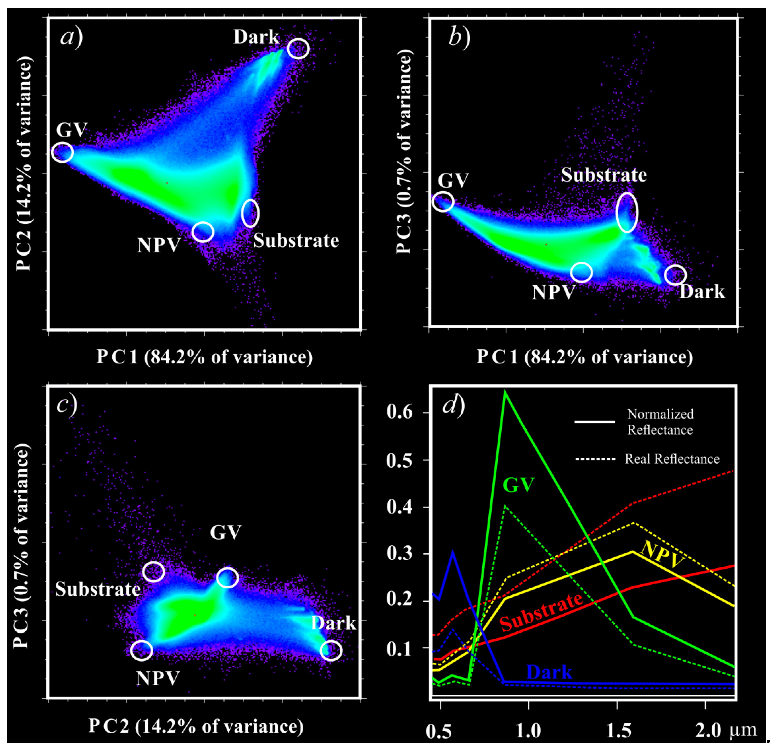
2.3.3. Selection of Endmembers

Endmembers were selected by means of an interactive process based on principal-components analysis (PCA). The rationale of PCA (or Karhune–Loeve analysis) is to eliminate correlation encountered among the original spectral bands, first identifying the axes of greater variance of the data set (in order from the highest to lowest variance) and then rotating those axes orthogonally to a new coordinate system. Considering the present application, PCA makes it possible to reduce the dimensionality of the original dataset by concentrating the greatest proportion of variance into the first principal components [49]. Hence, projecting the first three principal components (PC1, PC2 and PC3) onto a series of two-dimensional (2D) scatterplots makes it possible to visualize the spectral-mixing space (SMS) under analysis.

The SMS can be considered a coordinate space, whereby a pixel at any point location in that space can be described as a mixture of spectral endmembers [37]. Thus, while pure spectra (endmembers) lie at the corners of the SMS, mixed spectra are found within the convex hull or along the straight edges between pairs of endmembers. As can be seen in Figure 2a–c, the combination of PC1 with PC2 covers most of the total variance (~98%), forming a well-defined triangular SMS bounded by the apexes Dark, Green Vegetation (GV), and Substrate/Non-Photosynthetic Vegetation (NPV) spectra endmembers. Combinations of PC1 with PC3 and PC2 with PC3 (accounting for ~85% and ~15% of the total variance, respectively) complement the endmembers selection by distinguishing more clearly between NPV and Substrate spectra, allocating them to diametric apexes.

The four spectra highlighted in Figure 2d correspond to Dark, GV, Substrate and NPV endmembers used in the unmixing modeling. These endmembers represent spectra that are representative of the composition of the mixture of the landscape analyzed and were selected in the following places: in a clean-water area, on an industrial roof and over a large area of green and dry pasture, respectively. During the selection process, we avoided selecting spectra located on the edges of classes to diminish contamination of adjacent radiance; hence, all spectra considered were measured within homogeneous classes. High-resolution Google Earth images were used to aid the identification of the corresponding classes.

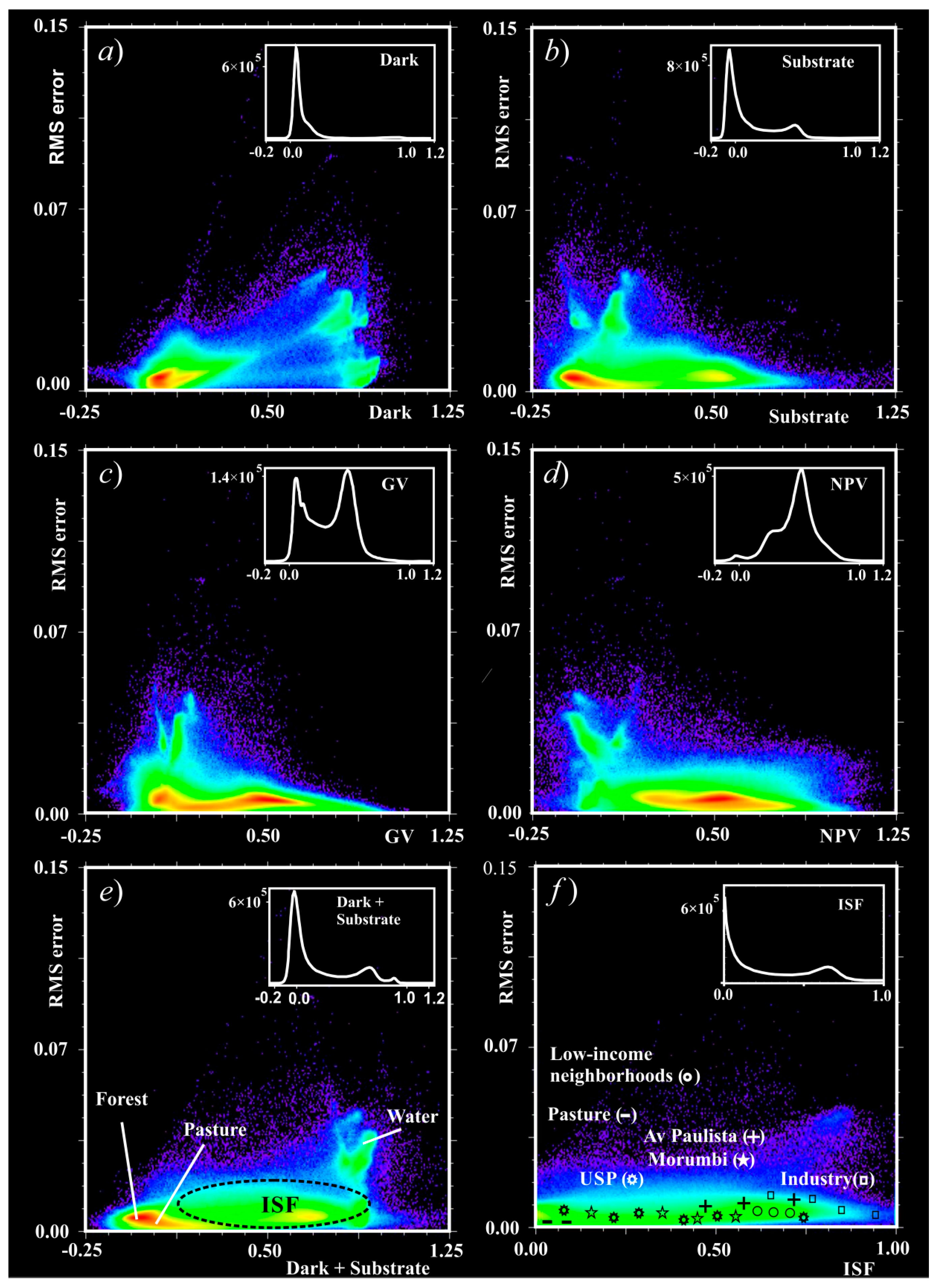
2.3.4. Modeling and Validation of Impervious Surface Fraction (ISF)

ISA is composed of a variety of construction materials with a broad range of energy reflections. In this study, the impervious surface fraction (ISF) was estimated by adding together dark and substrate fraction images derived from the LSMM [14,40] (Figure 1). With this, ISA composed of dark and bright materials, such as asphalt and concrete, appeared in the IFS model with the highest values. Otherwise, non-impervious areas, such as forest lands and green pasture, were modeled with the lowest ISF values.

It is important to note that rivers and lakes in the dark fraction image are modeled with high fractional values similar to those for dark impervious areas. Aiming to circumvent this confusion error, a water mask was created through a classification routine [50] and the ISF values corresponding to rivers and lakes were then assigned to zero. Finally, all pixels with a fraction overflow (with negative values or greater than 1) in the ISF model were constrained to the range 0–1 by applying a practical solution: setting the negative values to zero and those greater than 1 to 1. The rationale for this truncation is that, from an interpretative perspective, negative fractions mean that none of an endmember is present, while fractions greater than 1 mean that an endmember is the only one present [24].

To validate the results, reference ISAs calculated from high-resolution aerial orthophotographs were compared to the ISF estimates generated by the LSMM. A total of 50 samples, following a stratified random sampling scheme, were collected so as to represent the variability of imperviousness in the MRSP. This number of samples is commonly used as a reference to obtain a consistent statistical analysis of the results. Thus, 20 samples were collected in the most central portions of the Sao Paulo metro area, 20 samples in the urban fringe and the remaining 10 samples in rural zones. Each sample accurately described the proportion of ISA within a ground reference of 300 × 300 m, a ground reference much larger than the Landsat-8 OLI pixel size (30 m). This change of scale was intended to: (1) mitigate location errors within orthophotos and satellite images since location errors drop with an increase of measurement size [23,51]; (2) evaluate ISF fluctuations due to changes in the spatial resolution of the image. Thus, to put the validation into practice, the original resolution of the ISF model (with 30-m spatial resolution) was rescaled to 300 m pixel size through an aggregation factor of 10 × 10 pixels, and the resulting pixel values were recalculated as an average function of the finer resolution model.

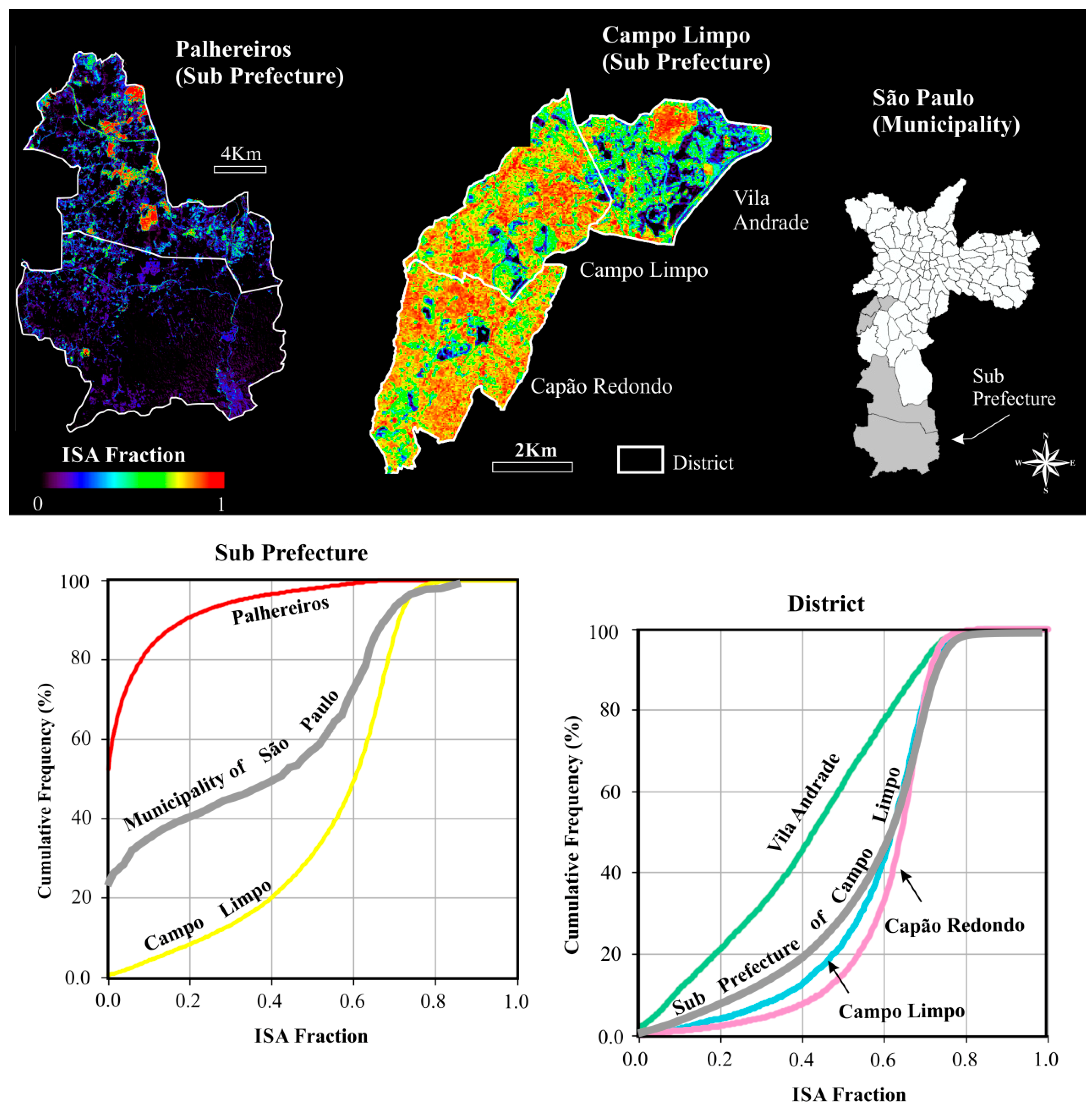
2.4. ISF Model Integration

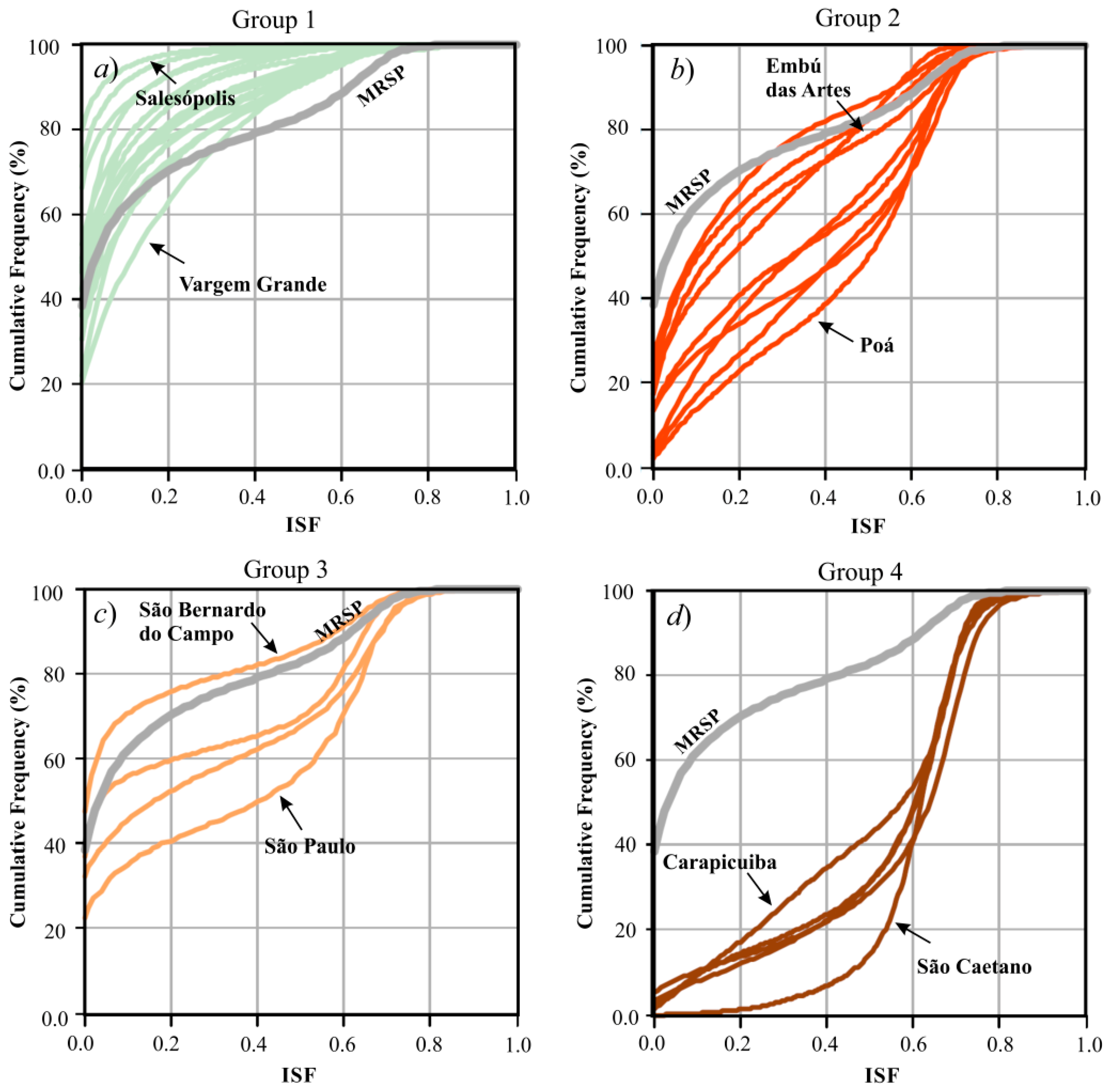
Our approach integrates ISF information into a graph that describes the extent to which the impervious level is concentrated or uniformly dispersed across a set of geographic units. This graph is similar to the Lorenz curve commonly employed to assess the relative income distribution of a population, differing in that the focus is on the distribution of imperviousness. The abscissa shows the ISF values and the ordinate their respective cumulative percentages. This graph is constructed using a simple tabulation procedure. The first step is to order ISF from the lowest to the highest values. The absolute frequency for each ISF value is then transformed into a percentage and, finally, each of these percentages is added up to produce the cumulative numbers needed to plot the curves on the graph [52].

3. Results

On comparing the original reflectance with the normalized reflectance, an amplification of the spectral contrast of the main land-use and land-cover (LULC) types presented in the study area was observed. When uncorrelated PC imagery derived from the normalized imagery was projected onto a series of scatterplots, pure spectra clustered more clearly at corners of distribution (Figure 2a–c), than when using real reflectance images; thus, the process of endmembers selection was made easier and less subjective. This result is explained by the fact that the normalization technique reduces intra-class variability of many LULC categories. In practical terms, as can be seen in Figure 2d, the normalization attenuated the brightness values of the high reflectance endmembers (NPV and Substrate); on the other hand, the normalization scaled up the signature values of moderate/low reflectance endmembers (GV and Dark) along the spectrum. Further details of the normalization effect on the imagery variance can be seen in Wu [23].

The results obtained here also revealed a good accommodation of the spectral endmembers selected in the unmixing process. The RMS error was consistently low (mean = 0.005) and, generally, the fraction estimates are in accordance with the physical structures of the landscape (Figure 3a–d). While fraction-overflow errors were close to zero for Dark, GV and NPV (<1% of the image), for the Substrate fraction, the frequency of pixels modeled with negative values (but close to zero) were considerably higher (~50% of the image). Despite this, the overflow error had little practical effect on the purpose of this research, being circumvented with the simple “truncation” of the data, since such errors are concentrated mainly in the rural areas covered by green vegetation.

After applying the water mask and performing the correction of the fraction-overflow fluctuation, water bodies and rural areas covered by forest, green pasture and agriculture had their pixel values assigned to zero in the final ISF estimate. Additionally, intra-urban variations had their features modeled with a continuous field of values varying according to the size and density of buildings, spatial arrangements of the features and presence of vegetation. The highest ISF rates were found in the LULC classes for industry, commercial/financial centers (such as Avenida Paulista [+]), and high-density, low-income neighborhoods. Meanwhile, the lowest IFSs were in parks, in the University of São Paulo (USP) campus and in wealthy neighborhoods with tree-lined streets (such as Morumbi [⋆]).

When comparing the ISF estimates with reference data from aerial photography, we found that the model adopted predicted ISA considerably well at the 300 × 300-m pixel scale. Figure 4 shows a good linear fit (R² = 0.97) between the reference samples and the estimated ISF rates; the samples clustered along the regression line indicate that the mathematical model is robust for describing imperviousness response. It should be noted that the estimated values were generally lower than expected, especially in areas with larger amounts of ISF. As a consequence, the average value of the generated residuals (Residual = Reference – Estimated) was equal to 7.88, an underestimation error of ~8% on average in the final result.

Figure 5 shows the cumulative ISF curves for the 39 municipalities comprised by the MRSP. The four patterns exhibited in graphs a–d were grouped visually by analyzing the similarity of the curve describing each municipality. Despite the differences seen in amplitudes, the forms of the curves were considered the most important element for grouping the municipalities, because it reveals a pattern underlying the impervious surface distribution that mirrors the spatial organization and functionalities of each municipality within the context of the metro region. Thus, in the following graphs: (a) Group 1 consists of essentially rural municipalities where the economy is focused on agriculture and maintenance of forests and water resource preservation; (b) Group 2 includes municipalities, mainly on the urban fringe, that are either significantly rural or high-density urbanized areas; (c) Group 3 includes municipalities with the second largest rural proportion, but which differs from the previous group due to their greater economic centrality (this group includes the city of São Paulo) and greater similarities with the MRSP in terms of ISF distribution; (d) Group 4 comprises municipalities with higher ISF rates in the metro region.

4. Discussion

An ISF map is an intrinsically physical model of anthropogenic activities in the environment and should not be confused with a “standard” LULC map. This is because a given land class comprises a variety of covers that drive soil imperviousness depending on their composition and functionality. Accordingly, it is very common to find distinct ISF rates distributed over a relatively small area in the urban plot. Residential areas of a high economic standard, for example, tend to have a wide spectrum of land cover, interspersing buildings, street gardens, lawns, etc., resulting in a great fluctuation of ISF. In contrast, densely populated low-income zones have much less variability of cover, resulting in lower fluctuations of ISF.

Indeed, one of the major challenges of mapping ISA through remote sensing is to deal with the great spectral diversity of materials in the built environment. According to Adams and Gillespie [24], there is an implicit assumption in the standard SMA that the spectral properties of endmembers do not vary; only their fractions do. However, in reality, endmember properties vary naturally as a result of intra-class spectral variabilities, thus having a direct impact on the quantification of impervious surfaces [42]. Due to this, procedures that incorporate such variability into the mixture modeling [34,53], or that attenuate their fluctuation values in a preliminary step, have gained importance for the improvement of estimates. The image-normalization technique employed in this study proved to be efficient for this purpose and also provided another advantage: it attenuated the shadowing effects caused by the relief and arrangement of buildings. The normalization technique, however, was not able to circumvent the well-known problem of confusion errors involving high-albedo impervious surface and bright bare soil. Despite this, such errors have little impact on the quality of the final results, given that they occurred locally, over small areas, and clustering along the urban fringe.

For the ISF estimate, the spectral references formed by the Dark, Bright, GV and NPV set were found to be suitable for characterizing the mixture endmembers for the MRSP. Instead of four endmembers, some studies described in the literature suggest using the Dark, Bright and GV triplet to decouple the mixture composition of the urban landscape [37,54]. Small [37], for instance, found in a global analysis that >98 % of the Landsat-7 ETM+ image-spectra variance can be represented in a three-dimensional spectral mixing space. We also tried generating a model using three endmembers (Dark, Bright and GV), but because of the significant presence of dry pasture (the imagery used was taken during the local dry season), a proportion of the area ended up being modeled with a high fraction of Bright endmember, which overestimated the ISF values. It is very likely that, if imagery taken from the rainy season were employed, the aforementioned problem would at least be minimized, since the pasture areas would be dominantly described no longer as a combination including the Bright endmember, but as a modulation of the GV endmember. In some cases, a specific endmember of impervious area has been inserted into the modeling to map ISA [36,55]; however, most of the time, impervious areas (including dark and bright materials), soils and water are problematic to separate.

In principle, interpreting endmember fractions does not depend on the spatial configuration of the image. What really matters are the mixture values encountered in the pixel and the precision level required in the delineation of geometric features. This multi-scale characteristic allows imagery originating from different instruments and with distinct spatial resolutions to be used complementarily, expanding the possibility of monitoring and analysis. The only basic prerequisite for this integration is that the endmember set be previously calibrated with the images used. Another advantage of mixture analysis is that the fraction estimates can be generated either using ad-hoc endmembers to meet site-specific requirements or using generic endmembers obtained from own images or laboratories, making it possible, for instance, to compare fraction endmembers between different cities worldwide.

The Lorenz curve proved to be an effective instrument for describing ISF variation, assisting in the characterization and grouping of municipalities according to the form of the cumulative curves. Another advantage is that the cumulative curve allows direct comparison and analysis between distinct territorial units. Figure 6 highlights the cumulative ISF curves, taking into account the municipality, sub-prefecture and district levels. As can be seen, while the Palhereiros sub-prefecture is mostly rural, the Campo Limpo sub-prefecture is the opposite. However, Campo Limpo is not homogeneous, having a more regular pattern in the districts of Campo Limpo and Capão Redondo (with high population density and low income) and greater internal divergence in the district of Vila Andrade (wealthier and with greater ISF variation due to the greater presence of green streets and garden spaces).

A detailed analysis of ISF variation is useful in a variety of applications. As already mentioned, an increase in constructed impervious surface strongly affects runoff, thus, an adequate measurement of ISF is a prerequisite for strategies aiming to attenuate damage due to episodes of flooding in urban areas. For studies related to urban morphology characterization, it is interesting to consider in the analysis the complementary information derived from LSMM (ISF + GV + Dark) in order to obtain a more comprehensive biophysical characterization of the built environment. This complementary analysis is analogous to the conceptual vegetation–impervious-surface–soil (V–I–S) model proposed by Ridd [56], but with the advantage of including the Dark spectrum in the mixing composition. Dark imagery is useful for urban characterization, because it adds land-cover information related to water/wetland not explained by the V–I–S model [15]. Another interesting possibility is to insert temperature information into the analysis. Dark ISA is confused with water in spectral signatures; however, their land-surface temperatures vary [57], so expert rules could be established to distinguish them automatically with no need for a mask.

Contrasting the cumulative ISF curves from the original 30-m against the resampled 300-m pixel-size model reveals a good accommodation of the data for different territorial units (Figure 7). Four relevant aspects were noted when analyzing the cumulative curves. First, an underestimation error of the ISF model was observed, so all curves reached 100% in the cumulative frequency at values of ISF near 0.7–0.8. Second, the differences between the curves suggest some form of systematic behavior in which the depletion of pixel resolution tends to underestimate the lower fractions and overestimate the higher ones. Third, the highest discrepancy observed in the district of Vila Andrade likely resulted from the zoom-in on the scale of analysis. Finally, the general behavior of the curves also suggests that imperviousness estimates generated from satellite imagery with coarser spatial resolution can be complementarily used to analyze the ISF distribution with a minimum loss in the quality of the final results.

ISA distribution is a function of the population, the availability of surfaces suitable for building and the level of economic development. According to [11], high levels of ISA per capita calculated at nationally aggregated levels generally identify wealthy countries (e.g., high per-capita GDP). Although there may be some degree of correlation, we found no conspicuous relationship between the ISF values on the municipality scale and GDP. Apart from Biritiba Mirim, where the economy is heavily dependent on primary activities (60% of the GDP), the largest share of the economy in all other municipalities is in the secondary and tertiary sectors. As can be seen in Figure 8, the primary sector contributes to less than 5% of the economy for most municipalities, whereas the secondary and tertiary sectors contribute values varying in the ranges of ~5–50% and ~50–95%, respectively. Even considering Group 1, which has the lowest imperviousness rates, the economy related to the primary sector is still of little prominence for the GDP, with values slightly greater than those observed in Groups 2, 3 and 4. These results therefore revealed that, in the context of the MRSP, economic performance related to the primary, secondary and tertiary sectors has little potential for explaining the distribution of impervious areas on the municipality scale. In contrast, we believe that GDP may be used for more generic applications with reasonable success to describe modulation concerning the impervious area. In order to know exactly what these generic applications would be, further studies may be done relating ISA and GDP, shifting the analysis up to the national level.

In recent years, a number of indices have been proposed for describing variations in impervious surface. Here, to make a parallel with the sensitivity of the ISF model, we selected two of the most well-known indices used for mapping ISA: the Normalized Difference Built-up Index (NDBI) [58] and the Normalized Difference Vegetation Index (NDVI) [59]. The NDBI is calculated using the NIR and SWIR-1 channels, and the results range from −1 to 1. The higher the positive NDBI values, the greater the signal contribution for the built areas. The NDVI, on the other hand, is calculated using the Red and NIR channels, with values also ranging from −1 to 1. For ISA applications, NDVI has been used to explore the inverse relationship between the increase in NDVI values and built-up areas [60]. Taking as an example a subset of the study area (Figure 9), contrasting the NDBI (b) and NDVI (c) values against the ISF model revealed a more prominent sensitivity with the model generated in this study. This can be seen more clearly in the scatterplots; while the ISF values keep rising after 0.5, the NDVI values remain practically unchanged after that value. The same can be observed with NDVI, but inversely, reaching a stationary moment near zero. For both the NDBI and the NDVI, the saturations highlighted the superiority of the ISF model for registering the continuous response of soil imperviousness in the urban area.

Finally, ISA is the most remarkable footprint of anthropogenic activities on the environment. A step closer to achieving a better understanding of the impact caused by the advance of anthropogenic surface in the physical and biological environment is to describe its occurrence precisely in terms of areal extent and distribution pattern. Comparing the ISF with distinct territorial units is an excellent asset for sharpening our perception of how the phenomenon is imbricated in geographical space. Furthermore, approaches highlighting a multi-scalar dimension in their analyses have great opportunities for providing knowledge of patterns and processes still little explored in the scientific literature.

5. Conclusions

One of the biggest challenges of mapping ISA through moderated spatial-resolution optical images is coping with the high spectral diversity and mixture components registered at the pixel scale. ISAs feature a complex spectral behavior, ranging from low albedo to high albedo. The spectral-mixture analysis constitutes an excellent asset for circumventing the difficulties in mapping impervious surfaces in urban areas, so it entails a physical basis of either intra-spectral variability or the pixel-mixing effect. Four endmembers—Dark, Substrate, Green Vegetation (GV) and Non-Photosynthetic Vegetation (NPV)—proved to be efficient in revealing the spectral variability of the study site. Summing the Dark and Substrate fraction components derived from the mixture analysis accurately reflected the impervious surface fraction (ISF) abundance, and the results made it possible to quantify areal extent as well as to analyze impervious areas across different scale units. Comparing the original 30-m ISF model with an aggregated 300-m ISF model, the cumulative curves highlighted a good match in their distribution, suggesting that imagery with different spatial configurations can be used in a complementary and robust way to study impervious areas. Ultimately, the ISF model was found to be more sensitive in describing impervious surface response than other well-known indices, such as NDVI and NDBI.

References

1. Tocci, C.E.M. Água no meio urbano. In Águas Doces No Brasil: Capital Ecológico, Uso e Conservação; Rebouças, A.C., Braga, B., Tundisi, J.G., Eds.; Escrituras: São Paulo, Brasil, 2002; pp. 473–502. [Google Scholar]
2. Pappas, E.A.; Smith, D.R.; Huang, C.; Shuster, W.D.; Bonta, J.V. Impervious surface impacts to runoff and sediment discharge under laboratory rainfall simulation. Catena 2008, 72, 146–152. [Google Scholar] [CrossRef]
3. Chormanski, J.; Van de Voorde, T.; De Roeck, T.; Batelaan, O.; Canters, F. Improving distributed runoff prediction in urbanized catchments with remote sensing based estimates of impervious surface cover. Sensors 2008, 8, 910–932. [Google Scholar] [CrossRef]
4. Changnon, S.A. Inadvertent weather modification in urban areas: Lessons for global climate change. Bull. Am. Meteorol. Soc. 1992, 73, 619–627. [Google Scholar] [CrossRef]
5. Yuan, F.; Bauer, M.E. Comparison of impervious surface area and normalized difference vegetation index as indicators of surface urban heat island effects in Landsat imagery. Remote Sens. Environ. 2007, 106, 375–386. [Google Scholar] [CrossRef]
6. Xu, H.; Lin, D.; Tang, F. The impact of impervious surface development on land surface temperature in a subtropical city: Xiamen, China. Int. J. Climatol. 2012, 33, 1873–1883. [Google Scholar] [CrossRef] [Green Version]
7. Liu, K.; Fang, J.; Zhao, D.; Liu, X.; Zhang, X.; Wang, X.; Li, X. An assessment of urban surface energy fluxes using a sub-pixel remote sensing analysis: A case study in Suzhou, China. ISPRS Int. J. Geo-Inf. 2016, 5, 11. [Google Scholar] [CrossRef]
8. Schueler, T.R. The Importance of imperviousness. Waters Prot. Tech. 1994, 1, 100–111. [Google Scholar]
9. Arnold, C.L.; Gibbons, C.J. Impervious surface coverage: The emergence of a key environmental indicator. J. Am. Plan. Assoc. 1996, 62, 243–258. [Google Scholar]
10. White, M.D.; Greer, K.A. The effects of watershed urbanization on the stream hydrology and riparian vegetation of Los Pe˜nasquitos Creek, California. Landsc. Urban Plan. 2006, 74, 125–138. [Google Scholar] [CrossRef]
11. Elvidge, C.D.; Tuttle, B.T.; Sutton, P.C.; Baugh, K.E.; Howard, A.T.; Milesi, C.; Bhaduri, B.L.; Nemani, R. Global distribution and density of constructed impervious surfaces. Sensors 2007, 7, 1962–1979. [Google Scholar] [CrossRef] [PubMed]
12. Guo, W.; Lu, D.; Wu, Y.; Zhang, J. Mapping impervious surface distribution with integration of SNNP VIIRS-DNB and MODIS NDVI data. Remote Sens. 2015, 7, 12459–12477. [Google Scholar] [CrossRef]
13. Slonecker, E.T.; Jennings, D.B.; Garofalo, D. Remote sensing of impervious surfaces: A review. Remote Sens. Rev. 2001, 20, 227–255. [Google Scholar] [CrossRef]
14. Weng, Q. Remote sensing of impervious surfaces in the urban areas: Requirements, methods, and trends. Remote Sens. Environ. 2012, 117, 34–49. [Google Scholar]
15. Lu, D.; Li, G.; Kuang, W.; Moran, E. Methods to extract impervious surface areas from satellite images. Int. J. Digit. Earth 2014, 7, 93–112. [Google Scholar]
16. Small, C. A global analysis of urban reflectance. Int. J. Remote Sens. 2005, 26, 661–681. [Google Scholar] [CrossRef]
17. Herold, M.; Roberts, D.A. The spectral dimension in urban remote sensing. In Remote Sensing of Urban and Suburban Areas; Rashed, T., Jürgens, C., Eds.; Springer: Austin, TX, USA, 2010; pp. 47–65. [Google Scholar]
18. Lu, D.; Hetrick, S.; Moran, E. Impervious surface mapping with Quickbird imagery. Int. J. Remote Sens. 2011, 32, 2519–2533. [Google Scholar] [CrossRef] [PubMed] [Green Version]
19. Yang, L.; Huang, C.; Homer, C.G.; Wylie, B.K.; Coan, M.J. An approach for mapping large-area impervious surfaces: Synergistic use Landsat-7 ETM+ and high spatial resolution imagery. Can. J. Remote Sens. 2003, 29, 230–240. [Google Scholar]
20. Lu, D.; Li, G.; Moran, E.; Batistella, M.; Freita, C.C. Mapping impervious surfaces with the integrated use of Landsat Thematic Mapper and radar data: A case study in an urban–rural landscape in the Brazilian Amazon. ISPRS J. Photogramm. Remote Sens. 2011, 66, 798–808. [Google Scholar] [CrossRef] [Green Version]
21. Parece, T.E.; Campbell, J.B. Comparing urban impervious surface identification using landsat and high resolution aerial photography. Remote Sens. 2013, 5, 4942–4960. [Google Scholar]
22. Small, C. High spatial resolution spectral mixture analysis of urban reflectance. Remote Sens. Environ. 2003, 88, 170–186. [Google Scholar]
23. Wu, C. Quantifying high-resolution impervious surfaces using spectral mixture analysis. Int. J. Remote Sens. 2009, 30, 2915–2932. [Google Scholar] [CrossRef]
24. Adams, J.B.; Gillespie, A.R. Remote Sensing of Landscape with Spectral Images: A Physical Modelling Approach; Cambridge University Press: New York, NY, USA, 2006. [Google Scholar]
25. Kawakubo, F.S.; Morato, R.G.; Luchiari, A. Use of fraction imagery, segmentation and masking techniques to classify land-use and land-cover types in the Brazilian Amazon. Int. J. Remote Sens. 2013, 34, 5452–5467. [Google Scholar] [CrossRef]
26. Adams, J.B.; Smith, M.O.; Johnson, P.E. Spectral mixture modeling: A new analysis of rock and soil types at the Viking Lander 1 site. J. Geophys. Res. 1986, 91, 8098–8112. [Google Scholar] [CrossRef]
27. Drake, N.A.; Mackin, S.; Settle, J.J. Mapping vegetation, soils, and geology in semiarid shrublands using spectral matching and mixture modeling of SWIR AVIRIS imagery. Remote Sens. Environ. 1999, 68, 12–25. [Google Scholar] [CrossRef]
28. Shimabukuro, Y.E.; Batista, G.T.; Mello, E.M.K.; Moreira, J.C.; Duarte, V. Using shade fraction image segmentation to evaluate deforestation in Landsat Thematic Mapper images of the Amazon region. Int. J. Remote Sens. 1998, 19, 535–541. [Google Scholar] [CrossRef]
29. Souza, C., Jr.; Firestone, L.; Silva, L.M.; Roberts, D.A. Mapping forest degradation in the Eastern Amazon from Spot 4 through spectral mixture models. Remote Sens. Environ. 2003, 87, 494–506. [Google Scholar] [CrossRef]
30. Anderson, L.O.; Shimabukuro, Y.E.; Defries, R.S.; Morton, D. Assessment of deforestation in near real time over the Brazilian Amazon using multitemporal fraction images derived from Terra MODIS. IEEE Geosci. Remote Sens. Lett. 2005, 2, 315–318. [Google Scholar] [CrossRef]
31. Cochrane, M.A.; Souza, C.M., Jr. Linear mixture model classification of burned forests in the Eastern Amazon. Int. J. Remote Sens. 1998, 19, 3433–3440. [Google Scholar] [CrossRef]
32. Quintano, C.; Fernández-Manso, A.; Roberts, D.A. Multiple endmember spectral mixture analysis (MESMA) to map burn severity levels from Landsat images in Mediterranean countries. Remote Sens. Environ. 2013, 136, 76–88. [Google Scholar] [CrossRef]
33. Roberts, D.A.; Smith, M.O.; Adams, J.B. Green vegetation, non-photosynthetic vegetation and soils in AVIRIS data. Remote Sens. Environ. 1993, 44, 255–269. [Google Scholar] [CrossRef]
34. Roberts, D.A.; Gardner, M.; Church, R.; Ustin, S.; Scheer, G.; Green, R.O. Mapping chaparral in the Santa Monica Mountains using multiple endmember spectral mixture models. Remote Sens. Environ. 1998, 65, 267–279. [Google Scholar] [CrossRef]
35. Kawakubo, F.S.; Pérez Machado, R.P. Mapping coffee crops in southeastern Brazil using spectral mixture analysis and data mining classification. Int. J. Remote Sens. 2016, 37, 3414–3436. [Google Scholar] [CrossRef]
36. Rashed, T.; Weeks, J.R.; Roberts, D.; Rogan, J.; Powell, R. Measuring the physical composition of urban morphology using multiple endmember spectral mixture models. Photogramm. Eng. Remote Sens. 2003, 69, 1011–1020. [Google Scholar] [CrossRef]
37. Small, C. The Landsat ETM+ spectral mixing space. Remote Sens. Environ. 2004, 93, 1–17. [Google Scholar] [CrossRef]
38. Small, C.; Lu, J.W.T. Estimation and vicarious validation of urban vegetation abundance by spectral mixture analysis. Remote Sens. Environ. 2006, 100, 441–456. [Google Scholar] [CrossRef]
39. Pérez Machado, R.P.; Small, C. Identifying multi-decadal changes of the Sao Paulo urban agglomeration with mixed remote sensing techniques: Spectral mixture analysis and night-lights. Earsel Eproc. 2013, 12, 101–112. [Google Scholar]
40. Wu, C.; Murray, A.T. Estimating impervious surface distribution by spectral mixture analysis. Remote Sens. Environ. 2003, 84, 493–505. [Google Scholar] [CrossRef]
41. Yang, F.; Matsushita, B.; Fukushima, T. A pre-screened and normalized multiple endmember spectral mixture analysis for mapping impervious surface area in Lake Kasumigaura Basin, Japan. ISPRS J. Photogramm. Remote. Sens. 2010, 65, 479–490. [Google Scholar] [CrossRef] [Green Version]
42. Jacobson, C.R. The effects of endmember selection on modelling impervious surfaces using spectral mixture analysis: A case study in Sydney, Australia. Int. J. Remote Sens. 2014, 35, 715–737. [Google Scholar] [CrossRef]
43. Li, L.; Lu, D.; Kuang, W. Examining urban impervious surface distribution and its dynamic change in Hangzhou metropolis. Remote Sens. 2016, 8, 265. [Google Scholar] [CrossRef]
44. Emplasa. Available online: https://www.emplasa.sp.gov.br/ (accessed on 10 May 2018).
45. Harris. Available online: https://www.harrisgeospatial.com/ (accessed on 10 February 2018).
46. Wu, C. Normalized spectral mixture analysis for monitoring urban composition using ETM+ imagery. Remote Sens. Environ. 2004, 93, 480–492. [Google Scholar] [CrossRef]
47. Zhang, J.; Benoit, R.; Arturo, S. Spectral unmixing of normalized reflectance data for the deconvolution of lichen and rock mixtures. Remote Sens. Environ. 2005, 95, 57–66. [Google Scholar] [CrossRef]
48. Van de Voorde, T.; De Roeck, T.; Canters, F. A comparison of two spectral mixture modelling approaches for impervious surface mapping in urban areas. Int. J. Remote Sens. 2009, 30, 4785–4806. [Google Scholar] [CrossRef]
49. Jensen, J. Introductory. In Digital Image Processing: A Remote Sensing Perspective, 3rd ed.; Prentice Hall: Upper Saddle River, NJ, USA, 2005. [Google Scholar]
50. Sohn, Y.; Rebello, N.S. Supervised and unsupervised spectral angle classifiers. Photogramm. Eng. Remote Sens. 2002, 68, 1271–1280. [Google Scholar]
51. Pontius, R.G., Jr. Quantification error versus location error in comparison of categorical maps. Photogramm. Eng. Remote Sens. 2000, 66, 1011–1016. [Google Scholar]
52. Plane, D.A.; Rogerson, P.A. The Geographical Analysis of Population with Applications to Planning and Business; John Wiley & Sons: New York, NY, USA, 1994. [Google Scholar]
53. Asner, G.P.; Lobell, D.B. A biogeophysical approach for automated SWIR unmixing of soils and vegetation. Remote Sens. Environ. 2000, 74, 99–112. [Google Scholar] [CrossRef]
54. Small, C. Comparative analysis of urban reflectance and surface temperature. Remote Sens. Environ. 2006, 104, 168–189. [Google Scholar] [CrossRef]
55. Phinn, S.; Stanford, M.; Scarth, P.; Murray, A.T.; Shyy, P.T. Monitoring the composition of urban environments based on the Vegetation-Impervious Surface-Soil (VIS) model by subpixel analysis techniques. Int. J. Remote Sens. 2002, 23, 4131–4153. [Google Scholar] [CrossRef]
56. Ridd, M.K. Exploring a V-I-S (Vegetation-Impervious Surface-Soil) model for urban ecosystem analysis through remote sensing: Comparative anatomy for cities. Int. J. Remote Sens. 1995, 16, 2165–2185. [Google Scholar] [CrossRef]
57. Lu, D.; Weng, Q. Use of impervious surface in urban land use classification. Remote Sens. Environ. 2006, 102, 146–160. [Google Scholar] [CrossRef]
58. Zha, Y.; Gao, J.; Ni, S. Use of normalized difference built-up index in automatically mapping urban areas from TM imagery. Int. J. Remote Sens. 2003, 24, 583–659. [Google Scholar] [CrossRef]
59. Rouse, J.W.; Haas, R.H.; Schell, J.R.; Deering, D.W. Monitoring vegetation systems in the Great Plains with ETRS. In Third Earth Resources Technology Satellite-1 Symposium-Volume I: Technical Presentations; NASA SP-351; NASA: Washington, DC, USA, 1974; p. 309. [Google Scholar]
60. Martins, M.H.; Morato, R.G.; Kawakubo, F.S. Mapping impervious surface areas using orthophotos, satellite imagery and linear regression. RDG 2018, 35, 91–101. [Google Scholar]
Figure 1. The Metropolitan Region of São Paulo (MRSP) and the spatial configuration of impervious surface (ISF) values. The areas with lower imperviousness rates (<20%) are rural zones dedicated to agriculture and protection of forest and water sources. The estimate of ISF was generated using Landsat-8 Operational Land Imager (OLI) imagery acquired on 23 August 2015. The spatial resolution of the image is 30 m.
Remotesensing 11 00944 g001
Figure 2. Location of the four endmembers, Dark, GV, Substrate and NPV in a series of two-dimensional (2D) scatterplots (ac). The first three principal components (PCs) account for >99% of variance, with information concentrated primarily in PC1 (84.2%) and PC2 (14.2%). Endmember spectra, real and normalized reflectance (depicted by dashed and continuous lines, respectively), are shown in (d).
Remotesensing 11 00944 g002
Figure 3. Relationship between theRMS)error and the fractional values for Dark (a), Substrate (b), GV (c), NPV (d), Dark + Substrate (e), and ISF model (f). Note: In the color scale, pixel density rises from cold to warm colors. Avenida Paulista is the main financial center of the state of São Paulo, with high construction density and low vegetation rates. Morumbi is a wealthy, green neighborhood of the city of São Paulo. The campus of the University of São Paulo (USP) is a large structure interspersed with green vegetation (urban forest and grass).
Remotesensing 11 00944 g003
Figure 4. ISF validation. The reference data set (n = 50) was calculated from aerial orthophotography using a 300 × 300-m grid as a reference (see explanation in text). The dashed line is the 1:1 line and the solid line is the regression line.
Remotesensing 11 00944 g004
Figure 5. Grouping of the relative distributions of ISF in the MRSP. The municipalities highlighted in the graphs are representative for each group, setting the upper and lower limits. The location of these municipalities is shown in Figure 1.
Remotesensing 11 00944 g005
Figure 6. ISF distributions for different territorial units: municipality, sub-prefecture and district.
Remotesensing 11 00944 g006
Figure 7. Cumulative ISF curves recorded for pixel sizes of 30 m (solid lines) and 300 m (dashed lines).
Remotesensing 11 00944 g007
Figure 8. Contributions of the primary, secondary and tertiary sectors to the gross domestic product (GDP) of the municipalities of the MRSP (according to Emplasa). Groups 1 to 4 were defined according to the cumulative-frequency curves shown in Figure 5.
Remotesensing 11 00944 g008
Figure 9. Subset of the study area: (a) ISF model; (b) NDBI; (c) NDVI index; (d) color composition ISF (R), NDVI (G), NDBI (B). The higher the image values, the brighter the grey tones.
Remotesensing 11 00944 g009