A Controllable Success Fix Rate Threshold Determination Method for GNSS Ambiguity Acceptance Tests


1
State Key Laboratory of Information Engineering in Surveying, Mapping and Remote Sensing, Wuhan University, Wuhan 430079, China
2
Collaborative Innovation Center for Geospatial Technology, Wuhan 430079, China
3
School of Geodesy and Geomatics, Wuhan University, Wuhan 430079, China
4
School of Electronic and Information Engineering, Beihang University, 37 Xueyuan Road, Beijing 100083, China
5
School of Electrical Engineer and Computer Science, Queensland University of Technology, Brisbane QLD 4001, Australia
*
Author to whom correspondence should be addressed.
Remote Sens. 2019, 11(7), 804; https://doi.org/10.3390/rs11070804
Submission received: 27 February 2019
/
Revised: 30 March 2019
/
Accepted: 1 April 2019
/
Published: 3 April 2019
(This article belongs to the Special Issue High-precision GNSS: Methods, Open Problems and Geoscience Applications)
Abstract
:Global navigation satellite system (GNSS) integer ambiguity acceptance test is one of the open problems in GNSS data processing. A number of ambiguity acceptance tests have been proposed from different perspectives and then unified into the integer aperture estimation framework. The existing comparative studies indicate that the impact of test statistics form on the test performance is less critical, while how to construct an efficient, practical test threshold is still challenging. Based on the likelihood ratio test theory, a new computationally efficient ambiguity acceptance test with controllable success fix rate, namely the fixed likelihood ratio (FL-) approach is proposed, which does not require Monte Carlo simulation. The study indicates that the fixed failure rate (FF-) approach can only control the overall failure rate of the acceptance region, but the local failure rate is not controllable. The proposed FL-approach only accepts the fixed solution meeting the likelihood ratio requirement. With properly chosen likelihood ratio threshold, the FL-approach achieves comparable success rate as the FF-approach and even lower failure rate than the FF-approach for the strong underlying model cases. The fixed success fix rate of the FL-approach is verified with both simulation data and real GNSS data. The numerical results indicate that the success fix rate of the FL-approach achieves >98% while the failure rate is <1.5%. The real-time kinematic (RTK) positioning with ambiguities tested by the FL-approach achieved 1–2cm horizontal precision and 2–4 cm vertical precision for all tested baselines, which confirms that the FL-approach can serve as a reliable and efficient threshold determination method for the GNSS ambiguity acceptance test problem.
1. Introduction
Global navigation satellite system (GNSS) integer ambiguity resolution is the key issue for carrier phase-based fast precise positioning, while the ambiguity acceptance test problem is considered as one of the remaining open problems in GNSS data processing [1]. The mathematical model for the carrier phase-based GNSS positioning model can be expressed as:
where and are the integer and real-valued parameters respectively. The real-valued parameters can be the position, the tropospheric delay, the ionospheric delay and possibly hardware biases. The integer parameters normally refer to the undifferenced or double-differenced carrier phase integer ambiguity parameter. and are corresponding design matrices. The observation vector follows -dimensional multivariate normal distribution with its variance-covariance (vc-) matrix . and are the mathematical expectation and variance operator, respectively.
The mixed integer model can be solved by a four-step procedure:
- Estimating and with the standard least-squares or Kalman filter. The integer nature of is not considered and its real-value estimates are treated as ‘float solution’. The real-valued estimates of and , and their variance-covariance matrix are denoted as:
- Mapping the real-valued ambiguity vector to an integer vector with an integer estimator. The integer estimation procedure can be described as , with .
- Validating the fixed integer with the ambiguity acceptance tests. If is rejected by the acceptance test, it means that the fixed integer is not considered as a correct integer solution
- Updating the real-valued parameters by if is accepted by ambiguity acceptance test. If is rejected by the test, the float solution is used as the final solution.
The ambiguity acceptance test can be treated as either a hypothesis test problem or an estimation problem. A standard hypothesis test problem includes three aspects: the probability basis, the test statistic, and the threshold. The ambiguity acceptance test problem can be formulated as:
where is the true ambiguity vector. The ambiguity acceptance test is a composite hypotheses test since the float solution can be mapped to arbitrary integer vectors, while only one of them is correct. Generally, a hypothesis test has four types of potential outcomes, which are outlined in Table 1. The table is often referred to as the decision matrix [2]. In the decision matrix, the false alarm and miss detection cases are unwanted outcomes. The miss detection can cause incorrect ambiguity fix, which introduces unexpected bias in the final positioning results. The hypothesis test theory expressed in the Equation (3) has been well established, but the ambiguity acceptance test is not a standard hypothesis test. The true ambiguity vector is normally unknown in reality, so the ambiguity acceptance test can only use the float solution and the fixed solution for test statistics construction.
Normally, the test statistics of ambiguity acceptance test are constructed based on the ambiguity residual distribution. The ambiguity residual is defined as [3,4]:
The float solution follows the normal distribution, while the fixed solution is not deterministic. As a result, the probability density distribution of ambiguity residuals becomes non-standard. Considering the stochastic property of , the probability density function (PDF) the ambiguity residual is defined as [4]:
where is the pull-in region of integer estimation centered at . is the PDF of float ambiguity . According to the integer aperture (IA) estimation theory, the probability of the ambiguity acceptance test outcomes can be calculated by [5,6]:
where , and are the success rate, the failure rate, and the undecided rate respectively. is the output of integer aperture estimator. and are the acceptance region space and a specific acceptance region centered at . According to the probability foundation and the integer aperture framework, the hypothesis test model for the ambiguity acceptance test model can be illustrated in Figure 1. The area of the red region, the green region, and the grey region corresponds to , and . A detailed description of the ambiguity acceptance test model can be found in [7,8].
A number of test statistics have been constructed to solve the ambiguity acceptance test problem. In early studies, many ambiguity acceptance tests were derived from different perspectives, such as the F-ratio test [9,10], the ratio test [11], the difference test [12], the projector test [13,14], etc. These test statistics are empirically efficient, although some of them are not theoretical rigorous [15]. Within the framework of the integer aperture estimation, the ellipsoidal integer aperture [5], the integer aperture bootstrapping [16], the integer aperture least-squares [17], the penalized integer aperture [18], and the optimal integer aperture [19] have been proposed. An extensive comparison between different integer aperture estimators has been made and the results indicate that the ratio and the difference tests are suboptimal estimators in terms of fixed failure rate [3,20]. The reason for sub-optimality has been analyzed in [21]. The numerical results indicate that the success rate discrepancy between the optimal solution (OIA) and the suboptimal solution is not very significant [3], so the test statistics should not be the key issue in ambiguity acceptance test.
The remaining challenge is how to reasonably determine the threshold of the ambiguity acceptance test. In the early stage, the empirical threshold is adopted. Then, the theoretical rigorous threshold determination method namely the fixed failure rate (FF-) approach is proposed. The FF-approach is considered a promising threshold determination test, but is not computationally efficient enough. In order to overcome this problem, we propose the look-up table method [22,23] and the threshold function method [8,24,25].
The FF-approach can only control the overall failure rate of the acceptance region. To overcome this weakness, a fixed likelihood ratio (FL-) approach is proposed to derive the reliable integer ambiguities by only accepting the integer vector with high likelihood ratio.
2. The Fixed Likelihood Ratio Threshold Determination Approach
In this section, the related work on threshold determination methods in GNSS ambiguity acceptance test is briefly reviewed. The weakness of the FF-approach is then identified accordingly. Next, we proposed the fixed likelihood ratio (FL-) threshold for threshold determination.
2.1. Related Threshold Determination Methods
There are several threshold determination methods related to the ambiguity acceptance test. They can be classified into three types: empirical method, significance test method, and fixed failure rate (FF-) approach [20].
The empirical approach is to determine the threshold according to individual experience. This approach has no sound theoretical basis, but it empirically makes sense. This is a simple and straightforward method, which has been widely used in discrimination tests [9,10,11,12,26,27]. The drawback of the empirical approach is its poor adaptive capacity. One empirical threshold only fits one particular underlying model, a different underlying model and different observation scenario may require different thresholds, which is why the optimal empirical threshold is always controversial.
The significance test approach determines its threshold according to a given significance level α, which corresponds to the false alarm probability (type I error probability) in the decision matrix (Table 1). In the early stage, the ambiguity acceptance test problem is attempted to be solved like the other general hypothesis test problems, and their threshold is often determined with the significance test approach [13,14]. In GNSS ambiguity resolution, the price of making type II errors is far higher than making type I errors. Hence controlling the significance level makes it difficult to achieve a reliable solution, although it is popular in the statistics field.
The fixed failure rate (FF-) approach is considered as a promising method and it comes with a rigorous theoretical basis. It determines the threshold according to failure rate tolerance, so it becomes increasingly popular. The objective function of the FF-approach is given as [19,22,23]:
where is the user-specified failure rate tolerance.
The failure rate corresponds to the Type II error in the decision matrix, so the FF-approach is essentially different from the significance test in that the FF-approach controls the type II error, while the significance test controls type I error. Controlling type II error means controlling the failure acceptance risk, which meets the requirement of reliability control in ambiguity resolution.
The FF-approach is theoretically rigorous, but the challenges come from implementation aspects. Calculating the FF-threshold requires an explicit relationship between the failure rate and threshold . According to the definition of IA estimation, the failure rate can be calculated by integrating PDF over different acceptance regions. The PDF is the underlying model specified, and the acceptance region is determined by the underlying model, IA estimator, and the threshold. For a particular model and IA estimator, there is no explicit relationship between threshold and failure rate tolerance . In order to address the relationship, the Monte-Carlo method is used. A large number of samples is used to approximate the distribution of in multi-dimensional space, then the failure rate is computed by testing the fixed solution of each sample. The Monte-Carlo simulation is computation extensive, so a number of algorithms have been proposed to improve the computation efficiency, such as the look-up table method [22,23], the threshold function method [8,24], etc.
2.2. The Likelihood Ratio Integer Aperture Estimation
We now address problems of the FF-approach before offering a solution. A question about the FF-approach is whether it ensures that the accepted ambiguities are reliable. Recalling Equation (6), the failure rate is the integral of the PDF over the acceptance region, which corresponds to the area of the green region in Figure 1. However, the PDF is not evenly distributed, meaning that the failure risk is not homogeneously distributed in the acceptance region. The FF-approach can only control the overall failure rate of the acceptance region and the distribution of is not considered by the failure rate indicator. Considering the inhomogeneous distribution of , it is possible to find a subset of the acceptance region having , where is the acceptance region of the FF-approach. For convenience, we define the local failure rate as:
where is the local failure rate in the subset . The local failure rate refers to the failure probability if the samples fall in a subset region . In contrast, the FF-approach controls the overall acceptance region, which can be expressed as . In practice, if the overall failure rate is controlled, this does not mean that the local failure rate is controllable.
From this perspective, we propose the fixed likelihood ratio approach to control the local failure risk within the acceptance region. The distribution specified failure risk can be measured by the likelihood ratio. According to the hypothesis model (3), the likelihood function for the ambiguity acceptance test can be expressed as [28]:
The likelihood function is the ratio of the PDF subject to the null and alternative hypotheses. If the ratio is large enough, H0 is considered to be reliable. A corresponding likelihood ratio test can be expressed as:
where is the likelihood ratio threshold. The float solution with likelihood ratio smaller than is considered not being sufficiently reliable and thus being rejected. In this test, the likelihood threshold is fixed, which is denoted as the fixed likelihood ratio (FL-) approach. Based on the FL-approach, a new integer aperture estimator can be constructed, which is denoted as the likelihood ratio integer aperture (LRIA). The corresponding acceptance region can be given as:
where is the normalized likelihood ratio threshold, which varies in the interval [0, 1]. is the ratio of float ambiguity PDF and ambiguity residual PDF, which is denoted as the normalized likelihood ratio (NLR) in this context. Larger means higher reliability.
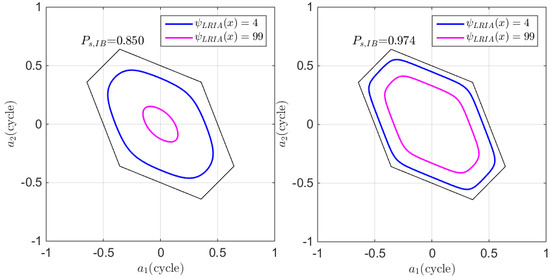
A two-dimensional example of the LRIA acceptance region is illustrated in Figure 2. The figure gives two underlying models with different integer bootstrapping (IB) success rate. The integer bootstrapping success rate is an easy-to-evaluate, tight lower bound of ILS success rate, and often used as the underlying model strength indicator [29], which is denoted as The model with higher IB success rate is considered having a stronger underlying model. The figure indicates that the LRIA acceptance region’s shape depends on the underlying model and threshold. The acceptance region would appear as a hexagon shape for the stronger model and appear as an ellipse shape for the weaker model. Since LRIA and OIA use the same test statistics, the acceptance region’s shape for LRIA was also the same as that for OIA. Therefore, LRIA inherits the optimal acceptance region shape from OIA test statistics.
In the context of underlying principles, a comparison of the FF-approach and FL-approach is demonstrated in Figure 3. In the figure, the red solid line and blue solid lines are the failure rate and normalized likelihood ratio respectively. and are the NLR tolerance and failure rate tolerance, respectively. Two extreme cases, namely a strong underlying model (left panel) and a weak underlying model (right panel) model were examined. In this example, the same threshold = 0.5% and = 0.9 were applied to both examples. For the strong model case, the FF-approach accepts all given by the integer least-squares (ILS) estimator since . However, the figure also indicates that = 0.5. In this example the region < 0.9 will be rejected by the FL-approach since they cannot meet the reliability indicator, while they are accepted by the FF-approach since there is an abundant failure rate budget. Actually, when is fairly close to the ILS pull-in region boundary, it is often unreliable regardless of strong or weak models. The right panel shows the weak underlying model case. In this case, the FF-approach uses up its failure rate budget to earn a small acceptance region since the failure rate rises rapidly. However, the figure also indicates , so the FL-approach gives an empty acceptance region. In fact, the FF-approach will never give an empty acceptance region even in the poor underlying model case, but the reliability will not be guaranteed.
2.3. Properties of LRIA
The likelihood ratio value can reflect the likelihood of the null hypothesis to be true, so it can be used as a threshold of the ambiguity acceptance test. The integer aperture (LRIA) estimation determines the threshold according to the likelihood ratio criterion, which can be equivalently expressed as:
where is the user specified likelihood ratio threshold. The likelihood ratio approach is firstly used to validate the integer bootstrapping estimation with a threshold of 0.99 [30]. The likelihood ratio approach can adjust the acceptance region size automatically according to model strength. The properties of the LRIA are discussed.
2.3.1. The Success Fix Rate Property
The first good property of LRIA is its success fix rate property. According to the definition of LRIA, , so the integration form can be given as:
The detailed proof of Equation (13) is given in Appendix A. The equation indicates can be viewed as a lower bound of success fix rate, so success fix rate can be guaranteed with the likelihood ratio approach. The relationship between and in the one-dimensional case is illustrated in Figure 4. The figure indicates that is always higher than . The discrepancy between and depends on both the underlying model and the threshold itself. is a tight lower bound of the success fix rate in the strong underlying model scenario. When the acceptance region is small, the discrepancy between and is small. However, was reduced to 0.5 at the boundary of the acceptance region, while the decrease of slowed down.
2.3.2. The Local Failure Rate Property
The second property of LRIA is its local failure rate property. According to Equation (12), the local failure rate can be expressed as:
where is the local success rate, . The detailed proof procedure of Equation (14) is given in Appendix B. The equation indicates that the upper bound of the local failure rate is not a constant value for the FL-approach—it is defined by the local success rate. The smaller local success rate also indicates a smaller failure rate upper bound. Although the FL-approach does not have a constant local failure rate, it gives stricter failure rate upper bound in a small local success rate scenario; however, it is still promising for GNSS ambiguity reliability control.
2.3.3. Computational Complexity
The FL-approach employs a user-specified reliability indicator, which does not require Monte-Carlo simulation to determine the threshold, it is therefore more efficient than the FF-approach. The FF-approach requires a Monte-Carlo simulation procedure to address the relationship between the failure rate and the threshold. In contrast, the threshold of the FL-approach can be directly specified according to its success fix rate requirement. It is impossible to compute the exact value of , so an approximation method must be employed. With a fixed numerical error tolerance, the number of integers involved in the computation of depends on the underlying model [31]. A weaker underlying model involves more integers and thus more extensive computation. The relationship between the underlying model’s strength and integer number has been examined in [32]. It can guarantee that the success fix rate is always higher than , but it is only applicable to the IA estimator employing the likelihood ratio test form, such as the LRIA and the difference test integer aperture (DTIA).
2.4. The Relationship between the FL-Threshold and the Model Strength
The underlying model’s strength is the dominant factor for region size acceptance, but different threshold determination methods have different behaviors. For the one-dimensional ambiguity acceptance test, the thresholds given by the FL-approach and FF-approach for the different underlying models are presented in Figure 5. In the figure, the vertical axis shows the different standard deviation of float ambiguity . The horizontal axis shows the size of the acceptance region. The two panels show the threshold given by the FL-approach (left panel) and the FF-approach (right panels). For the strong underlying model, the FF-approach simply accept all given by the integer estimator if cycles. While considering the likelihood ratio, the acceptance region should be much more conservative. The float ambiguity near the boundary of the acceptance region is rarely reliable due to its low discriminability. However, the FF-approach disregards this reliability risk and simply accepts all . For the weak underlying model, saying cycles, the acceptance region for the FL-approach becomes empty set since the maximum likelihood ratio fails to meet the threshold. In contrast, the FF-approach still has a small acceptance region to meet the failure rate tolerance. In this case, the success fix rate of the FF-approach decreases as the underlying model becomes weaker.
3. Numerical Analysis
Performance of the fixed likelihood ratio approach is assessed with both simulation study and real data set processing.
3.1. Failure Fate Assessment of the FL-approach
In order to assess the performance of FL-approach, we generated an example set with different IB success rates. These examples are selected from a large scale of different underlying model and satellite geometry configurations. The selected samples have their IB success rates evenly distributed in the interval [0.9995, 0.8], so that we can reveal the impact of the underlying model. The examples with IB success rate lower than 0.8 cases were considered too weak for ambiguity resolution in this study.
The failure rate of the ambiguity acceptance test reflects the total failure risk of the acceptance region, which is considered as the prime reliability indicator. In this study, the failure rate of LRIA was assessed first. The left panel of Figure 6 shows the failure rate statistic of the FL-approach obtained from the Monte-Carlo method. The figure indicates that the actual failure rate depends on the likelihood ratio threshold. The failure rate of the FL-approach remained within 1.5% for the weak underlying model, and decreased for the strong underlying model. The figure illustrates a rough relationship between the failure rate and the likelihood ratio. Although the FL-approach cannot explicitly control the failure rate, the statistical failure rate obtained by the FL-approach remained low.
The right panel of Figure 6 shows the distribution of obtained with the FF-approach. The figure shows that the FF-approach’s likelihood ratio remains between 0.9 and 1.0 for the weak underlying model case. However, this trend changed when the underlying model was stronger than 0.9. The minimum likelihood ratio was much lower for a stronger model and lower FF rate. This phenomenon is explained in Figure 5. If the underlying model is strong enough, it is easy for the FF-approach to fill the failure rate tolerance. In this case, the FF-approach will accept samples with low likelihood ratio as long as the overall failure rate is lower than the tolerance.
3.2. Success Rate Assessment of the FL-Approach
Another question on the FL-approach performance was whether it achieves fairly high success rates. In this section, the success rate of the FL-approach was evaluated and the results are presented in Figure 7.
The left panel of Figure 7 shows the success rate obtained by the FL-approach with different . The figure indicates that the success rate of the FL-approach depends on the underlying model’s strength. The success rate is dramatically when the underlying model was weaker. For the model with IB success rate lower than 0.8, the success rate of LRIA was generally lower than 0.4, which is considered too low for ambiguity fixing, thus we only considered scenarios where IB success rates were higher than 0.9. The right panel of Figure 7 shows the relationship between the success rate given by the FF-approach and the model strength indicated by the IB success rate . The two panels in the figure appear very similar indicating that there is no substantial difference between the success rate obtained by both approaches. The simulation results indicate that the FL-approach and FF-approach achieve similar success and failure rates with proper threshold selection. The difference is that the FL-approach can also efficiently reject the samples with low likelihood ratio.
3.3. Success Fix Rate Assessment of the FL-Approach.
According to Equation (13), the user-specified likelihood ratio tolerance can be used as a lower bound for the success fix rate of the FL-approach, which can be further confirmed using numerical computation. The simulation results of the success fix rate are presented in Figure 8. The figure shows the success fix rate’s dependence on both the underlying model’s strength and the likelihood ratio threshold. The success rate monotonically decreased as the underlying model became weaker. The dashed line shows the success fix rate tolerance of the likelihood ratio threshold with the same dot color. The figure confirms that the actual success fix rate is always higher than tolerance, although they are not tight enough sometimes. No explicit relationship exists between the likelihood ratio and the success fix rate, therefore, we cannot give an exact likelihood threshold according to the success fix rate requirement. However, determining the lower bound of the likelihood ratio according to the success fix rate requirement is possible. RTK algorithms may set the likelihood ratio threshold according to the relationship presented in Figure 6 and Figure 8. How these relationships could be adopted in real data analysis is shown in the next subsections.
3.4. Performance Assessment with the Real GNSS Data
We further assessed the performance of the FL-approach by real GPS data analysis. We selected five stations from the National Geodetic Survey (NGS) network and formed a small network with 10 baselines. The data set can be freely retrieved from NGS FTP server (ftp://geodesy.noaa.gov/cors). The GPS data collected on DOY 001-007, 2017 at 30-second intervals were used in this study, and the network of the five stations is illustrated in Figure 9.
The data sets are processed with the ionosphere-weighted RTK model epoch by epoch. The prior variances of the ionosphere parameters are baseline length- and elevation-dependent. A detailed description of the stochastic modeling in single epoch RTK is referred to in [33,34]. The least squares ambiguity decorrelation adjustment (LAMBDA) method was used for ambiguity estimation and the FL- approach was used for ambiguity acceptance test. The true ambiguity was derived from reprocessing the baselines with position fixed model.
The success fix rates, the failure rates, the success rate of 10 baselines with different likelihood thresholds are presented in Figure 10. The figure indicates that the success fix rates were all higher than the threshold, thus meeting the success fix rates requirement. The failure rates of the baselines with the fixed likelihood ratio approach were fairly low. For instance, is the values were lower than 1.5% for the case and lower than 1% for the case. During real data processing, the failure rate could be affected by the remaining small biases and other factors. It is therefore difficult to precisely agree with the theoretical value, but the actual failure rate is relatively small and controllable. The fixed likelihood achieves a fairly high success rate. Even when the likelihood ratio threshold was set as 0.99, most baselines achieved fairly high success rated with single epoch data. The figure also reveals that a higher likelihood threshold means higher success fix rate, lower failure rate and success rate. The computation results indicate that the FL-approach offers an efficient mechanism for reducing failure rates and controlling the reliability of ambiguity resolution.
3.5. The Likelihood Ratio Analysis in Real Data Processing
The simulation analysis indicates that the likelihood ratio given by the FF-approach may not be high enough under a strong underlying model scenario, but what happens in the real GNSS data processing scenario? In this section, the minimum likelihood ratio of the FF-approach was examined, baseline by baseline, and the results are presented in Figure 11. The figure presents the relationship between the baseline length and the minimum likelihood ratio subject to three failure rate tolerance scenarios, given as 1, 0.01, and 0.001, respectively. The case means that no ambiguity acceptance test was applied. The figure indicates that the minimum likelihood ratio without an ambiguity acceptance test varied between 0.2 and 0.6, which was not high enough, hence they were not reliable enough, and an ambiguity acceptance test was necessary. Generally, the minimum likelihood decreases as the baseline length increases. With the FF-approach applied, the minimum likelihood ratio also increased, but this was not guaranteed. The minimum likelihood ratio improved (>0.9) for some baselines, but the rest were not high enough, varying between 0.5 and 0.9. Hence the low likelihood ratio issue presented in Figure 6 is also present in real data processing. The figure also indicates that applying stricter failure rates can further improve reliability, but the magnitude was baseline dependent. The red dashed line in the figure is an example of the likelihood ratio threshold in the FL-approach. After applying the FL-approach, the minimum likelihood ratio will improve, >0.9, for all baseline instances.
3.6. Computational Efficiency of the FL-Approach
Another benefit of the FL-approach is its computational efficiency. The mean time for processing one epoch data is listed in Table 2. The time reflected in the table includes the total processing time for one epoch. The table indicates that the mean time consumption is 25–30 ms on a desktop, which is acceptable for real-time data processing. For the FF-approach, the Monte-Carlo procedure with 100,000 samples typically takes tens of seconds to a few hundreds of seconds, so the FL-approach is much more efficient compared to the FF-approach. Both time consumption and mean IB success rate are positively correlated with baseline length. A weak underlying model requires longer processing time since more incorrect integer candidates contribute to . However, the impact of the underlying model on time consumption is not significant. A poorer underlying model only introduces a few milliseconds extra time consumption, so it is still considered acceptable.
3.7. Positioning Precision with the LRIA Estimator
The ultimate goal of ambiguity acceptance tests is achieving high precision, reliable positioning results. If all ambiguity parameters are successfully fixed to correct integers, the positioning results should achieve fairly good precision. However, it is difficult to avoid failure ambiguity fixing in practice. Incorrectly fixed ambiguity may introduce biases in positioning result and degrade positioning results. Therefore, the performance of FL-approach is evaluated by validating the positioning precision. In this evaluation, the fixed ambiguity was validated with the LRIA and the likelihood ratio threshold was 0.99. All the epochs with integer ambiguity accepted by the LRIA were involved in the precision computation. The standard deviation of positioning errors on east, north, and upward directions are presented in Figure 12. The figure indicates that the final precision of each baseline was different, but generally, they remained in a reasonable interval. The east direction achieved the best precision, which varied between 0.6–1.5 cm. The north direction achieved 1–2 cm precision. The precision of the upward direction achieved 2–4 cm precision. The results indicate that RTK positioning with the LRIA estimator achieves reasonable positioning precision, concluding that LRIA is a valid integer aperture estimator in real GNSS data processing.
4. Conclusions
The threshold determination method is one of the most important topics in GNSS ambiguity acceptance test research. In this study, we propose a new threshold determination method derived from the likelihood ratio test, the fixed likelihood ratio (FL-) approach. The likelihood ratio approach has a few properties, including the success fix rate is controllable, the local failure rate is bound by the local success rate and computationally efficient. Compared to the fixed failure rate (FF-) approach, the FL-approach is exempt from the time-consuming Monte-Carlo procedure. The simulation study reveals that the FF-approach also accepts examples with low likelihood ratio when there is abundant ‘failure rate budget’. In contrast, the FL-approach only accepts the examples with high likelihood ratio regardless of the underlying model’s strength. It achieves an even lower failure rate for the strong underlying model, but its success rate is still comparable to that of the FF-approach. The performance of the FL-approach is verified with both simulation data and real GNSS observations. The numerical results indicate that the FL-approach can also control for the failure rate within a low level, but there is no explicit relationship between the likelihood ratio threshold and failure rate. Both approaches achieve comparable success rates with proper threshold selection. The fixed success fix rate property of the FL-approach is verified by both simulative and real data. The computation with the FL-approach requires ~25–30 ms (all RTK computing for single epoch), which can cope with most real-time applications, and time consumption slightly varies along the underlying model’s strength. Finally, we examined the positioning precision with the FL-approach. The results indicate that the FL-approach can reduce the adverse impact of incorrect ambiguity fixing and achieves 1–2 cm horizontal precision and 2–4 cm vertical precision for all baselines, which is reasonable and acceptable for single epoch RTK. Hence the FL-approach is a valid, practical and efficient threshold determination method for GNSS ambiguity acceptance test.
Author Contributions
L.W. wrote the manuscript; R.C. conceived the idea and performed the proofreading of the manuscript; Y.F. and R.C. helped with data collection; F.Z., L.S. and J.G. performed data analysis.
Funding
This research is support by the National Natural Science Foundation of China (NSFC 41704002, 91638203), China Postdoc Science Foundation (2017M620337) and the Fundamental Research Funds for the Central Universities.
Conflicts of Interest
The authors declare no conflict of interest.
Appendix A Proof of Equation Success Fix Rate Property
According to Equations (11) and (12), and .
Then
Since , we have
Applying the integral operation on both sides of Equation (A2), then we have:
According to Equation (6), the Equation (A3) can be re-expressed as:
Then we have:
End of proof.
Appendix B Proof of Local Failure Rate Property
According to Equation (A2), we have:
Given a small local set , then:
According to Equation (8), we have
End of proof.
References
- Verhagen, S. Integer ambiguity validation: An open problem? GPS Solut. 2004, 8, 36–43. [Google Scholar] [CrossRef]
- Wang, J.; Feng, Y. Reliability of partial ambiguity fixing with multiple GNSS constellations. J. Geod. 2013, 87, 1–14. [Google Scholar] [CrossRef]
- Verhagen, S. The GNSS Integer Ambiguities: Estimation and Validation; Delft University of Technology: Delft, The Netherland, 2005. [Google Scholar]
- Verhagen, S.; Teunissen, P.J.G. On the probability density function of the GNSS ambiguity residuals. GPS Solut. 2006, 10, 21–28. [Google Scholar] [CrossRef]
- Teunissen, P.J.G. A carrier phase ambiguity estimator with easy-to-evaluate fail-rate. Artif. Satell. 2003, 38, 89–96. [Google Scholar]
- Teunissen, P.J.G. Integer aperture GNSS ambiguity resolution. Artif. Satell. 2003, 38, 79–88. [Google Scholar]
- Wang, L.; Feng, Y. Fixed failure rate ambiguity validation methods for GPS and COMPASS. In Proceedings of the China Satellite Navigation Conference (CSNC), Wuhan, China, 15–17 May 2013. [Google Scholar]
- Wang, L.; Verhagen, S. A new ambiguity acceptance test threshold determination method with controllable failure rate. J. Geod. 2015, 89, 361–375. [Google Scholar] [CrossRef]
- Landau, H.; Euler, H.-J. On-the-fly ambiguity resolution for precise differential positioning. In Proceedings of the ION GPS, Albuquerque, NM, USA, 16–18 September 1992; pp. 607–613. [Google Scholar]
- Abidin, H.Z. Computational and Geometrical Aspects of on-the-Fly Ambiguity Resolution; University of New Brunswick: New Brunswick, CA, USA, 1993. [Google Scholar]
- Euler, H.-J.; Schaffrin, B. On a measure for the discernibility between different ambiguity solutions in the static-kinematic GPS-mode. In Proceedings of the International Association of Geodesy Symposia, Banff, AB, Canada, 10–13 September 1990; pp. 285–295. [Google Scholar]
- Tiberius, C.C.; De Jonge, P. Fast positioning using the LAMBDA method. In Proceedings of the International Symposium on Differential Satellite Navigation Systems, Bergen, Norway, 24–28 April 1995; pp. 24–28. [Google Scholar]
- Han, S. Quality-control issues relating to instantaneous ambiguity resolution for real-time GPS kinematic positioning. J. Geod. 1997, 71, 351–361. [Google Scholar] [CrossRef]
- Wang, J.; Stewart, M.P.; Tsakiri, M. A discrimination test procedure for ambiguity resolution on-the-fly. J. Geod. 1998, 72, 644–653. [Google Scholar] [CrossRef]
- Teunissen, P.J.G. Some Remarks on GPS Ambiguity Resolution. Artif. Satell. 1998, 32, 119–130. [Google Scholar]
- Teunissen, P.J.G. Integer aperture bootstrapping: A new GNSS ambiguity estimator with controllable fail-rate. J. Geod. 2005, 79, 389–397. [Google Scholar] [CrossRef]
- Teunissen, P.J.G. Integer aperture least-squares estimation. Artif. Satell. 2005, 40, 219–227. [Google Scholar]
- Teunissen, P.J.G. Penalized GNSS Ambiguity Resolution. J. Geod. 2004, 78, 235–244. [Google Scholar] [CrossRef]
- Teunissen, P.J.G. GNSS ambiguity resolution with optimally controlled failure-rate. Artif. Satell. 2005, 40, 219–227. [Google Scholar]
- Wang, L. Reliability Control of GNSS Carrier-Phase Integer Ambiguity Resolution; Queensland University of Technology: Brisbane, Australia, 2015. [Google Scholar]
- Wang, L.; Verhagen, S.; Feng, Y. Ambiguity Acceptance Testing: A Comparison of the Ratio Test and Difference Test. In Proceedings of the China Satellite Navigation Conference (CSNC), Nanjing, China, 21–23 May 2014. [Google Scholar]
- Teunissen, P.J.G.; Verhagen, S. The GNSS ambiguity ratio-test revisited: A better way of using it. Surv. Rev. 2009, 41, 138–151. [Google Scholar] [CrossRef]
- Verhagen, S.; Teunissen, P.J.G. The ratio test for future GNSS ambiguity resolution. GPS Solut. 2013, 17, 535–548. [Google Scholar] [CrossRef]
- Wang, L.; Verhagen, S.; Feng, Y. A Novel Ambiguity Acceptance Test Threshold Determination Method with Controllable Failure Rate. In Proceedings of the ION GNSS+, Tampa, FL, USA, 8–12 September 2014; pp. 2494–2502. [Google Scholar]
- Hou, Y.; Verhagen, S.; Wu, J. An Efficient Implementation of Fixed Failure-Rate Ratio Test for GNSS Ambiguity Resolution. Sensors 2016, 16, 945. [Google Scholar] [CrossRef] [PubMed]
- Wei, M.; Schwarz, K.-P. Fast Ambiguity Resolution Using an Integer Nonlinear Programming Method. In Proceedings of the ION GPS, Palm Springs, CA, USA, 12–15 September 1995. [Google Scholar]
- Euler, H.-J.; Landau, H. Fast GPS Ambiguity Resolution On-The-Fly for Real Time Applications. In Proceedings of the 6th International Geodetic Symposium on Satellite Positioning, Columbus, OH, USA, 17–20 March 1992. [Google Scholar]
- Koch, K.-R. Parameter Estimation and Hypothesis Testing in Linear Models; Springer: Berlin, Germany, 1988. [Google Scholar]
- Wang, L.; Feng, Y.; Guo, J.; Wang, C. Impact of Decorrelation on Success Rate Bounds of Ambiguity Estimation. J. Navig. 2016, 69, 1061–1081. [Google Scholar] [CrossRef]
- Blewitt, G. Carrier phase ambiguity resolution for the Global Positioning System applied to geodetic baselines up to 2000 km. J. Geophys. Res. 1989, 94, 10.187–110.203. [Google Scholar] [CrossRef]
- De Jonge, P.J.; Tiberius, C.C. The Lambda Method for Integer Ambiguity Estimation: Implementation Aspects; Delft University of Technology: Delft, The Netherlands, 1996. [Google Scholar]
- Wang, L.; Chen, R.; Shen, L.; Feng, Y.; Pan, Y.; Li, M.; Zhang, P. Improving GNSS Ambiguity Acceptance Test Performance with the Generalized Difference Test Approach. Sensors 2018, 18, 3018. [Google Scholar] [CrossRef]
- Choy, S.; Zhang, S.; Lahaye, F.O.; Héroux, P. A comparison between GPS-only and combined GPS+GLONASS Precise Point Positioning. J. Spat. Sci. 2013, 58, 169–190. [Google Scholar] [CrossRef]
- Wang, L.; Feng, Y.; Guo, J. Reliability control of single-epoch RTK ambiguity resolution. GPS Solut. 2016, 21, 591–604. [Google Scholar] [CrossRef]
Figure 1.
One dimensional example of the ambiguity acceptance test model.

Figure 2.
Illustration of two-dimensional examples of the acceptance region of the likelihood ratio integer aperture (LRIA) with different thresholds and different underlying models. (a): weaker underlying model (b): stronger underlying model.
Figure 2.
Illustration of two-dimensional examples of the acceptance region of the likelihood ratio integer aperture (LRIA) with different thresholds and different underlying models. (a): weaker underlying model (b): stronger underlying model.

Figure 3.
Comparison of the acceptance region determined with the FF-approach and FL-approach with different underlying model in the one-dimensional case. (a) stronger underlying model (b) weaker underlying model.
Figure 3.
Comparison of the acceptance region determined with the FF-approach and FL-approach with different underlying model in the one-dimensional case. (a) stronger underlying model (b) weaker underlying model.

Figure 4.
Illustration of the likelihood ratio threshold against the success fix rate in the one-dimensional case.
Figure 4.
Illustration of the likelihood ratio threshold against the success fix rate in the one-dimensional case.

Figure 5.
Illustration of the relationship between the acceptance region size and model strength of the FL-approach (a) and the FF-approach (b).
Figure 5.
Illustration of the relationship between the acceptance region size and model strength of the FL-approach (a) and the FF-approach (b).

Figure 6.
The failure rate of the FL-approach (a) and distribution of the FF-approach (b).

Figure 7.
The success rate of the FL-approach (a) and the FF-approach (b).

Figure 8.
The success fixed rate of the FL-approach.

Figure 9.
Illustration of the network of five GPS stations for data analysis.

Figure 10.
Success fix rate, failure rate and success rate validation of the FL-approach with different GPS baseline data.
Figure 10.
Success fix rate, failure rate and success rate validation of the FL-approach with different GPS baseline data.

Figure 11.
The minimum likelihood ratio of different baselines with the FF-approach.

Figure 12.
RTK positioning precision with the FL-approach ( case).


Table 1.
The decision matrix of the general hypothesis test.
| Truth | |||
|---|---|---|---|
| H0 | Ha | ||
| Decision | Accept | Correctly Accept | Miss detection |
| Reject | False Alarm | Correctly Reject | |
Table 2.
The mean time consumption of the real-time kinematic (RTK) processing with the FL-approach.
Table 2.
The mean time consumption of the real-time kinematic (RTK) processing with the FL-approach.
| Baseline | Length (km) | Mean | Mean Time Consumption (ms) |
|---|---|---|---|
| p295–p526 | 7.2 | 99.97 | 27.53 |
| p278–p576 | 9.4 | 99.80 | 25.39 |
| p526–p576 | 9.8 | 99.74 | 25.27 |
| p295–p576 | 11.9 | 99.26 | 25.07 |
| p067–p576 | 13.4 | 98.64 | 25.17 |
| p067–p526 | 15.3 | 97.83 | 27.04 |
| p067–p278 | 18.5 | 94.73 | 27.79 |
| p278–p526 | 19.2 | 93.67 | 27.84 |
| p278–p295 | 19.8 | 92.91 | 28.19 |
| p067–p295 | 21.7 | 90.01 | 29.29 |
© 2019 by the authors. Licensee MDPI, Basel, Switzerland. This article is an open access article distributed under the terms and conditions of the Creative Commons Attribution (CC BY) license (http://creativecommons.org/licenses/by/4.0/).
Share and Cite
MDPI and ACS Style
Wang, L.; Chen, R.; Shen, L.; Zheng, F.; Feng, Y.; Guo, J. A Controllable Success Fix Rate Threshold Determination Method for GNSS Ambiguity Acceptance Tests. Remote Sens. 2019, 11, 804. https://doi.org/10.3390/rs11070804
AMA Style
Wang L, Chen R, Shen L, Zheng F, Feng Y, Guo J. A Controllable Success Fix Rate Threshold Determination Method for GNSS Ambiguity Acceptance Tests. Remote Sensing. 2019; 11(7):804. https://doi.org/10.3390/rs11070804
Chicago/Turabian StyleWang, Lei, Ruizhi Chen, Lili Shen, Fu Zheng, Yanming Feng, and Jiming Guo. 2019. "A Controllable Success Fix Rate Threshold Determination Method for GNSS Ambiguity Acceptance Tests" Remote Sensing 11, no. 7: 804. https://doi.org/10.3390/rs11070804
Note that from the first issue of 2016, this journal uses article numbers instead of page numbers. See further details here.