A SAR Dataset of Ship Detection for Deep Learning under Complex Backgrounds


Abstract
1. Introduction
- A SAR ship detection dataset under complex backgrounds is constructed. This dataset can be the catalyst for the development of object detectors in SAR images without land-ocean segmentation, thus helping the dynamic monitoring of marine activities.
2. The SAR Ship Dataset
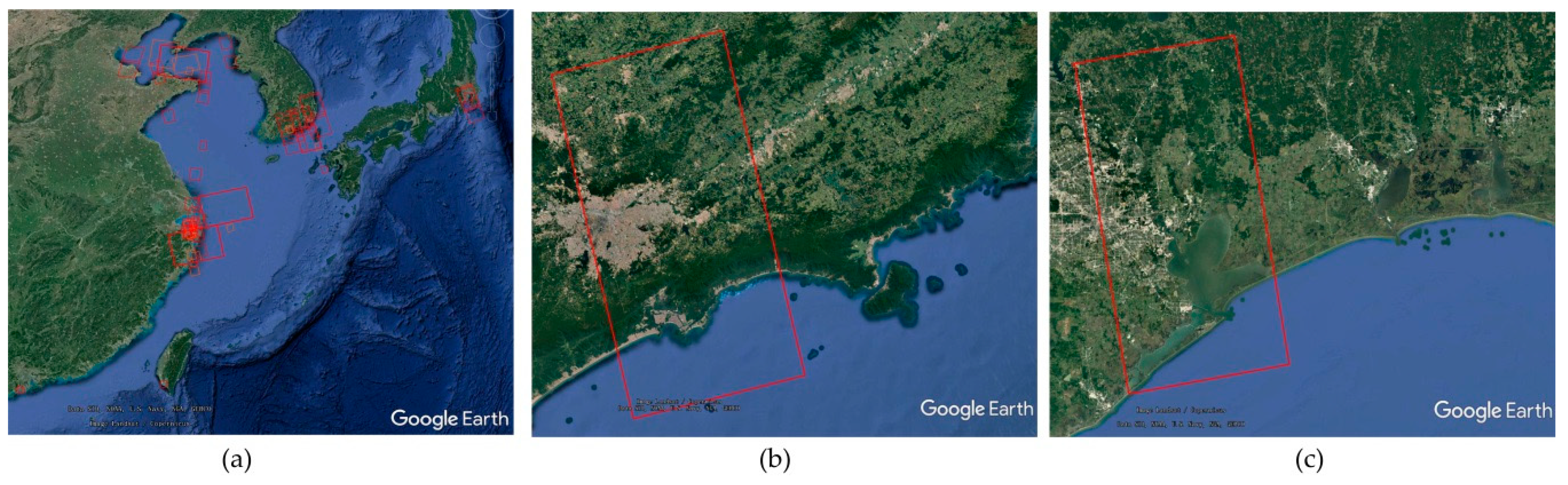
2.1. The Original SAR Image Dataset
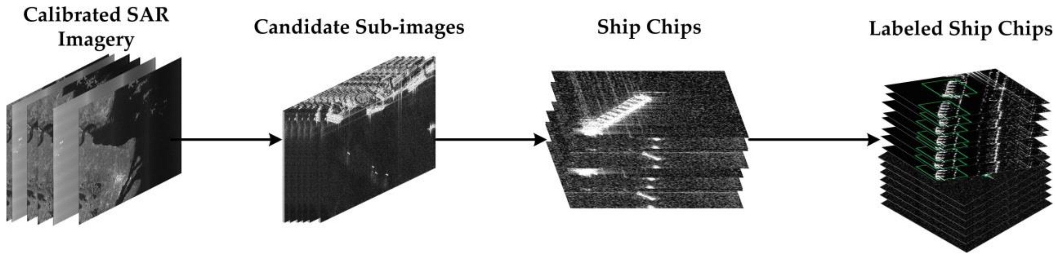
2.2. Policies for Construction of the Ship Detection Dataset
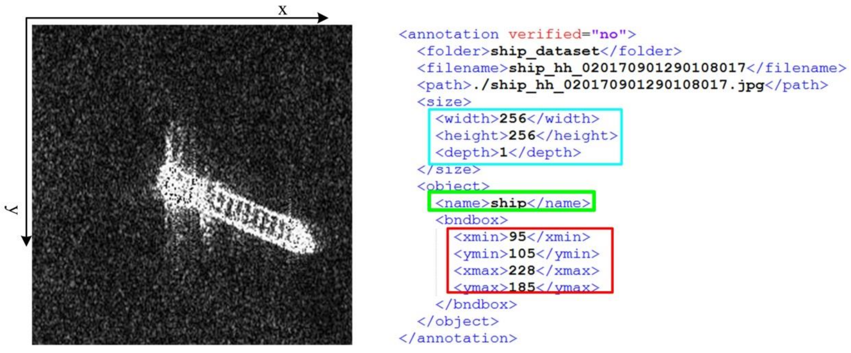
2.3. Properties of the Dataset
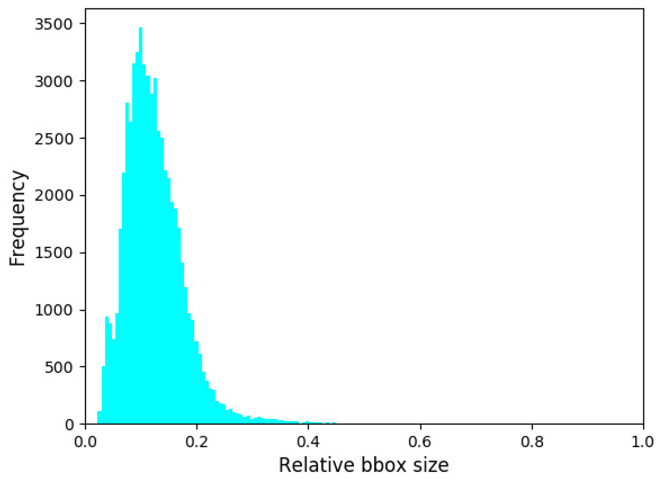
2.3.1. Multi-Scale Ship Size
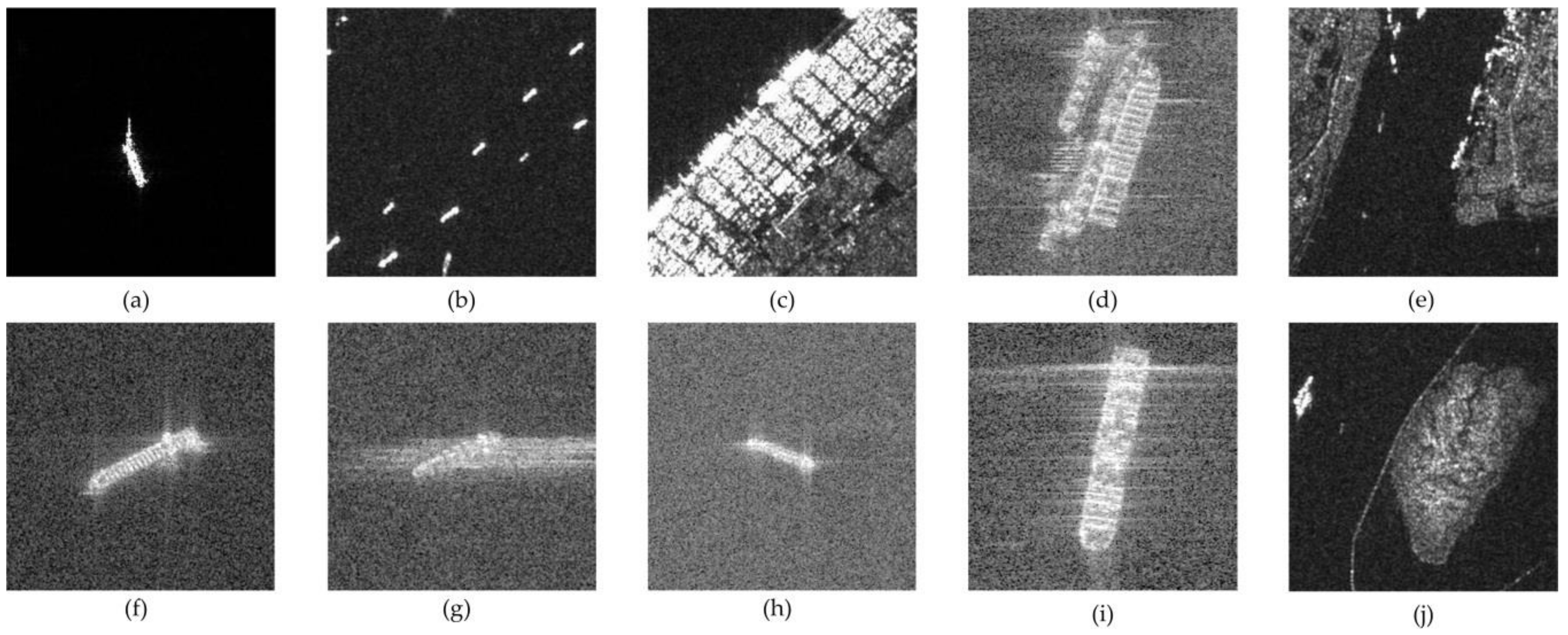
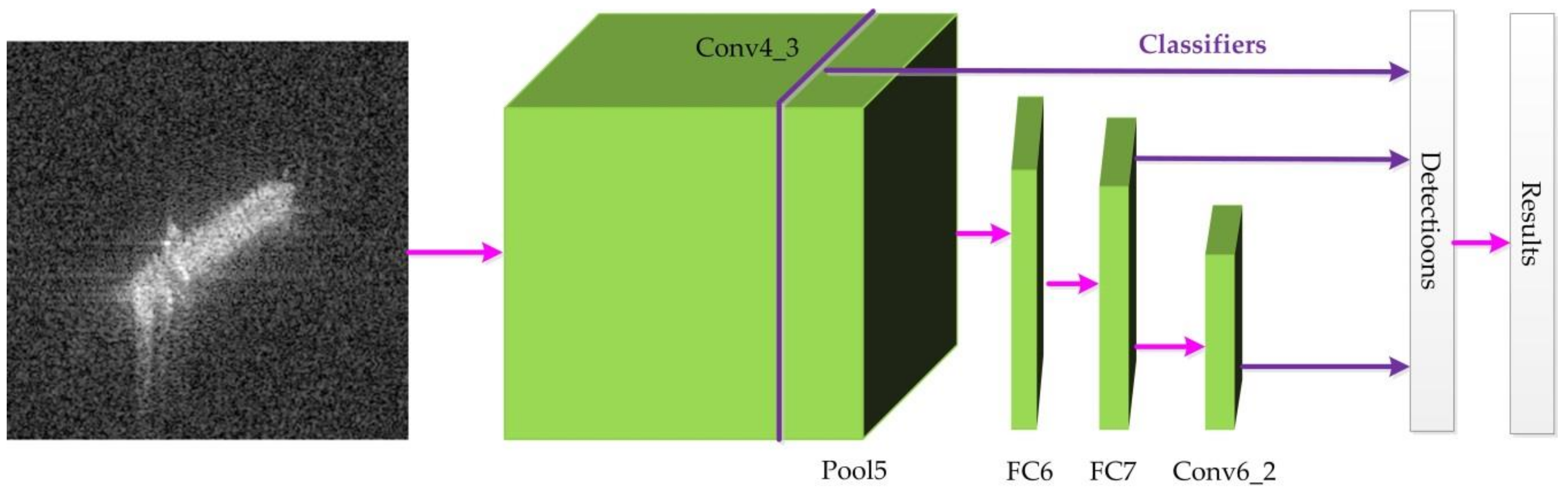
2.3.2. Complex Backgrounds for Ships
3. Experimental Results
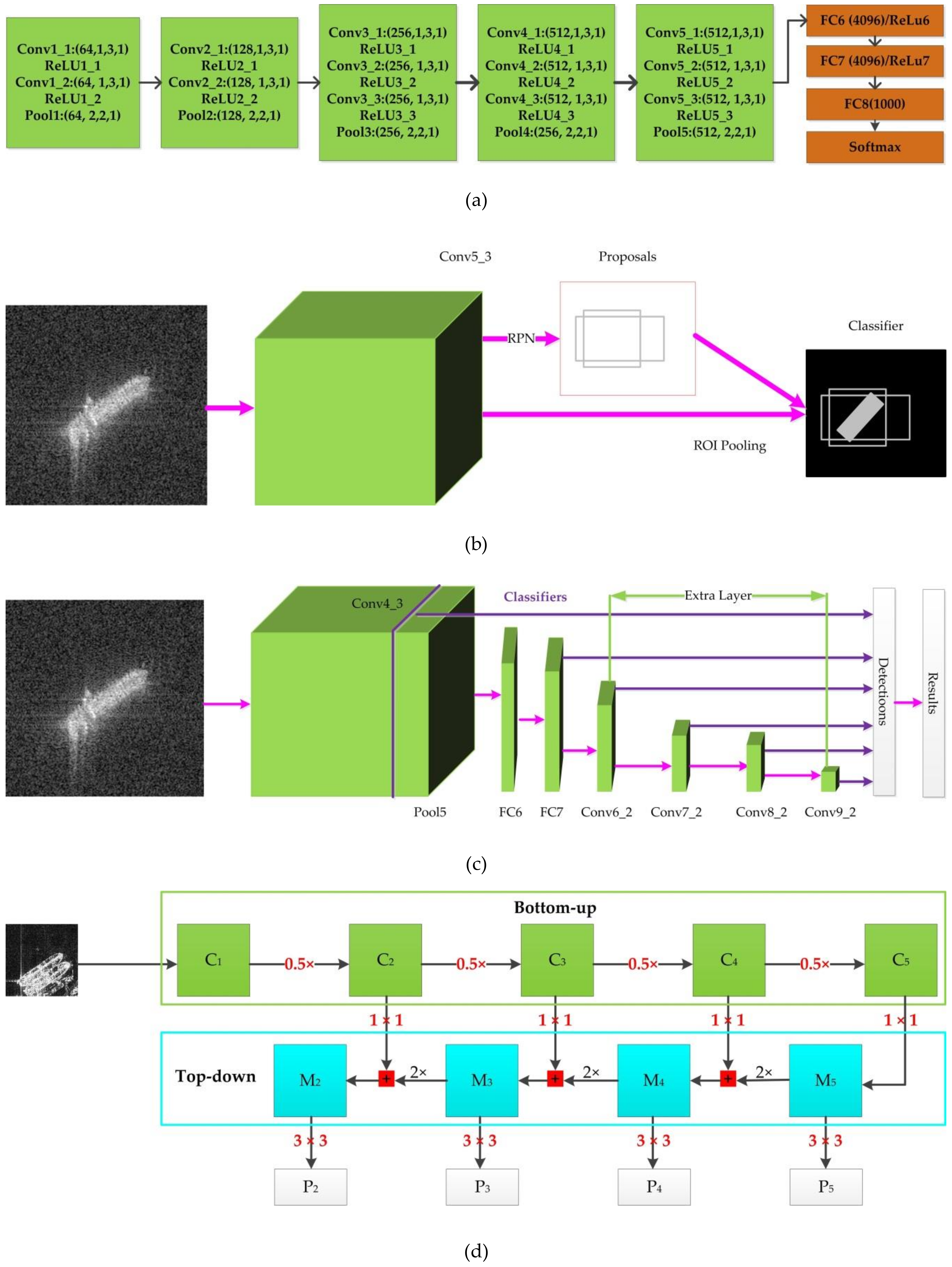
3.1. Related Object Detectors
3.1.1. VGG16
3.1.2. Faster R-CNN
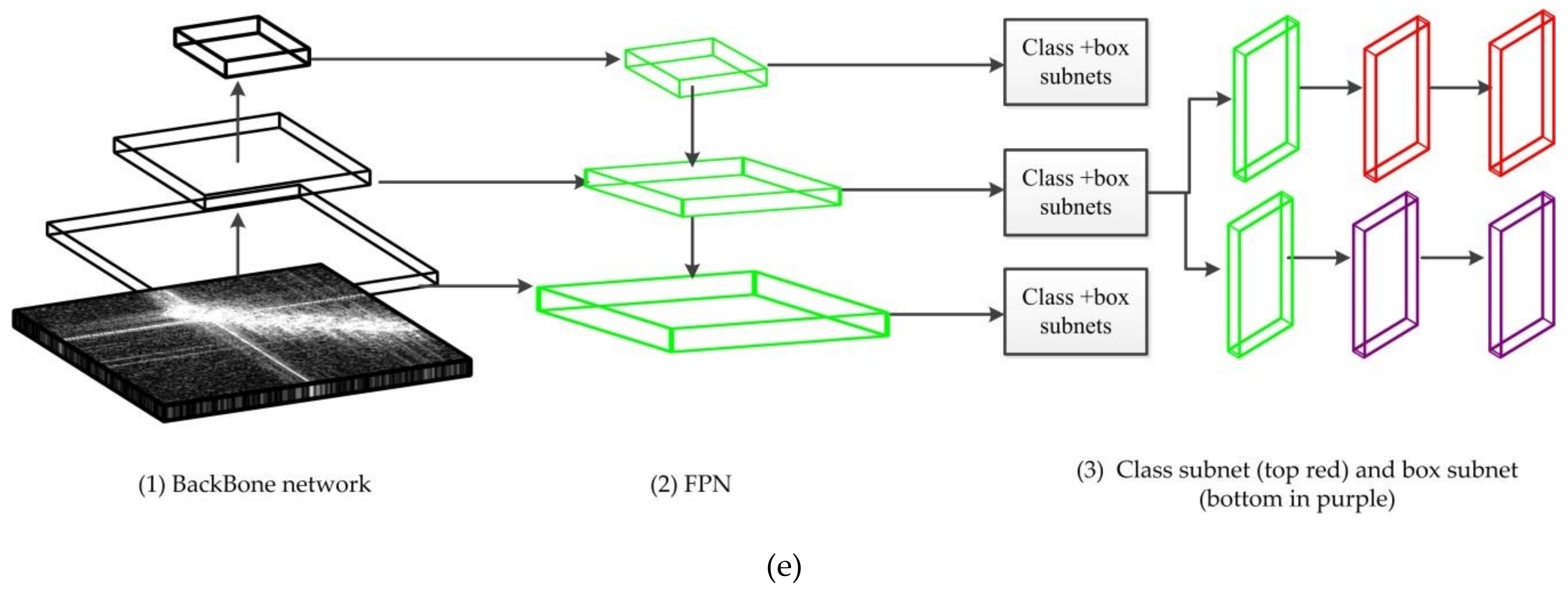
3.1.3. SSD
3.1.4. RetinaNet
3.2. Training Details
3.3. Experimental Results and Analysis
3.3.1. Experimental Results for Baselines
3.3.2. Experimental Results for Generalization
4. Discussion
5. Conclusions
Author Contributions
Funding
Acknowledgments
Conflicts of Interest
References
- El-Darymli, K.; McGuire, P.; Power, D.; Moloney, C.R. Target detection in synthetic aperture radar imagery: A state-of-the-art survey. J. Appl. Remote Sens. 2013, 7, 7–35. [Google Scholar]
- El-Darymli, K.; Gill, E.W.; Mcguire, P.; Power, D.; Moloney, C. Automatic Target Recognition in Synthetic Aperture Radar Imagery: A State-of-the-Art Review. IEEE Access 2016, 4, 6014–6058. [Google Scholar] [CrossRef]
- Kanjir, U.; Greidanus, H.; Oštir, K. Vessel detection and classification from spaceborne optical images: A literature survey. Remote Sens. Environ. 2018, 207, 1–26. [Google Scholar] [CrossRef]
- Dudgeon, D.E.; Lacoss, R.T. An Overview Ofautomatic Target Recognition; The College of Information Sciences and Technology: University Park, PA, USA, 1993. [Google Scholar]
- Crisp, D.J. The state-of-the-art in ship detection in Synthetic Aperture Radar imagery. Org. Lett. 2004, 35, 2165–2168. [Google Scholar]
- Ouchi, K. Current status on vessel detection and classification by synthetic aperture radar for maritime security and safety. In Proceedings of the 38th Symposium on Remote Sensing for Environmental Sciences, Gamagori, Aichi, Japan, 3–5 September 2016; pp. 5–12. [Google Scholar]
- Moreira, A.; Prats-Iraola, P.; Younis, M.; Krieger, G.; Hajnsek, I.; Papathanassiou, K.P. A tutorial on synthetic aperture radar. IEEE Geosci. Remote Sens. Mag. 2013, 1, 6–43. [Google Scholar] [CrossRef]
- Oliver, C.; Quegan, S. Understanding Synthetic Aperture Radar Images; SciTech Publ.: Chennai, India, 2004. [Google Scholar]
- European Space Agency. Sentinel-1 User Handbook; European Space Agency: Paris, France, 2013. [Google Scholar]
- Bi, F.; Liu, F.; Gao, L. A Hierarchical Salient-Region Based Algorithm for Ship Detection in Remote Sensing Images. In Advances in Neural Network Research and Applications; Zeng, Z., Wang, J., Eds.; Springer: Berlin/Heidelberg, Germany, 2010; pp. 729–738. [Google Scholar] [CrossRef]
- Huang, X.; Yang, W.; Zhang, H.; Xia, G.-S. Automatic Ship Detection in SAR Images Using Multi-Scale Heterogeneities and an A Contrario Decision. Remote Sens. 2015, 7, 7695–7711. [Google Scholar] [CrossRef]
- Pan, Z.; Liu, L.; Qiu, X.; Lei, B. Fast Vessel Detection in Gaofen-3 SAR Images with Ultrafine Strip-Map Mode. Sensors 2017, 17, 1578. [Google Scholar] [CrossRef]
- An, Q.; Pan, Z.; You, H. Ship Detection in Gaofen-3 SAR Images Based on Sea Clutter Distribution Analysis and Deep Convolutional Neural Network. Sensors 2018, 18, 334. [Google Scholar] [CrossRef]
- Kang, M.; Leng, X.; Lin, Z.; Ji, K. A modified faster R-CNN based on CFAR algorithm for SAR ship detection. In Proceedings of the 2017 International Workshop on Remote Sensing with Intelligent Processing (RSIP), Shanghai, China, 18–21 May 2017; pp. 1–4. [Google Scholar]
- Li, J.; Qu, C.; Shao, J. Ship detection in SAR images based on an improved faster R-CNN. In Proceedings of the 2017 SAR in Big Data Era: Models, Methods and Applications (BIGSARDATA), Beijing, China, 13–14 November 2017; pp. 1–6. [Google Scholar]
- Kang, M.; Ji, K.; Leng, X.; Lin, Z. Contextual Region-Based Convolutional Neural Network with Multilayer Fusion for SAR Ship Detection. Remote Sens. 2017, 9, 860. [Google Scholar] [CrossRef]
- Ball, J.E.; Chan, C.S. Comprehensive survey of deep learning in remote sensing: Theories, tools, and challenges for the community. J. Appl. Remote Sens. 2017, 11, 042609. [Google Scholar] [CrossRef]
- Zhu, X.X.; Tuia, D.; Mou, L.; Xia, G.S.; Zhang, L.; Xu, F.; Fraundorfer, F. Deep Learning in Remote Sensing: A Comprehensive Review and List of Resources. IEEE Geosci. Remote Sens. Mag. 2017, 5, 8–36. [Google Scholar] [CrossRef]
- Liu, Y.; Zhang, M.H.; Xu, P.; Guo, Z.W. SAR ship detection using sea-land segmentation-based convolutional neural network. In Proceedings of the 2017 International Workshop on Remote Sensing with Intelligent Processing (RSIP), Shanghai, China, 18–21 May 2017; pp. 1–4. [Google Scholar]
- Wang, Y.; Wang, C.; Zhang, H. Combining a single shot multibox detector with transfer learning for ship detection using sentinel-1 SAR images. Remote Sens. Lett. 2018, 9, 780–788. [Google Scholar] [CrossRef]
- Goodfellow, I.; Bengio, Y.; Courville, A. Deep Learning; MIT Press: Cambridge, MA, USA, 2016. [Google Scholar]
- Deng, J.; Dong, W.; Socher, R.; Li, L.; Kai, L.; Li, F.-F. ImageNet: A large-scale hierarchical image database. In Proceedings of the 2009 IEEE Conference on Computer Vision and Pattern Recognition, Miami, FL, USA, 20–25 June 2009; pp. 248–255. [Google Scholar]
- TsungYi, L.; Michael, M.; Serge, B.; James, H.; Pietro, P.; Deva, R.; Piotr, D.; Zitnick, C.L. Microsoft COCO: Common Objects in Context. In Computer Vision—ECCV 2014, Proceedings of the European Conference on Computer Vision, Zurich, Switzerland, 6–12 September 2014; Springer: Cham, Switzerland, 2014; Volume 8693, pp. 740–755. [Google Scholar]
- Zhang, Q. System Design and Key Technologies of the GF-3 Satellite. Acta Geod. Cartogr. Sin. 2017, 46, 9. [Google Scholar]
- SAR-Ship-Dataset. Available online: https://github.com/CAESAR-Radi/SAR-Ship-Dataset (accessed on 3 March 2019).
- Ren, S.; He, K.; Girshick, R.; Sun, J. Faster R-CNN: Towards Real-Time Object Detection with Region Proposal Networks. IEEE Trans. Pattern Anal. Mach. Intell. 2017, 39, 1137–1149. [Google Scholar] [CrossRef]
- Liu, W.; Anguelov, D.; Erhan, D.; Szegedy, C.; Reed, S.E.; Fu, C.-Y.; Berg, A.C. SSD: Single Shot MultiBox Detector. In Proceedings of the European Conference on Computer Vision (ECCV), Amsterdam, The Netherlands, 8–16 October 2016; pp. 21–37. [Google Scholar]
- Lin, T.; Goyal, P.; Girshick, R.; He, K.; Dollár, P. Focal Loss for Dense Object Detection. In Proceedings of the 2017 IEEE International Conference on Computer Vision (ICCV), Venice, Italy, 22–29 October 2017; pp. 2999–3007. [Google Scholar]
- LabelImg. Available online: https://github.com/tzutalin/labelImg (accessed on 6 May 2018).
- Everingham, M.; Gool, L.V.; Williams, C.K.I.; Winn, J.; Zisserman, A. The Pascal Visual Object Classes (VOC) Challenge. Int. J. Comput. Vis. 2010, 88, 303–338. [Google Scholar] [CrossRef]
- Xie, T.; Zhang, W.; Yang, L.; Wang, Q.; Huang, J.; Yuan, N. Inshore Ship Detection Based on Level Set Method and Visual Saliency for SAR Images. Sensors 2018, 18, 3877. [Google Scholar] [CrossRef] [PubMed]
- Horn, G.V.; Aodha, O.M.; Song, Y.; Cui, Y.; Sun, C.; Shepard, A.; Adam, H.; Perona, P.; Belongie, S.J. The INaturalist Species Classification and Detection Dataset. In Proceedings of the IEEE Conference on Computer Vision and Pattern Recognition, Salt Lake City, UT, USA, 18–22 June 2018; pp. 8769–8778. [Google Scholar]
- Girshick, R.; Donahue, J.; Darrell, T.; Malik, J. Rich Feature Hierarchies for Accurate Object Detection and Semantic Segmentation. In Proceedings of the IEEE Conference on Computer Vision & Pattern Recognition, Columbus, OH, USA, 24–27 June 2014. [Google Scholar]
- Lin, T.; Dollár, P.; Girshick, R.; He, K.; Hariharan, B.; Belongie, S. Feature Pyramid Networks for Object Detection. In Proceedings of the 2017 IEEE Conference on Computer Vision and Pattern Recognition (CVPR), Honolulu, HI, USA, 21–26 July 2017; pp. 936–944. [Google Scholar]
- Redmon, J.; Farhadi, A. YOLO9000: Better, Faster, Stronger. In Proceedings of the 2017 IEEE Conference on Computer Vision and Pattern Recognition (CVPR), Honolulu, HI, USA, 21–26 July 2017; pp. 6517–6525. [Google Scholar]
- Redmon, J.; Farhadi, A. YOLOv3: An Incremental Improvement. arXiv, 2018; arXiv:1804.02767. [Google Scholar]
- Simonyan, K.; Zisserman, A. Very Deep Convolutional Networks for Large-Scale Image Recognition. In Proceedings of the International Conference on Learning Representations (ICLR), San Diego, CA, USA, 7–9 May 2015. [Google Scholar]
- He, K.; Zhang, X.; Ren, S.; Sun, J. Deep Residual Learning for Image Recognition. In Proceedings of the 2016 IEEE Conference on Computer Vision and Pattern Recognition (CVPR), Las Vegas, NV, USA, 27–30 June 2016; pp. 770–778. [Google Scholar]
- Szegedy, C.; Wei, L.; Yangqing, J.; Sermanet, P.; Reed, S.; Anguelov, D.; Erhan, D.; Vanhoucke, V.; Rabinovich, A. Going deeper with convolutions. In Proceedings of the 2015 IEEE Conference on Computer Vision and Pattern Recognition (CVPR), Boston, MA, USA, 7–12 June 2015; pp. 1–9. [Google Scholar]
- Szegedy, C.; Vanhoucke, V.; Ioffe, S.; Shlens, J.; Wojna, Z. Rethinking the Inception Architecture for Computer Vision. In Proceedings of the 2016 IEEE Conference on Computer Vision and Pattern Recognition (CVPR), Las Vegas, NV, USA, 27–30 June 2016; pp. 2818–2826. [Google Scholar]
- Szegedy, C.; Ioffe, S.; Vanhoucke, V.; Alemi, A.A. Inception-v4, Inception-ResNet and the Impact of Residual Connections on Learning. In Proceedings of the Thirty-First AAAI Conference on Artificial Intelligence, San Francisco, CA, USA, 4–9 February 2017; pp. 4278–4284. [Google Scholar]
- Lin, T.; Goyal, P.; Girshick, R.; He, K.; Dollar, P. Focal loss for dense object detection. IEEE Trans. Pattern Anal. Mach. Intell. 2018. [Google Scholar] [CrossRef] [PubMed]
- Huang, G.; Liu, Z.; Maaten, L.v.d.; Weinberger, K.Q. Densely Connected Convolutional Networks. In Proceedings of the 2017 IEEE Conference on Computer Vision and Pattern Recognition (CVPR), Honolulu, HI, USA, 21–26 July 2017; pp. 2261–2269. [Google Scholar]
- Jia, Y.; Shelhamer, E.; Donahue, J.; Karayev, S.; Long, J.; Girshick, R.; Guadarrama, S.; Darrell, T. Caffe: Convolutional architecture for fast feature embedding. In Proceedings of the 22nd ACM international conference on Multimedia, Orlando, FL, USA, 3–7 November 2014; pp. 675–678. [Google Scholar]
- Tings, B.; Bentes, C.; Velotto, D.; Voinov, S. Modelling ship detectability depending on TerraSAR-X-derived metocean parameters. CEAS Space J. 2018. [Google Scholar] [CrossRef]
- Wang, Y.; Wang, C.; Zhang, H.; Dong, Y.; Wei, S. Automatic Ship Detection Based on RetinaNet Using Multi-Resolution Gaofen-3 Imagery. Remote Sens. 2019, 11, 531. [Google Scholar] [CrossRef]
- Hu, G.X.; Yang, Z.; Hu, L.; Huang, L.; Han, J.M. Small Object Detection with Multiscale Features. Int. J. Digit. Multimedia Broadcast. 2018, 2018, 10. [Google Scholar] [CrossRef]
- Cui, L. MDSSD: Multi-scale Deconvolutional Single Shot Detector for small objects. arXiv, 2018; arXiv:1805.07009. [Google Scholar]
- Guan, L.; Wu, Y.; Zhao, J. SCAN: Semantic Context Aware Network for Accurate Small Object Detection. Int. J. Comput. Intell. Syst. 2018, 11, 936–950. [Google Scholar] [CrossRef]
- Li, J.; Liang, X.; Wei, Y.; Xu, T.; Feng, J.; Yan, S. Perceptual Generative Adversarial Networks for Small Object Detection. In Proceedings of the IEEE Conference on Computer Vision and Pattern Recognition, Honolulu, HI, USA, 21–26 July 2017; pp. 1951–1959. [Google Scholar]


| Sensor | Imaging Mode | Resolution Rg. Az. (m) | Swath (km) | Incident Angle (°) | Polarization | Number of Images |
|---|---|---|---|---|---|---|
| GF-3 | UFS | 3 3 | 30 | 20~50 | Single | 12 |
| GF-3 | FS1 | 5 5 | 50 | 19~50 | Dual | 10 |
| GF-3 | QPSI | 8 8 | 30 | 20~41 | Full | 5 |
| GF-3 | FSII | 10 10 | 100 | 19~50 | Dual | 15 |
| GF-3 | QPSII | 25 25 | 40 | 20~38 | Full | 5 |
| Sentinel-1 | SM | 1.7 4.3 to 3.6 4.9 | 80 | 20~45 | Dual | 49 |
| Sentinel-1 1 | IW | 20 22 | 250 | 29~46 | Dual | 10 |
| Model | Input Size (pixels) | mAP (%) | Training Time (minutes) |
|---|---|---|---|
| SSD-300 | 300 300 | 88.32 | 193.25 |
| SSD-512 | 512 512 | 89.43 | 253.01 |
| Faster R-CNN | 600 800 | 88.26 | 531.4 |
| RetinaNet | 800 800 | 91.36 | 650.77 |
| Modified SSD-300 | 300 300 | 88.26 | 127.89 |
| Modified SSD-512 | 512 × 512 | 89.07 | 221.83 |
© 2019 by the authors. Licensee MDPI, Basel, Switzerland. This article is an open access article distributed under the terms and conditions of the Creative Commons Attribution (CC BY) license (http://creativecommons.org/licenses/by/4.0/).
Share and Cite
Wang, Y.; Wang, C.; Zhang, H.; Dong, Y.; Wei, S. A SAR Dataset of Ship Detection for Deep Learning under Complex Backgrounds. Remote Sens. 2019, 11, 765. https://doi.org/10.3390/rs11070765
Wang Y, Wang C, Zhang H, Dong Y, Wei S. A SAR Dataset of Ship Detection for Deep Learning under Complex Backgrounds. Remote Sensing. 2019; 11(7):765. https://doi.org/10.3390/rs11070765
Chicago/Turabian StyleWang, Yuanyuan, Chao Wang, Hong Zhang, Yingbo Dong, and Sisi Wei. 2019. "A SAR Dataset of Ship Detection for Deep Learning under Complex Backgrounds" Remote Sensing 11, no. 7: 765. https://doi.org/10.3390/rs11070765
APA StyleWang, Y., Wang, C., Zhang, H., Dong, Y., & Wei, S. (2019). A SAR Dataset of Ship Detection for Deep Learning under Complex Backgrounds. Remote Sensing, 11(7), 765. https://doi.org/10.3390/rs11070765