Article

Multispectral Transforms Using Convolution Neural Networks for Remote Sensing Multispectral Image Compression

1
Department of Engineering, University of Cambridge, 9 JJ Thomson Avenue, Cambridge CB3 0FA, UK
2
Optic Division, National Institute of Metrology, Beijing 100029, China
*
Author to whom correspondence should be addressed.
Remote Sens. 2019, 11(7), 759; https://doi.org/10.3390/rs11070759
Submission received: 23 January 2019 / Revised: 19 March 2019 / Accepted: 23 March 2019 / Published: 28 March 2019
(This article belongs to the Special Issue Convolutional Neural Networks Applications in Remote Sensing)

Abstract

:
A multispectral image is a three-order tensor since it is a three-dimensional matrix, i.e., one spectral dimension and two spatial position dimensions. Multispectral image compression can be achieved by means of the advantages of tensor decomposition (TD), such as Nonnegative Tucker Decomposition (NTD). Unfortunately, the TD suffers from high calculation complexity and cannot be used in the on-board low-complexity case (e.g., multispectral cameras) that the hardware resources and power are limited. Here, we propose a low-complexity compression approach for multispectral images based on convolution neural networks (CNNs) with NTD. We construct a new spectral transform using CNNs, where the CNNs are able to transform the three-dimension spectral tensor from large-scale to a small-scale version. The NTD resources only allocate the small-scale three-dimension tensor to improve calculation efficiency. We obtain the optimized small-scale spectral tensor by the minimization of original and reconstructed three-dimension spectral tensor in self-learning CNNs. Then, the NTD is applied to the optimized three-dimension spectral tensor in the DCT domain to obtain the high compression performance. We experimentally confirmed the proposed method on multispectral images. Compared to the case that the new spectral tensor transform with CNNs is not applied to the original three-dimension spectral tensor at the same compression bit-rates, the reconstructed image quality could be improved. Compared with the full NTD-based method, the computation efficiency was obviously improved with only a small sacrifices of PSNR without affecting the quality of images.

Graphical Abstract

1. Introduction

Multispectral images are acquired by a multispectral camera that is able to collect the reflected, emitted, or backscattered energy from an object or scene in multiple bands of the electromagnetic spectrum [1,2,3,4,5]. Multispectral images are considered the holy grail of observation tools in Earth observation because they can provide both spectral and spatial information of an object or scene. A multi-spectral camera is usually used as a payload of a satellite in multiple applications, such as monitor environments, surveying minerals, military targets, and so on [6,7,8,9]. Unfortunately, the information content of a multispectral image with large spatial and spectral information (high spectral and spatial resolution) [10,11] is much greater than the tolerance capabilities of current on-orbit available memory [12] and image-transmission downlink bandwidth of satellites. Therefore, it is helpful to compress remote sensing multispectral images without compromising quality.
Since multispectral images are three-dimensional, multispectral image compression fundamentally removes spatial and spectral redundancies, which is slightly different from panchromatic image compression, which only needs to remove spatial redundancies [13,14,15,16,17,18,19,20]. To achieve the fundamental target, many compression approaches for multispectral images have been developed [17,18,19,20,21,22,23,24,25,26,27,28,29]. To our best knowledge, multispectral image compression methods could be mainly summarized into three main categories: (1) prediction-based approaches [30]; (2) vector quantization approaches [31]; and (3) transform-based approaches [32]. Table 1 shows the comparison of different methods for multispectral images. Prediction-based methods are the earliest multispectral compression methods which are performed in a spatial or frequency domain, such as LUT [33], three-dimensional (3D) prediction, DPCM, and CCSDS-MDC [34]. The main advantage of the prediction-based approaches is their low complexity. These methods are lossless compression. Currently, these methods are also extended as a part of other compression algorithms, such as CCSDS-IDC. The main disadvantages of the prediction-based approaches are low compression performance and their weak fault-tolerance ability. Vector quantization approaches (using the quantization technique) involves two parts: grouping vectors and quantizing vector. The vector quantization approaches use a training method to group a large set of vectors. Thus, it is difficult to become a fast algorithm, i.e., this method is not easy to implement on a hardware platform. A transform-based method is a frequency domain method, where the compression task is performed in the transformed domain. First, a 3D transform (e.g., 3DWT, 3DCT, Karhunen–Loeve Transform + Discrete Wavelet Transform (KLT + 2DWT), and KLT+post wavelet transform) is able to regroup the energy distribution in a transform domain. Second, existing encoders (e.g., bit-plane coding or entropy encoding methods) process the transformed coefficients. This method has many advantages, such as high compression performance, high fault-tolerance performance, and the possibility of fast calculations. Thus, the transform-based approach is widely used in multispectral images and other images (e.g., panchromatic images) on the ground or on-board cases. From the 3D data inherent structure aspect, the transform-based approaches may crush the inherent structure of a multispectral image and mask redundancy information, which would result in the high-order dependencies that still existed in images because the compression process regards the multispectral image as a matrix.
To exploit the high-order dependencies, tensor decomposition methods are recently applied to compression of multispectral images [35,36,37,38,39]. A multispectral image is able to regard a three-order tensor. The compression results could be achieved by a Tucker Decomposition (TD) approach. Karami et al. used TD in conjunction with 3D-DCT to compress hyper-spectral images. The 3D-DCT+TD approaches could reach 38–22 dB at 10–100 of CR, which is able to improve 3 dB and 4 dB compared to only TD and only 3D-DCT [35]. Karami et al. [36] combined DWT and TD to compress hyper-spectral images. The experimental results show that this approach could reach 49.5–58.1 dB for Cuprite at 0.05–1 bpp, and 40.1–55.3 dB for Moffett Field at 0.05–1 bpp. Moreover, this method gains higher PSNR compared with Principal Components Analysis (PCA) + JPEG2000 and 2D Set Partitioned Embedded Block Coder (SPECK). These two investigations indicate that the TD-based approach is able to gain better compression performance for multispectral image compression. Unfortunately, this method suffers high calculation complexity (see Table 1) and conflicts with the low-complexity requirements of on-board multispectral cameras.
In our previous works, we investigated the tensor decomposition compression methods to achieve low complexity. In [40], Tucker decomposition is applied to multispectral images with comparatively few bands in the post-transform domain. In [41], an accelerated nonnegative tensor decomposition (i.e., a pair-wise multilevel grouping approach) for hyperspectral image compressions was developed. This method is able to reduce the calculation complexity through the slight sacrifice of the compression performance.
In this work, we propose a new spectral tensor transform using convolutional neural networks (CNNs) to reduce the computational complexity of a large-scale tensor decomposition. We use the constructed spectral tensor transform in conjunction with nonnegative tensor decomposition (NTD) in the DCT domain to compress multispectral images, which is able to reduce the total resources utilization of tensor decomposition. This method focuses on transforming large-scale spectral tensors into the small-scale version. NTD resources are only allocated to small-scale spectral tensor in the DCT domain; thus, the low computation complexity is achieved. By means of exploiting the compact spectral information hidden in multispectral image tensor, this method uses the relatively small total NTD resources are, which can achieve efficient calculations.
The remainder of the paper is organized as follows. Section 2 presents the proposed compression framework, including the compression principle of NTD, the spectral transform of the CNNs, and the compression scheme. Experimental results are reported in Section 3. In Section 4, we conclude this paper.

2. Materials and Methods

In Section 2.1, we present the principle of multispectral compression based on NTD, followed in Section 2.2 by the proposed spectral transform of the CNNs. Finally, Section 2.3 demonstrates the proposed compression scheme using the CNNs.

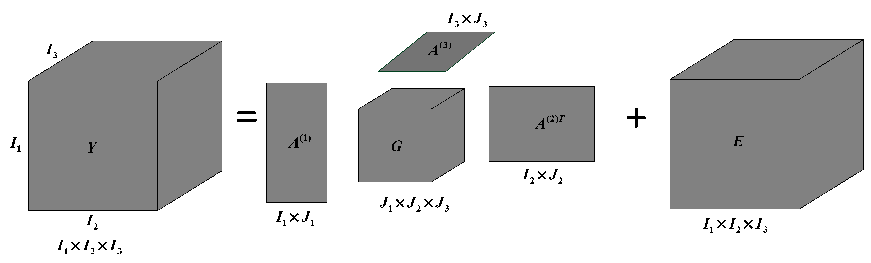
2.1. NTD for Multispectral Compression

A multispectral image is a 3D matrix and fundamentally includes both spatial redundancy and spectral redundancy. The multispectral compression aims at removing both redundancies. Figure 1 shows the general principle for multispectral compression using NTD approaches. The NTD-based compression method involves three steps. In the first step, a two-dimensional (2D) transform (e.g., 2D-DWT and 2D-DCT) is utilized to remove spatial correlation in intra-band. In the second step, all transformed bands form a three-dimensional tensor. After that, a Tucker Decomposition is applied to the three-dimensional tensor to generate a core tensor and several factor matrixes. In the last step, an adaptive arithmetic encoder is used to process the core tensor and factor matrixes.
A tensor is a multi-way array or multi-dimensional matrix. We use Y R I 1 × I 2 × I 3 to express a three-dimensional tensor, where each element is a transformed coefficient. Here, I 1 × I 2 × I 3 is the dimension of the tensor Y . The decomposition of a three-dimensional tensor is that a given tensor is decomposed into three component (or factor) matrixes. We provide the important notations shown in Table 2 to demonstrate the principle of the three-dimensional tensor decomposition. When a Tucker decomposition (also called the best rank approximation) is applied to the three-dimensional tensor, a low-dimension core tensor and several factor matrixes are generated [42]. Here, the low-dimension core tensor is denoted by G R J 1 × J 2 × J 3 ( J 1 × J 2 × J 3 is the dimension of the tensor G). Factor matrixes are denoted by A ( n ) = [ a 1 ( n ) , a 2 ( n ) , , a J n ( n ) ] R I n × J n   ( n = 1 , 2 , 3 ) . Given a tensor Y , a core tensor G and three-component matrixes A ( n ) are found, which perform the following approximate decomposition:
A = j 1 = 1 J 1 j 2 = 1 J 2 j 3 = 1 J 3 g j 1 j 2 j 3 a j 1 ( 1 ) a j 2 ( 2 ) a j 3 ( 3 ) + E = G × 1 A ( 1 ) × 2 A ( 2 ) × 3 A ( 3 ) + E = G × { A } + E = Y ^ + E Y ^
where E is an estimation error of tensor Y in the decomposition process, and Y ^ is an equivalent tensor (i.e., approximately evaluated tensor) using the generated core tensor and factor matrixes. Figure 2 shows the graphic illustration of the Tucker Decomposition of Equation (1) on the three-dimensional tensor.
To achieve Equation (1), the Tucker decomposition is a search process for the optimal core tensor and factor matrixes to make the minimized residual error tensor.
min 1 2 Y G × 1 A ( 1 ) × 2 A ( 2 ) × 3 A ( 3 ) F 2 s . t . G R J 1 × J 2 × J 3 , A ( n ) R I n × J n , n = 1 , 2 , 3
The Tucker decomposition is able to achieve the compression results because original high dimension tensor is able to become into a lower dimension core tensor. The tensor decomposition is performed on the whole multispectral image, which means it can simultaneously remove the spectral and residual spatial redundancies. Here, we use a fast algorithm based on HALS-NTD [43,44] to implement the Tucker decomposition. The important notations of the decomposition algorithm with HALS-NTD are in Table 3. Algorithm 1 shows the HALS-NTD to process a three-order tensor. In Algorithm 1, Step 11 and Step 16 are the learning rules for NTD factors A and core tensor G. The detailed explanations of the learning rules can be found in [43,44].
Algorithm 1 [43,44]:
1: Input: a given tensor Y , its size is I 1 × I 2 × × I N ,   N = 3 ;
    The core tensor size is J 1 × J 2 × J N .
2: Output: a core tensor G R J 1 × J 2 × J N ,
    N factors A ( n ) = [ a 1 ( n ) , a 2 ( n ) , , a J n ( n ) ] R + I n × J n .
3: Begin
4: Initializing G and all A ( n ) .
5: Normalizing all a j n ( n ) for n = 1, 2, …, N to unit length.
6: Calculating the residual tensor as E = Y Y ^ .
7: Repeat
8: for n = 1 to N do
9: for jn = 1 to jn = Jn do
10: Calculate prediction tensor: Y ( n ) ( j n ) = E ( n ) + a j n ( n ) [ G ( n ) ] j n A n T
11: Update factors: a j n ( n ) [ Y ( n ) ( j n ) [ ( G × n { A } ) ( n ) ] j n T ] +
12: Normalizing factors: a j n ( n ) a j n ( n ) a j n ( n ) p
13: Update errors: E n Y ( n ) ( j n ) a j n ( n ) [ G ( n ) ] j n A n T
14: End
15: End
16: Update core tensor: G [ G ( Y Y ^ ) × { A T } ] +
17: For each j1 = 1, …, J1, j2 = 1, …, J2, …, jN = 1, …, JN do
18: Calculate core tensor:
g j 1 j 2 , j N g j 1 j 2 , j N + E × 1 a j 1 ( 1 ) × 2 a j 2 ( 2 ) × N a j N ( N )
19: Calculate error tensor:
E E + Δ g j 1 j 2 , j N a j 1 ( 1 ) a j 2 ( 2 ) a j N ( N )
20: End
21: Until the converge condition is achieved.
22: End
23: Return G and A ( n ) .

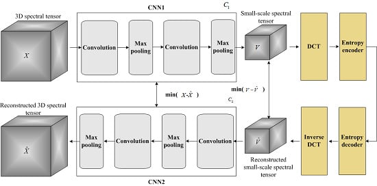
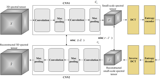
2.2. Proposed Multispectral Tensor with CNNs

Here, we propose an efficient spectral tensor transform method using convolution neural networks to compress remote sensing multispectral image tensors. Different from the traditional NTD method directly applied to a large-scale original multispectral tensor representation, the proposed concept is that the use of a learning network transforms the original large-scale spectral tensor into the small-scale version. Then, the NTD is applied to the small-scale spectral tensor in the DCT domain. Thus, the total NTD resources are relatively small, which can achieve efficient calculation. Considering that the transform is an unsupervised learning task, we construct a self-learning network using two convolution neural networks. Figure 3 shows the spectral transform schematic of convolution neural networks.
Here, the CNN in the forward channel is called the forward CNN. Accordingly, the CNN in the backward channel is called the backward CNN. We use X N to express a multispectral three-dimension tensor, which is the input of the forward CNN. The first step of the CNN is a convolution operation between X and a filter with m1 learned filters having the length of n0. The convolution can be modeled using a matrix multiplication as
X 1 = W 1 T X
where W1 is the convolution filter of the first layer and X1 is the created feature map. In the second step, a nonlinear function is applied to the created feature map to obtain the first layer CNN feature denoted by Z1, which can be expressed as:
Z 1 = Ψ ( W 1 T X )
where Ψ can be implemented using a Rectifier Linear Unit (ReLU), Ψ ( t ) = max ( t , 0 ) . The second layer can be obtained as the same method as:
Z 2 = Ψ [ W 2 T Z 1 ] = Ψ [ W 2 T Ψ ( W 1 T X ) ]
where W2 is the convolution filter of the first layer. Using the same principle, other layers can be obtained. The nth layer can be expressed as:
Z n = Ψ [ W n T Z n 1 ]
We use the C1 (·) to express the whole operation model of the forward CNN. We use V to express the resultant representation through the CNN. Equation (6) of the forward CNN can be expressed as:
V = C 1 ( W , X )
where W is the filter parameter of the forward CNN. The DCT transform is applied to the resultant representation from the forward CNN, where the calculation model can be expressed as
F = D T ( V ) = B V B T
where DT(·) express the DCT transform, B is the DCT basis.
To obtain the optimized features, i.e., V , we add the back-forward channel constituting an inverse DCT transform and a CNN. Moreover, the DCT transform basis is an orthogonal basis, which means B−1 = BT. The backward CNN can be expressed by X ^ = C2(U, V ^ ), where U is the filter parameter of the CNN and C2 (·) is the calculation function of the CNN. V ^ is the inverse DCT transform signal, V ^ = DT−1(F). The back-forward calculation model can be expressed as
X ^ = C 2 ( U , V ^ ) = C 2 ( U , D T 1 ( F ) ) = C 2 ( U , B T F B )
where C 2 ( ) is the calculation model of the backward CNN in the back-forward channel. To obtain the best wavelet representation (i.e., V ), we minimize the error between the input X signal and the reconstructed X ^ to perform the learning goal as
H ( W ^ , U ^ ) = arg min W , U C 2 ( U , D T 1 ( D T ( C 1 ( W , X ) ) ) ) X 2 2
To fast solve Equation (10), we use an alternate iteration concept, which can be divided into two steps:
Step 1:
W ^ = arg min W C 2 ( U ^ , D T 1 ( D T ( C 1 ( W , X ) ) ) ) X 2 2 + λ 1 W 2 2
Step 2:
U ^ = arg min U C 2 ( U , D T 1 ( D T ( C 1 ( W ^ , X ) ) ) ) X 2 2 + λ 2 U 2 2
where λ1 and λ2 are the regularization parameters. To efficiently calculate W ^ and U ^ , here, we use Equations (13) and (14) to replace Equations (11) and (12) by adding a regularization term as:
Step 1:
W ^ = arg min W C 2 ( U ^ , ( C 1 ( W , X ) ) ) X 2 2 + λ 1 W 2 2 + β 1 C 1 ( W , X ) D T 1 ( D T ( C 1 ( W , X ) ) ) 2 2
Step 2:
U ^ = arg min U C 2 ( U , V ^ ) X 2 2 + λ 2 U 2 2 + β 2 C 1 ( W ^ , X ) V ^ 2 2
where β1 and β2 are the regularization parameters. The detailed derivation procedure from Equations (11) and (12) to Equations (13) and (14) can be seen in Appendix A. The two-step learning algorithm of the multispectral transform can be summarized, as given below, which is used to obtain the best small-scale spectral tensor and CNN parameters. By the new spectral tensor transform with two CNNs, the best small-scale spectral tensor can be obtained. The best small-scale spectral tensor is a small-scale version of the original large-scale spectral tensor, which is able to preserve structural information of the original spectral tensor, has a small size and therefore is able to reduce the utilization of the total NTD resources.
Algorithm 2: Spectral tensor transform using two CNNs
1: Input: The original spectral tensor, denoted by X;
2: Output: The learnable parameters of two CNNs W ^ , U . The best small-3: scale spectral tensor V ^
3: Initialization: initial learnable parameters, W ^ 0 , U ^ 0 for two CNNs, alternate iteration number k = 0.
4: While do {
5: k = k + 1;
6: Step 1:
7: V = V ^ k
8: Update U k by training the backward CNN to compute Equation (14).
9: Step 2:
10: U = U ^ k
11: Update W ^ k by training the forward CNN to compute Equation (13).
12: Until iteration condition is met, here, the iteration condition is k = K.
13: Return: V ^ = V ^ k , U = U ^ k , W ^ = W ^ k

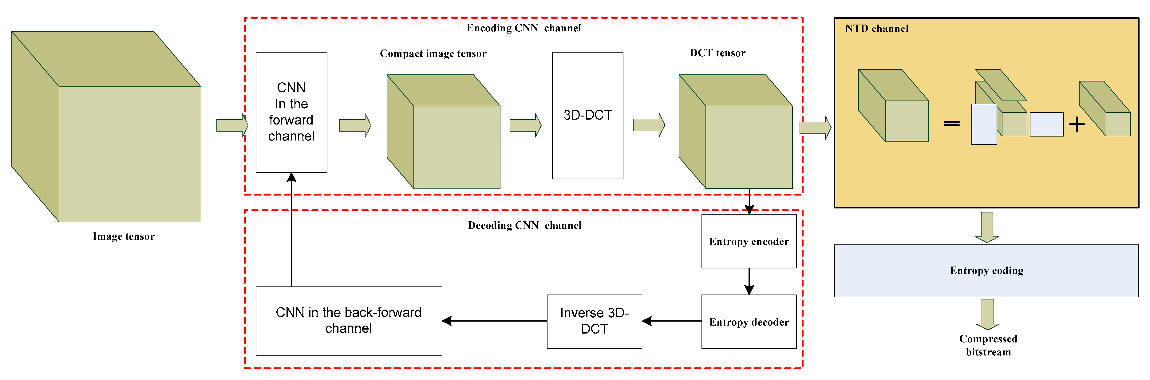
2.3. Proposed Multispectral Compression Scheme with CNNs

We use CNNs and NTD to construct an image compressor to obtain both low-complexity and high compression performance. The overall architecture of the proposed compression approach is shown in Figure 4. The overall architecture of the whole algorithm includes three parts: an encoding CNN channel, a decoding CNN channel, and an NTD channel. The encoding CNN channel and decoding CNN channel form a closed-loop link to train the filter parameters of two CNNs. First, multispectral training images are input to the closed-loop link. The two-step algorithm (i.e., Algorithm 2) is performed to obtain the optimized filter parameters of two networks. Second, a multispectral image passes through the encoding CNN channel, NTD channel, and Entropy coding unit to complete the compression task. In the encoding CNN channel, a CNN firstly transforms the large-scale image representation into small-scale features (i.e., compact image tensors). After that, a 3D-DCT is applied to the small-scale image tensors to obtain the DCT tensors. The NTD channel performs the NTD process and completes the final encoding in connection with entropy encoders. When the decompression task is required, the compressed bit-streams can be used to reconstruct the original multispectral images via the decoding CNN channel. The decoding CNN channel has two functions. The first is that the use of another CNN helps the encoding channel’s CNN to obtain the best small-scale wavelet representation. The second is that it is used to decode compressed bit-streams when a reconstruction task is required.
Given the training data S of input-target pairs { X ( m ) , U ^ } , the first CNN proceeds by minimizing the mean squared error (MSE) between the reconstructed spectral image via the second CNN and original spectral image as
g 1 ( W ) = 1 M S X ( m ) S X ^ ( m ) X ( m ) 2 2 + λ 1 W 2 2 + β 1 C 1 ( W , X ) D T 1 ( D T ( C 1 ( W , X ) ) ) 2 2
where X ^ ( m ) = C 2 ( U ^ , C 1 ( W , X ( m ) ) ) , W is the learnable parameter of the first CNN, U ^ is the learnable parameter of the second CNN, X is the original image representation, and M S is the number of samples in the training set S. In Equation (15), U ^ and X are input parameters. Accordingly, the loss function of the second CNN can be expressed as:
g 2 ( U ) = 1 M S X ( m ) S C 2 ( U , V ^ ) X ( m ) 2 2 + λ 2 U 2 2 + β 2 C 1 ( W ^ , X ) V ^ 2 2
where V ^ is the small-scale feature from the first CNN. The best small-scale image representation is obtained by the error minimization between the original and reconstructed image representations in the two CNNs. Then, the small-scale image representation is also further transformed to small-scale DCT tensor using the 3D-DCT. This is done to remove the spatial and spectral correlation. The small-scale DCT tensor is decomposed by the NTD method. In the DCT domain, the NTD is applied to remove residual spatial correlation and spectral correlation. Finally, an entropy encoding completes the final encoding task. The learned convolution filter from two CNN can be used as the side information of the compressor.
In the NTD channel, we use a multilevel decomposition (MD) method to implement the fast NTD method. Here, we take the band number of 32 as an example to demonstrate the MD principle. Figure 5 shows the MD principle when the band number is 32. The process level number is 3. In the first level, there are eight sub-tensors. Each sub-tensor is processed by TD to produce core tensor and three-factor matrixes. In the second level, every four core tensors produced in the first level are considered as a new tensor. There are the regrouped tensors. Each tensor is processed by TD. In the third level, the two core tensors produced in the first level are considered as a new tensor, which is processed by TD. Finally, one core tensor and several factor matrixes are produced.
We use F = { f η , ρ } to express a spectral group in multilevel TD structure. Here, η is the decomposition level, and ρ is the tensor order of in F. In F , the jth tensor in the level i is denoted as f i , j . Let S ( f i , j ) be the size of the current tensor f i , j . Let T h ( f i , j ) be the size of core tensor decomposed in the current level. S ( f i , j ) is equal to J 1 , i , j × J 2 , i , j × J 3 , i , j in the ith level, and T h ( f i , j ) is the J 1 , i + 1 , j × J 2 , i + 1 , j × J 3 , i + 1 , j in next level. At each level, the resulted core tensor operates has the same the size of J 1 , i + 1 , j × J 2 , i + 1 , j × J 3 , i + 1 , j , j = 1, 2, …, J. The size J 1 , i + 1 , j × J 2 , i + 1 , j × J 3 , i + 1 , j of core tensor in each level could be determined by the compression bit-rate. In all levels of TD, the different level has different the size of the core tensor. Let G ( f i , j ) express the resulted core tensor f i , j . The adjacent tensor relationship is as follows:
f 2 , 1 = G ( f 1 , 1 ) + G ( f 1 , 2 ) + G ( f 1 , 3 ) + G ( f 1 , 4 )
f 2 , 2 = G ( f 1 , 5 ) + G ( f 1 , 6 ) + G ( f 1 , 7 ) + G ( f 1 , 8 )
f 3 , 1 = G ( f 2 , 1 ) + G ( f 2 , 2 )
We allocate bit-rates to f i , j in F based on a l 1 norm approach. In the first level, the jth tensor allocated bit-rates can be expressed as:
f 1 , j = f 1 , j 1 j = 1 8 f 1 , j 1 × T t o a l l
where T t o a l l is total bit-rates. The other levels use the same way.

3. Results

To evaluate the compression performance of the proposed algorithm with the spectral transform using CNNs, we used MATLAB to perform the experiments on a personal computer (PC). The working parameters of the experimental PC are 3.6 GHz of CPU and 4 GB of memory. We tested our CNN-based NTD method on 50 multispectral images that consist of a variety of buildings, cities, and mountains. All 50 multispectral images were compressed by conforming to the following processing. First, each band of the original was 1024 × 1024 pixels. Second, the CNN-based spectral transform method was applied to the original spectral image to obtain the small-scale spectral tensor. Third, small-scale spectral tensor performed a DCT transform to remove spatial correlations. In the DCT domain, NTD was performed to remove the residual spectral and spatial correlations. Figure 6 shows the reconstructed multispectral image, where the bit-rates were set from 0.25 bpp to 2.0 bpp. Figure 7 shows the zoomed area of the fourth band, where the area was 100 × 100 pixels. With the increase of the bit-rates, the reconstruction quality gradually increased. From the subjective aspect, the reconstructed bands at the bit-rate of 2.0 bpp were very close to the original bands. As shown in the reconstructed images, the reconstructed images had better quality at the bit-rate of 0.25 bpp because our algorithm had better rate-distortion performance.
We objectively evaluated the proposed method by means of peak-signal-noise-ratio (PSNR), mean structural similarity (MSSIM), and visual information fidelity (VIF). In [36], the TD in the wavelet domain has the best compression performance, achieving a higher PSNR than PCA+jpeg2000 and 3D SPECK. We also used the conventional NTD to process all DCT coefficient blocks, where NTD resources were equally allocated to the large-scale DCT coefficient blocks. In addition, we used DWT+BPE as a reference method to process all wavelet coefficient blocks. The bit-rate was set to 0.5-3 bpp. Figure 8 show the test PSNR, MSSIM, and VIF using different methods.
The proposed algorithm on the experimental multispectral images was compared with PCA, SPIHT+2D-DWT with KLT [45], SPECK+2D-DWT [46] with KLT, and POT [47]. The average PSNR was considered as the PSNR of the corresponding method. The PSNR comparisons are demonstrated in Table 4. Due to the full usage of CNN and NTD in the DCT domain, the proposed compression achieved a good compression performance. The proposed method could improve PSNR by 0.46–1.63 dB against SPIHT+2D-DWT with KLT at 2–0.25 bpp.
Finally, we tested the compression time of the two methods. Figure 9 shows results of the comparison of the processing time of our algorithm and conventional NTD approaches. As shown in Figure 9, the proposed method was faster than conventional NTD method at different bit-rates. Figure 10 shows the comparison of compression performance and compression time at different bit-rates. As shown in Figure 10, the proposed method had a small sacrificing PSNR compared with conventional NTD method at different bit-rates. Table 5 shows the average improvement of the compression time and decrease of the compression performance. The computation efficiency of our compression approach improved 49.66% compared to traditional approaches while only sacrificing 0.3369 dB. The small sacrificing PSNR does not affect the quality of the images. These results indicate that our algorithm has low-complexity and high performance. This method has the possibility of spatial application.

4. Discussion

We discuss the proposed method from the following aspects, which is shown Table 6. As shown in Figure 8, Figure 9 and Figure 10, the compression performance of the proposed method was slightly lower than the traditional NTD. However, the proposed method improved the computation efficiency by 49.66%. In the traditional NTD method, the whole spectral tensor is directly decomposed by the NTD algorithm in the DCT domain. In the proposed method, the whole spectral tensor is processed from two compression steps. The first compression step is that the CNNs transforms a large-scale spectral tensor into a small-scale spectral tensor. The second compression step is that the NTD is applied to the small-scale spectral tensor. These two steps achieve a high compression performance. The sacrificing PSNR is firstly from the first step because the NTD and inverse NTD do not include the self-learning network. This is done because we consider the high calculation complexity of the NTD and inverse NTD. The sacrificing PSNR is also from the multi-level NTD. We also tested the compression performance of the CNNs with NTD and inverse NTD. We found that the compression performance was basically the same as the traditional NTD method. However, the calculation complexity was very high. Our current method performed a tradeoff between compression performance and complexity.
As shown in Figure 9 and Figure 10, the proposed method could improve the computation efficiency by 49.66% compared with the traditional NTD method. The calculation efficiency improvement was from two stages. The first stage is that we use the CNN to obtain a compact spectral tensor, which is actually a compression process. For the traditional NTD method, if it also obtains the same compact spectral tensor, a lot of calculation resources need to be used. The second stage is that we use a fast NTD method based on multilevel decomposition technologies. This stage is able to improve the decomposition speed of the three-order tensor. In the future, we will use hardware platforms, such as FPGA, DSP, and GPU, to implement the compression algorithm, where we will analyze the hardware resource utilization.
In the CNNs, the DCT and entropy encoder is used because our compression algorithm uses the DCT as the sparse representation tool and the entropy encoder as the entropy coding. In the self-learning network, we also use Hardmard Transform (HT) to replace the DCT. After obtaining the small-scale spectral tensors, we still use the DCT and NTD to remove the spatial and spectral correlations. We also multispectral images to perform the experiments when the different learning networks are used. Figure 11 shows the comparison of two different learning networks. The experimental results show the use of the HT-based CNNs obtained a lower PSNR (i.e., lower compression performance) than the proposed method. Thus, the sparse represent method and entropy encoder in the convolution neural learning network need to keep the same to the latter stage of the compression methods.

5. Conclusions

In this paper, we propose a low-complexity but efficient compression approach based on the convolution neural networks in conjunction with NTD for multispectral images. First, we use two convolution neural networks to construct a new spectral transform. The new spectral transform can transform a large-scale three-dimension spectral tensor into a small-scale three-dimensional spectral tensor. We obtain the optimized small-scale spectral tensor by the minimization of original and reconstructed three-order spectral tensor in CNNs. The new spectral transform is able to remove both spatial and spectral correlations. Second, the NTD is only applied to the small-scale three-dimensional spectral tensor in the DCT domain to improve the calculation efficiency. The NTD and DCT are used to remove residual spatial correlation and spectral correlation. Finally, the resultant core tensor and factor matrixes are encoded by an entropy encoder (removing statistical redundancies to explore the probability of symbols [48]) to complete the final compression task. The experimental results show the proposed method improved the computation efficiency by 49.66% while only sacrificing 0.3369 dB compared to the conventional direct NTD in the wavelet domain. The proposed method has the potential for use in high-resolution remote sensing multispectral cameras or other remote sensing cameras [49,50,51].
Our research process has four research directions: (1) the use of other bases, such as DWT and PCA, to improve the spectral or spatial representation capability; (2) optimization of the compression algorithm regarding the tradeoff between the compression performance and complexity; (3) constructing a more complex learning network consisting of the dictionary learning and tensor decomposing to implement an end-to-end compression scheme; (4) combining the distributed source coding (DSC) scheme to construct a DSC-CNN; (5) integrating compressive sensing [52] into the proposed scheme to construct a high performance compressor; and (6) optimization of our method for hardware design. These aforementioned issues will be investigated in future research.

Author Contributions

J.L. performed all experiments and wrote the paper; Z.L suggested the directions of the experiments; J.L. and Z.L. performed the results analysis and edited the manuscript; and J.L. and Z.L. reviewed the results and reviewed the manuscript.

Funding

National Key Research and Development Plan of China (Grant No. 2017YFF0205103); and National Natural Science Foundation of China (NSFC) (Grant No. 61875180).

Acknowledgments

The authors would like to thank the National Key Research and Development Plan of China (Grant No. 2017YFF0205103). and the National Natural Science Foundation of China (NSFC) (Grant No. 61875180). The authors would like to express their sincere thanks to Mrs Nicola Cavaleri for suggestions on the manuscript structure.

Conflicts of Interest

The authors declare that there is no conflict of interests regarding the publication of this paper.

Abbreviations

The following abbreviations are used in this manuscript:
TDTensor decomposition
NTDNonnegative Tucker Decomposition
CNNsConvolution neural networks
DCTDiscrete Cosine Transformation
LUTLook-Up Table
CCSDS-IDC Consultative Committee for Space Data Systems—Image Data Compression
DPCM Differential pulse-code modulation
DWTDiscrete wavelet transform
KLTKarhunen–Loeve Transform
PCAPrincipal Components Analysis
SPECKSet Partitioned Embedded Block Coder
DSCDistributed source coding

Appendix A. Two-Step Calculation Function

In Equation (9), we use V ^ as the inverse DCT transform representation, which is expressed as
V ^ = D T 1 ( D T ( C 1 ( W ^ , X ) ) )
V ^ is the input variable of the backward CNN. Based on Equations (A1) and (12), Step 2 can be rewritten by adding a regularization term as:
U ^ = arg min U C 2 ( U , V ^ ) X 2 + λ 2 U 2 2 + β 2 C 1 ( W ^ , X ) V ^ 2 2
The main term of Equation (11) can be calculated by solving two sub-problems. First, the optimized output (denoted by V ) of the forward CNN is related to the optimized input (denoted by V ^ ) of the backward CNN; V ^ can be calculated as
V ^ = arg min V ^ C 2 ( U ^ , V ^ ) X 2
Second, in the learning link, W ^ , can be obtained through the DCT transform and inverse DCT transform link, i.e.,
W ^ = arg min W D T 1 ( D T ( C 1 ( W , X ) ) ) V ^
Since the DT−1(DT(·)) is the DCT transform and inverse DCT transform, Equation (A4) can be expressed by adding a regularization term as
W ^ = arg min W C 1 ( W , X ) V ^ + λ 1 C 1 ( W , X ) D T 1 ( D T ( C 1 ( W , X ) ) ) 2 2
Equation (11) can be implement using Equations (A3) and (A5). Therefore, the main term of W ^ can be expressed as
W ^ = arg min W C 2 ( U ^ , ( C 1 ( W , X ) ) ) X 2 + λ 1 C 1 ( W , X ) D T 1 ( D T ( C 1 ( W , X ) ) ) 2 2
The final W ^ by adding the regularizations can be expressed as:
W ^ = arg min W C 2 ( U ^ , ( C 1 ( W , X ) ) ) X 2 + λ 1 C 1 ( W , X ) D T 1 ( D T ( C 1 ( W , X ) ) ) 2 2 + λ 2 W 2 2

References

  1. Smith, M.O.; Ustin, S.L.; Adams, J.B.; Gillespie, A.R. Vegetation in deserts. I. A regional measure of abundance from multispectral images. Remote Sens. Environ. 1990, 31, 1–26. [Google Scholar] [CrossRef]
  2. Chavez, P.S., Jr. Radiometric calibration of Landsat Thematic Mapper multispectral images. Photogramm. Eng. Remote Sens. 1989, 55, 1285–1294. [Google Scholar]
  3. Zeng, Y.; Huang, W.; Liu, M.; Zhang, H.; Zou, B. Fusion of satellite images in urban area: Assessing the quality of resulting images. In Proceedings of the Geoinformatics of 2010 18th IEEE International Conference, Beijing, China, 18–20 June 2010; pp. 1–4. [Google Scholar]
  4. Franklin, S.E.; Hall, R.J.; Moskal, L.M.; Maudie, A.J.; Lavigne, M.B. Incorporating texture into classification of forest species composition from airborne multispectral images. Int. J. Remote Sens. 2000, 21, 61–79. [Google Scholar] [CrossRef]
  5. Rowan, L.C.; Goetz, A.F.; Ashley, R.P. Discrimination of hydrothermally altered and unaltered rocks in visible and near infrared multispectral images. Geophysics 1977, 42, 522–535. [Google Scholar] [CrossRef]
  6. Hahn, J.; Debes, C.; Leigsnering, M.; Zoubir, A.M. Compressive sensing and adaptive direct sampling in hyperspectral imaging. Digit. Signal Process. 2014, 26, 113–126. [Google Scholar] [CrossRef]
  7. Sun, Z.; Wang, C.; Li, D.; Li, J. Semisupervised classification for hyperspectral imagery with transductive multiple-kernel learning. IEEE Geosci. Remote Sens. Lett. 2014, 11, 1991–1995. [Google Scholar]
  8. Li, J. A highly reliable and super-speed optical fiber transmission for hyper-spectral SCMOS camera. Opt. Int. J. Light Electron Opt. 2016, 127, 1532–1545. [Google Scholar] [CrossRef]
  9. Imai, F.H.; Berns, R.S. High-resolution multi-spectral image archives: A hybrid approach. In Proceedings of the Color and Imaging Conference, Scottsdale, AZ, USA, 17–20 November 1998; pp. 224–227. [Google Scholar]
  10. Pu, H.; Chen, Z.; Wang, B.; Jiang, G.M. A novel spatial–spectral similarity measure for dimensionality reduction and classification of hyperspectral imagery. IEEE Trans. Geosci. Remote Sens. 2014, 52, 7008–7022. [Google Scholar]
  11. Valsesia, D.; Magli, E. A novel rate control algorithm for onboard predictive coding of multispectral and hyperspectral images. Ieee Trans. Geosci. Remote Sens. 2014, 52, 6341–6355. [Google Scholar] [CrossRef]
  12. Li, J.; Jin, L.X.; Han, S.L.; Li, G.N.; Wang, W.H. Reliability of space image recorder based on NAND flash memory. Guangxue Jingmi Gongcheng (Opt. Precis. Eng.) 2012, 20, 1090–1101. [Google Scholar]
  13. Lee, Y.; Hirakawa, K.; Nguyen, T.Q. Camera-Aware Multi-Resolution Analysis for Raw Image Sensor Data Compression. IEEE Trans. Image Process. 2018, 27, 2806–2817. [Google Scholar] [CrossRef] [PubMed]
  14. Zemliachenko, A.N.; Kozhemiakin, R.A.; Abramov, S.K.; Lukin, V.V.; Vozel, B.; Chehdi, K.; Egiazarian, K.O. Prediction of Compression Ratio for DCT-Based Coders With Application to Remote Sensing Images. IEEE J. Sel. Top. Appl. Earth Obs. Remote Sens. 2018, 11, 257–270. [Google Scholar] [CrossRef]
  15. Li, J.; Liu, Z.; Liu, F. Compressive sampling based on frequency saliency for remote sensing imaging. Sci. Rep. 2017, 7, 6539. [Google Scholar] [CrossRef]
  16. Li, J.; Zhang, K. Application of ADV212 to the large field of view multi-spectral TDICCD space camera. Spectrosc. Spectr. Anal. 2012, 32, 1700–1707. [Google Scholar]
  17. Wei, Y.; Zhao, Z.; Song, J. Urban building extraction from high-resolution satellite panchromatic image using clustering and edge detection. In Proceedings of the 2004 IEEE International Geoscience and Remote Sensing Symposium, Anchorage, AK, USA, 20–24 September 2004; pp. 2008–2010. [Google Scholar]
  18. Cetin, M.; Musaoglu, N. Merging hyperspectral and panchromatic image data: Qualitative and quantitative analysis. Int. J. Remote Sens. 2009, 30, 1779–1804. [Google Scholar] [CrossRef]
  19. Carper, W.; Lillesand, T.; Kiefer, R. The use of intensity-hue-saturation transformations for merging SPOT panchromatic and multispectral image data. Photogramm. Eng. Remote Sens. 1990, 56, 459–467. [Google Scholar]
  20. Dong, L.; Yang, Q.; Wu, H.; Xiao, H.; Xu, M. High quality multi-spectral and panchromatic image fusion technologies based on Curvelet transform. Neurocomputing 2015, 159, 268–274. [Google Scholar] [CrossRef]
  21. Vaughn, V.D.; Wilkinson, T.S. System considerations for multispectral image compression designs. IEEE Signal Process. Mag. 1995, 12, 19–31. [Google Scholar] [CrossRef]
  22. Kaarna, A.; Zemcik, P.; Kalviainen, H.; Parkkinen, J. Compression of multispectral remote sensing images using clustering and spectral reduction. Ieee Trans. Geosci. Remote Sens. 2000, 38, 1073–1082. [Google Scholar] [CrossRef]
  23. Li, J.; Liu, F.; Liu, Z. Efficient multi-bands image compression method for remote cameras. Chin. Opt. Lett. 2017, 15, 022801. [Google Scholar]
  24. Li, J.; Xing, F.; Sun, T.; You, Z. Multispectral image compression based on DSC combined with CCSDS-IDC. Sci. World J. 2014, 2014, 738735. [Google Scholar] [CrossRef]
  25. Li, J.; Jin, L.; Zhang, R. An image compression method for space multispectral time delay and integration charge coupled device camera. Chin. Phys. B 2013, 22, 064203. [Google Scholar] [CrossRef]
  26. Markas, T.; Reif, J. Multispectral image compression algorithms. In Proceedings of the Data Compression of IEEE Conference, Snowbird, UT, USA, 30 March–2 April 1993; pp. 391–400. [Google Scholar]
  27. Schowengerdt, R.A. Reconstruction of multispatial, multispectral image data using spatial frequency content. Photogramm. Eng. Remote Sens. 1980, 46, 1325–1334. [Google Scholar]
  28. Epstein, B.R.; Hingorani, R.; Shapiro, J.M.; Czigler, M. Multispectral KLT-wavelet data compression for Landsat thematic mapper images. In Proceedings of the 1992 Data Compression IEEE Conference, Snowbird, UT, USA, 24–27 March 1992; pp. 200–208. [Google Scholar]
  29. Chang, L. Multispectral image compression using eigenregion-based segmentation. Pattern Recognit. 2004, 37, 1233–1243. [Google Scholar] [CrossRef]
  30. Ricci, M.; Magli, E. Predictor analysis for onboard lossy predictive compression of multispectral and hyperspectral images. J. Appl. Remote Sens. 2013, 7, 074591. [Google Scholar] [CrossRef]
  31. Wang, Z.; Nasrabadi, N.M.; Huang, T.S. Spatial–spectral classification of hyperspectral images using discriminative dictionary designed by learning vector quantization. IEEE Trans. Geosci. Remote Sens. 2014, 52, 4808–4822. [Google Scholar] [CrossRef]
  32. Cheng, K.J.; Dill, J. Lossless to lossy compression for hyperspectral imagery based on wavelet and integer KLT transforms with 3D binary EZW. In Algorithms and Technologies for Multispectral, Hyperspectral, and Ultraspectral Imagery of International Society for Optics and Photonics, Proceedings of the SPIE Defense, Security, and Sensing, Baltimore, MD, USA, 29 April–3 May 2013; SPIE: Bellingham, WA, USA, 2013; p. 87430U. [Google Scholar]
  33. Aulí-Llinàs, F.; Marcellin, M.W.; Serra-Sagrista, J.; Bartrina-Rapesta, J. Lossy-to-lossless 3D image coding through prior coefficient lookup tables. Inf. Sci. 2013, 239, 266–282. [Google Scholar] [CrossRef]
  34. Augé, E.; Sánchez, J.E.; Kiely, A.B.; Blanes, I.; Serra-Sagristà, J. Performance impact of parameter tuning on the CCSDS-123 lossless multi-and hyperspectral image compression standard. J. Appl. Remote Sens. 2013, 7, 074594. [Google Scholar] [CrossRef]
  35. Karami, A.; Yazdi, M.; Asli, A.Z. Hyperspectral image compression based on tucker decomposition and discrete cosine transform. In Proceedings of the 2nd International Conference on Image Processing Theory, Tools and Applications, Paris, France, 7–10 July 2010; pp. 122–125. [Google Scholar]
  36. Karami, A.; Yazdi, M.; Mercier, G. Compression of hyperspectral images using discerete wavelet transform and tucker decomposition. IEEE J. Sel. Top. Appl. Earth Obs. Remote Sens. 2012, 5, 444–450. [Google Scholar] [CrossRef]
  37. Sidiropoulos, N.D.; Kyrillidis, A. Multi-way compressed sensing for sparse low-rank tensors. IEEE Signal Process. Lett. 2012, 19, 757–760. [Google Scholar] [CrossRef]
  38. Li, N.; Li, B. Tensor completion for on-board compression of hyperspectral images. In Proceedings of the IEEE International Conference on Image Processing, Hong Kong, China, 26–29 September 2010; pp. 517–520. [Google Scholar]
  39. Zhang, L.; Zhang, L.; Tao, D.; Huang, X.; Du, B. Compression of hyperspectral remote sensing images by tensor approach. Neurocomputing 2015, 147, 358–363. [Google Scholar] [CrossRef]
  40. Li, J.; Liu, Z. Compression of hyper-spectral images using an accelerated nonnegative tensor decomposition. Open Phys. 2017, 15, 992–996. [Google Scholar] [CrossRef]
  41. Li, J.; Xing, F.; You, Z. Compression of multispectral images with comparatively few bands using posttransform Tucker decomposition. Math. Probl. Eng. 2014, 2014, 296474. [Google Scholar] [CrossRef]
  42. Tucker, L.R. Some mathematical notes on three-mode factor analysis. Psychometrika 1966, 31, 279–311. [Google Scholar] [CrossRef] [PubMed]
  43. Phan, A.H.; Cichocki, A. Extended HALS algorithm for nonnegative Tucker decomposition and its applications for multiway analysis and classification. Neurocomputing 2011, 74, 1956–1969. [Google Scholar] [CrossRef]
  44. Cichocki, A.; Zdunek, R.; Phan, A.H.; Amari, S.I. Nonnegative Matrix and Tensor Factorizations; Wiley: Chichester, UK, 2009. [Google Scholar]
  45. Khelifi, F.; Bouridane, A.; Kurugollu, F. Joined spectral trees for scalable SPIHT-based multispectral image compression. IEEE Trans. Multimed. 2008, 10, 316–329. [Google Scholar] [CrossRef]
  46. Gonzalez-Conejero, J.; Bartrina-Rapesta, J.; Serra-Sagrista, J. JPEG2000 encoding of remote sensing multispectral images with no-data regions. IEEE Geosci. Remote Sens. Lett. 2010, 7, 251–255. [Google Scholar] [CrossRef]
  47. Blanes, I.; Serra-Sagristà, J. Pairwise orthogonal transform for spectral image coding. IEEE Trans. Geosci. Remote Sens. 2011, 49, 961–972. [Google Scholar] [CrossRef]
  48. Yu, G.; Vladimirova, T.; Sweeting, M.N. Image compression systems on board satellites. Acta Astronaut. 2009, 64, 988–1005. [Google Scholar] [CrossRef]
  49. Nebiker, S.; Annen, A.; Scherrer, M.; Oesch, D. A light-weight multispectral sensor for micro UAV—Opportunities for very high resolution airborne remote sensing. Int. Arch. Photogramm. Remote Sens. Spat. Inf. Sci. 2008, 37, 1193–1199. [Google Scholar]
  50. Sankaran, S.; Khot, L.R.; Espinoza, C.Z.; Jarolmasjed, S.; Sathuvalli, V.R.; Vandemark, G.J.; Miklas, P.N.; Carter, A.H.; Pumphrey, O.M.; Pavek, M.J.; et al. Low-altitude, high-resolution aerial imaging systems for row and field crop phenotyping: A review. Eur. J. Agron. 2015, 70, 112–123. [Google Scholar] [CrossRef]
  51. Li, J.; Fu, B.; Liu, Z. Panchromatic image compression based on improved post-transform for space optical remote sensors. Signal Process. 2019, 159, 72–88. [Google Scholar] [CrossRef]
  52. Xue, J.; Zhao, Y.; Liao, W.; Chan, J.C.W. Nonlocal Tensor Sparse Representation and Low-Rank Regularization for Hyperspectral Image Compressive Sensing Reconstruction. Remote Sens. 2019, 11, 193. [Google Scholar] [CrossRef]
Figure 1. Schematic of multispectral compression based on NTD.
Remotesensing 11 00759 g001
Figure 2. A graphic representation of Tucker Decomposition on a three-dimensional tensor.
Remotesensing 11 00759 g002
Figure 3. Small-scale multispectral tensor concept with convolution neural networks.
Remotesensing 11 00759 g003
Figure 4. Overall architecture of the compression scheme using the CNNs in conjunction with NTD.
Remotesensing 11 00759 g004
Figure 5. The multilevel NTD method when the band number is 32.
Remotesensing 11 00759 g005
Figure 6. Reconstructed multispectral image at different bit-rates: (a) 0.25 bpp; (b) 0.5 bpp; (c) 1.0 bpp; (d) 2.0 bpp; and (e) original bands.
Remotesensing 11 00759 g006
Figure 7. Zoomed area of the fourth band at different bit-rates: (a) 0.25 bpp; (b) 0.5 bpp; (c) 1.0 bpp; and (d) 2.0 bpp.
Remotesensing 11 00759 g007
Figure 8. PSNR of three methods at different bit rates (a); VIF of three methods at different bit rates (b); and MSSIM of three methods at different bit rates (c).
Remotesensing 11 00759 g008
Figure 9. Compress time occupied by two methods.
Remotesensing 11 00759 g009
Figure 10. Comparison of compression performance and compression time: (a) decreased PSNR of the proposed method compared to conventional NTD; and (b) the improvement of the proposed method compared to conventional NTD.
Remotesensing 11 00759 g010
Figure 11. Comparison of compression performance using the different learning networks.
Remotesensing 11 00759 g011
Table 1. Compression methods for multispectral images.
CategoriesMethodsMain AdvantagesMain Disadvantages
Prediction-based approachesDPCM, LUT, CCSDS-MDC, etc.Low-complexityLow compression performance
Weak fault-tolerance ability
Vector quantization approachesGrouping vectors, quantizing vector, etc.Moderate compression performanceWithout fast algorithm
transform-based approachesKLT + 2DWT, KLT + 2DCT, KLT + post wavelet transform, etc.High compression performance High-order dependencies still exists
Tensor decomposition-based approachesNTD + DWT, NTD + DCT, etc.High compression performance Without high-order dependencies
High computation complexity
Table 2. Notations of NTD (nonnegative tensor decomposition).
NotationDescription
R n n-dimensional real vector space
Outer product
× n n-mode product of a tensor by matrix
A ( n ) n-mode matrix in Tucker model
× Product operator
Table 3. Notations of HALS-NTD.
NotationDescription
Hadamard product
Element-wise division
Kronecker product
A n A n = A ( N ) × A ( n + 1 ) A ( n 1 ) A ( 1 )
G × n { A } G × n { A } = G × 1 A ( 1 ) × n 1 A ( n 1 ) × n + 1 A ( n + 1 ) × N A ( N )
[ x ] + [ x ] + = max { 0 , x }
x p p-norm (length) of the vector x, where p = 1, 2
Table 4. Comparison of the compression performance with different compression method.
Methods0.25 bpp (dB)0.5 bpp (dB)1 bpp (dB)2 bpp (dB)
POT38.1743.1046.2351.67
PCA38.8843.6046.6251.91
SPIHT + 2D-DWT with KLT39.7844.3547.3452.47
SPECK + 2D-DWT with KLT40.7944.8847.7952.63
CNN41.4145.6548.1252.93
Table 5. Comparison of the computation efficiency and compression performance.
ContentsNTD + DWTOur MethodsImprovement
Average compression times10.1990 s4.3829 s49.66%
Average PSNR41.8497 dB41.5128−0.3369
Table 6. Evaluation of the proposed compression method.
ContentsEvaluationAnalysis
Compression performanceSlightly lower than conventional NTDCNN achieves a compression tensor
NTD does not involve the CNN
Fast multilevel NTD is used to surface
Complexity Higher computation efficiencySmall-scale NTD decomposition
Fast multilevel NTD
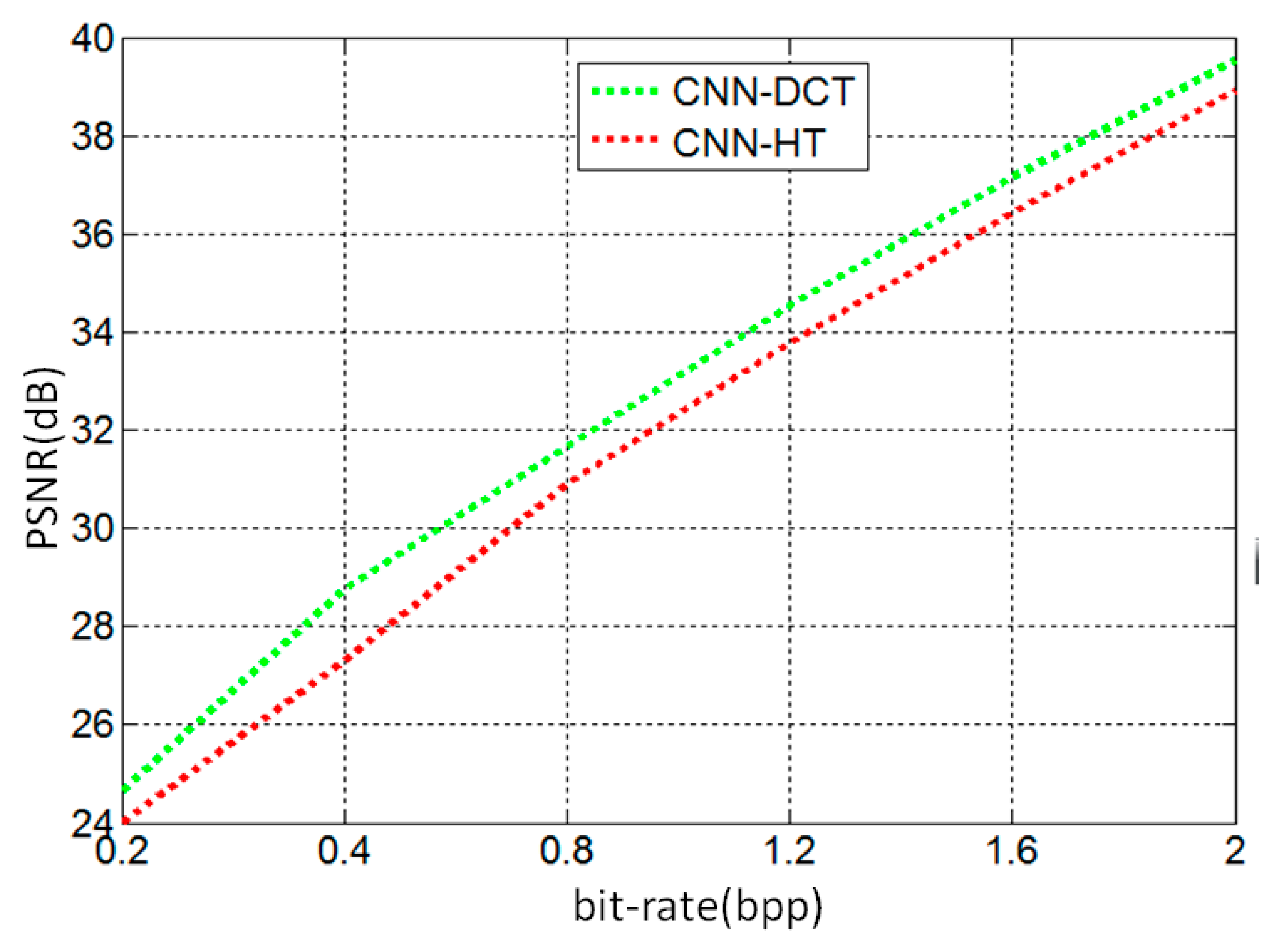
Hardmard Transform in CNNLower PSNR than DCT-CNNIn the convolution neural learning network, transform method is different from one used in compression link.

