Rebuilding a Microwave Soil Moisture Product Using Random Forest Adopting AMSR-E/AMSR2 Brightness Temperature and SMAP over the Qinghai–Tibet Plateau, China

Abstract

Time series of soil moisture (SM) data in the Qinghai–Tibet plateau (QTP) covering a period longer than one decade are important for understanding the dynamics of land surface–atmosphere feedbacks in the global climate system. However, most existing SM products have a relatively short time series or show low performance over the challenging terrain of the QTP. In order to improve the spaceborne monitoring in this area, this study presents a random forest (RF) method to rebuild a high-accuracy SM product over the QTP from 19 June 2002 to 31 March 2015 by adopting the advanced microwave scanning radiometer for earth observing system (AMSR-E), and the advanced microwave scanning radiometer 2 (AMSR2), and tracking brightness temperatures with latitude and longitude using the International Geosphere–Biospheres Programme (IGBP) classification data, the digital elevation model (DEM) and the day of the year (DOY) as spatial predictors. Brightness temperature products (from frequencies 10.7 GHz, 18.7 GHz and 36.5 GHz) of AMSR2 were used to train the random forest model on two years of Soil Moisture Active Passive (SMAP) SM data. The simulated SM values were compared with third year SMAP data and in situ stations. The results show that the RF model has high reliability as compared to SMAP, with a high correlation (R = 0.95) and low values of root mean square error (RMSE = 0.03 m³/m³) and mean absolute percent error (MAPE = 19%). Moreover, the random forest soil moisture (RFSM) results agree well with the data from five in situ networks, with mean values of R = 0.75, RMSE = 0.06 m³/m³, and bias = −0.03 m³/m³ over the whole year and R = 0.70, RMSE = 0.07 m³/m³, and bias = −0.05 m³/m³ during the unfrozen seasons. In order to test its performance throughout the whole region of QTP, the three-cornered hat (TCH) method based on removing common signals from observations and then calculating the uncertainties is applied. The results indicate that RFSM has the smallest relative error in 56% of the region, and it performs best relative to the Japan Aerospace Exploration Agency (JAXA), Global Land Data Assimilation System (GLDAS), and European Space Agency’s Climate Change Initiative (ESA CCI) project. The spatial distribution shows that RFSM has a similar spatial trend as GLDAS and ESA CCI, but RFSM exhibits a more distinct spatial distribution and responds to precipitation more effectively than GLDAS and ESA CCI. Moreover, a trend analysis shows that the temporal variation of RFSM agrees well with precipitation and LST (land surface temperature), with a dry trend in most regions of QTP and a wet trend in few north, southeast and southwest regions of QTP. In conclusion, a spatiotemporally continuous SM product with a high accuracy over the QTP was obtained.

1. Introduction

Soil moisture (SM) is a key state variable for understanding hydrological processes with a variety of environmental applications (e.g., ecological, geomorphological and water resource management) [1,2]. Soil moisture also plays an important role in the climate systems from local scales to global scales, and the Global Climate Observing System (GCOS) has deemed it as an essential climate variable (ECV) in 2010 [3].

The Qinghai–Tibet plateau (QTP) is also called the “water tower of Asia”. It is the headstream of seven major rivers in Asia. With an average altitude of more than 4000 m, the QTP has a great influence on the Asian monsoon and the global atmospheric cycle, and is a sensitive area to climate change. In other words, here global climate change can be effectively monitored. Obtaining a series of accurate soil moisture data in the QTP can provide important observations to understand the dynamics of land surface-atmosphere feedbacks in the global climate system [4]. However, observation data from long time series are very scarce and statements about the temporal variation of SM in the QTP remain vague. For example, long-term data products such as from the European Space Agency’s Climate Change Initiative (ESA CCI) [5], where different sensor types were merged by a cumulative distribution function (CDF)-matching procedure, temporal inconsistencies are introduced, e.g., due to different responses to the challenging terrain (e.g., from different microwave frequencies, active and passive operation modes etc.). Data assimilation products, such as from the Global Land Data Assimilation System (GLDAS) [6,7], usually present soil moisture data from deeper soil layers, which cannot respond to changes in the surface caused by some small precipitation events [8]. Additionally, the matching to the Noah model [9] makes it not an independent monitoring product. Low-frequency passive microwaves (such as the L-band) are less susceptible to vegetation and more sensitive to soil moisture. However, soil moisture and ocean salinity (SMOS) data from 16 January 2010 to the present [10] and soil moisture active passive (SMAP) data from 31 March 2015 to the present [11], which are based on L-band passive microwaves, have relatively short time series [12]. Previous studies [13,14,15,16,17] have shown that SMAP has a high accuracy both globally and over the QTP, but data from only three years (31 March 2015 to present) are available. Chen et al. [18] evaluated SMAP over the QTP and found good agreement according to the amplitude and temporal variation of the areal soil moisture, as indicated by small values of the unbiased root mean square error (ubRMSE) and high time series correlation coefficient (R), suggesting a satisfactory performance of the SMAP soil moisture product in the QTP. SMOS is heavily affected by radio frequency interferences (RFI) in this area, so that the number of valid soil moisture retrievals is limited. The advanced microwave scanning radiometer for earth observing system (AMSR-E), from June 2002 to October 2011, and the advanced microwave scanning radiometer 2 (AMSR2), from July 2012 to present have data from longer time series, and they have similar configurations and constitute a continuous time series. However, they significantly underestimate soil moisture and have a small variation range.

Therefore, high-accuracy and spatiotemporally continuous soil moisture products over the QTP for longer time periods are of great importance for monitoring the water and heat exchanges in this region and their impact on changing the water cycle and regional climate of East and Southeast Asia [19,20]. However, due to its topography, complex underlying surface and the effects of its freezing season, the QTP is a region where retrieving soil moisture is difficult. Although many studies have focused on merging multisource soil moisture products, the results obtained over the QTP usually have low performance or even lack values obtained over the whole QTP, especially in global products.

To solve this problem, multisource soil moisture products should be merged to take full advantage of the data from different sensors and to rebuild a longer time series data set. Zhang and Chen [21] presented a satellite and in situ sensor collaborated reconstruction (SICR) method adopting linear regression, the least square method, geostatistical interpolation algorithms, and similar pixel determination to reconstruct soil moisture data under full cloud contamination. Alyaari et al. [22] used simplified statistical regression by adopting SMOS SM and AMSR-E brightness temperatures (Tbs) to derive long-term global SM data sets with an average ubRMSE of 0.06 m³/m³. Another simple way to simulate SM is to train a machine learning model using Tbs and auxiliary data as input data and land surface parameters as output data. Rodriguez–Fernandez et al. [23] used a neural network (NN) to establish a model composed of L-band SMOS Tbs complemented with C-band advanced scatterometer (ASCAT) backscattering coefficients, as well as the moderate resolution imaging spectroradiometer (MODIS), the normalized difference vegetation index (NDVI), and a reference SM data set (European Centre For Medium-Range Weather Forecasts (ECMWF) model predictions). Cui et al. [24] used the back-propagation neural network (BPNN) adopting MODIS products (LST, NDVI, and albedo), other auxiliary data (longitude, latitude, digital elevation model (DEM), and day of the year (DOY)) and the FY (FengYun)-3B/MWRI (microwave radiation imager) SM product to rebuild SM on the QTP. The results show that the R² (coefficient of determination) is greater than 0.56, root mean square error (RMSE) is under 0.1 cm³/cm³, and bias is under 0.07 cm³/cm³. Yao et al. [25] also used the BPNN method to reconstruct a global SM data, adopting Tbs and MVI (microwave vegetation index) from AMSR-E/AMSR2 and SM from SMOS. The results agree well with network data, the R is 0.52, RMSE is 0.08 m³/m³ and bias is 0.002 m³/m³. Lu et al. [26] used a nonlinear autoregressive neural network (NARXnn) to retrieve SM in the Heihe River basin. They used daily Tbs, NDVI, precipitation, and DEM information as input data and the fused SM from the Japan Aerospace Exploration Agency (JAXA) and the land surface parameter model (LPRM) as output data. The results indicate that the retrieved SM has a good performance, with high correlation coefficient (R ≥ 0.85) and lower bias (−0.02 m³/m³ ≤ bias ≤ 0.02 m³/m³) and RMSE (RMSE ≤ 0.06 m³/m³).

Random forest (RF) is an ensemble classifier randomly selecting training samples and variables, and then generate many decision trees. This method has been used in remote sensing because of its high flexibility and precision [27]. RF is not easy to over-fit, and it has a very good anti-noise ability, extremely high accuracy and fast training speed, thus allowing it to process very high-dimensional data. It is widely used in classification [28,29] and prediction [30,31,32].

In this paper, we use the RF model to train AMSR-E/AMSR2 Tbs and auxiliary data (latitude, longitude, the International Geosphere-Biospheres Programme (IGBP), DEM and DOY) onto SMAP SM for the period of April 2015 to April 2017. The aim is to generate a consistent and high accuracy soil moisture time series from 2002 to 2015. This paper is organized as follows: in Section 2 the study area as well as the data set used in this paper are described. In Section 3, the description of the random forest method is provided, and the processing strategy used for random forest soil moisture (RFSM) generation is developed, including the training sample generation process and validation procedure. The validation results and trend analysis are shown in Section 4. Finally, Section 5 concludes the results.

2. Study Area and Data

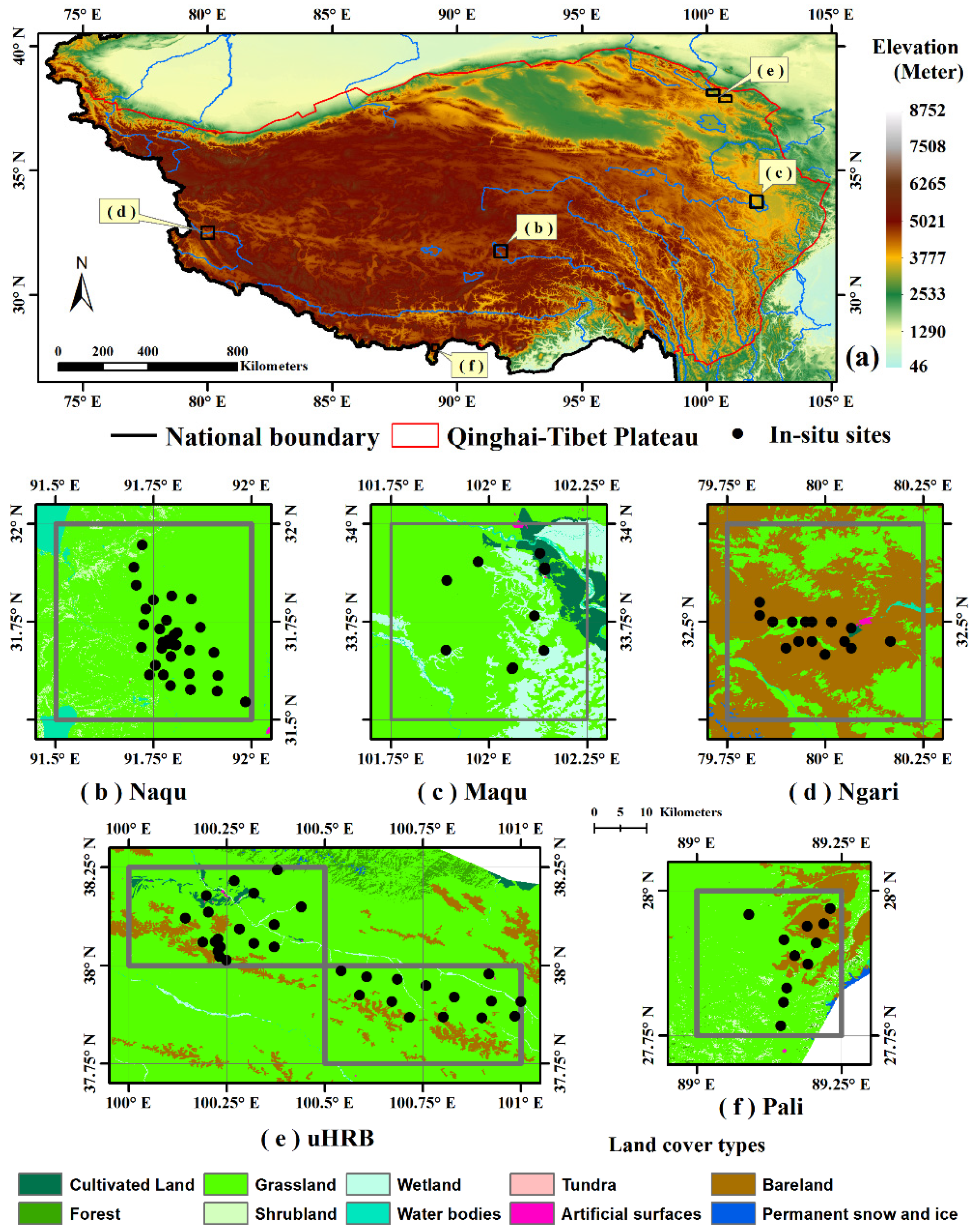
2.1. Study Area

The QTP is the highest mountain plateau in the world. It is also called “the third pole” or the “water tower of Asia”, and it is located between 26.5°–40°N and 73°–105°E (Figure 1). The QTP is approximately 2900 km long and 1500 km in wide, and the area is approximately 2.5 million km². Most of the QTP is located between 3000 and 5000 m above sea level, and the average elevation is above 4000 m. Surrounded by the earth’s highest mountains, the QTP is bordered by the Kunlun Range to the north, the Himalayan Mountains to the south, the Qilian Mountains to the northeast, and the Pamir and the Karakoram Range to the west; thus, it has long been known as the “roof of the world” [33]. A long time series climatic data record from 1961–2010 shows that the mean annual temperature is from −2.2 °C to 0 °C, the minimum value is −13.5 °C in January and the maximum value is 9.7 °C in July. The mean annual sunshine duration is from 2730 h to 2915 h, the average annual potential evapotranspiration is about 940 mm [34]. The mean annual precipitation is between 415 mm and 512 mm, and 73% of the precipitation occurs in summer and autumn.

The QTP also has a broad variety of ecosystem types, ranging from desert in the northwest to forests in the southeast. The major land cover types in QTP include grasslands, shrublands, forest, bare land and glaciers, and croplands. The grassland accounts for more than 55% of the total area, which is the major land cover in QTP [35].

2.2. In Situ Network Data

In this paper, five soil moisture ground measurement networks are used, namely, the Naqu network, the Maqu network, the Ngari network, the upper reach of the Heihe River Basin (uHRB) network, and the Pali network. The DEM (GTOPO-30, https://lta.cr.usgs.gov/GTOPO30.org/) and land cover map (GlobeLand30-2010, http://www.globeland30.org/) of each network are shown in Figure 1.

The Naqu network is located in the central QTP, at approximately 31°–32°N and 91.6°–92.5°E, and it has a cold, semi-humid climate. A dense monitoring network has been established at three spatial scales (1.0, 0.3, and 0.1 degrees) to measure temperature and soil moisture of 0–~5, 10, 20 and 40 cm in depth [36]. The mean value of the 31 sites in the gray box, which contains four 0.25° pixels, was calculated.

The Maqu network is located in the east of the QTP, at approximately 33.5°–34.25°N and 101.75°–102.75°E, and it has a humid climate. Temperature and soil moisture data at a depth of 5 cm were monitored in 15 min intervals from 13 May 2008 to 20 May 2016. Eight sites in the four 0.25° pixels in the gray box were used to calculate the mean value.

The Ngari network is located in the western region of the QTP, at approximately 79.75°–80.25°N, 79.5°–79.75°E [37]. Its climate is arid, and most of the region is covered by bare land and grassland. Temperature and soil moisture data were recorded from 22 July 2010 to 13 August 2016 in 15 min intervals. The mean value was calculated from fifteen sites in Ngari.

The uHRB network is located in the northeast of QTP, at approximately 37.75°–38.5°N and 100°–101.25°E, and it includes 40 WATERNET sites that were optimally laid out [38] on the upper reaches of the Heihe River basin during the HiWATER experiment [39,40,41,42,43]. Soil moisture and temperature data were monitored at 4, 10, and 20 cm in depth from 1 July 2013 to 31 December 2015. The mean value of the forty sites in the two gray boxes in Figure 1, which contain four 0.25° pixels, were calculated and used as in situ data.

The Pali network locates in the north of QTP, at approximately 27.75°–28°N and 89°–89.25°E. There are 25 sites in this network, and it has a semi-arid climate. Temperature and soil moisture data were recorded at depths of 5, 10, 20 and 40 cm from 21 June 2015 to 27 September 2016 in 0.5-h intervals. In addition, 11 sites in the gray box in Figure 1 were used in this work, and the mean value of these 11 sites was used as reference data.

2.3. Data Sets for Random Forest

2.3.1. Brightness Temperature and Soil Moisture of AMSR-E/AMSR2

AMSR-E is the first satellite sensor used for SM monitoring expecting error levels less than 0.06 m³/m³ [44]. AMSR-E is a passive microwave radiometer with multifrequency capabilities aiming to detect microwave emissions from land surface and atmosphere. Its time of ascending was 13:30 (local time) and its time of descending was 01:30 (local time), and its duration extended from June 2002 to October 2011. Double polarization brightness temperatures are measured at six frequencies (6.9 GHz, 10.7 GHz, 18.7 GHz, 23.8 GHz, 36.5 GHz, and 89.0 GHz), with an incidence angle of 55°.

AMSR2 was carried by the Global Change Observation Mission-W1 (GCOM-W1) satellite and successfully launched by JAXA in May 2012. It has provided observational data since 3 July 2012. AMSR2 is a continuation of AMSR-E, and it has the same ascending and descending times as AMSR-E. Compared with AMSR-E, it contains a newly added 7.3 GHz channel at C-band, and its overall reliability has thus been improved to a certain extent.

AMSR-E L3 Tb data has a spatial resolution of 25 km with equal-area scalable earth (EASE)-grid projection (global cylindrical). The AMSR2 L3 Tb has a resolution of 0.25°, with an equi-rectangular (EQR) projection. Both AMSR-E and AMSR2 are used to generate two SM product lines. One is produced by JAXA (Japan Aerospace Exploration Agency) and it is derived from a look-up table. The other product is generated by the Free University of Amsterdam with the National Aeronautics and Space Administration (NASA) using the land parameter retrieval model (LPRM) method.

In this paper, five descending Tb products (level 3, double polarization of 10.7 GHz and 18.7 GHz, V polarization of 36.5 GHz) of AMSR2 from April 2015 to April 2017 were used to train the random forest model. Tbs data from 19 June 2002 to 3 October 2011 from AMSR-E and those from 3 July 2012 to 31 March 2015 from AMSR2 were used to rebuild a longer time series of SM data. In addition, two SM products (Level 3, JAXA and LPRM) were used to compare the newly rebuilt SM products obtained from the random forest model based on SMAP SM, AMSR2 Tbs and other predictors.

The Tb products and the JAXA SM products can be downloaded from the Globe Portal Svstem (G-Portal), http://gportal.jaxa.jp/gpr/, and the LPRM SM product can be downloaded from Goddard Earth Sciences Data and Information Services Center (GES DISC), http://disc.gsfc.nasa.gov/hydrology/data-holdings.

2.3.2. The SMAP Soil Moisture Product

NASA’s SMAP satellite was launched on 31 January 2015. Its payload sensor uses the L-band microwave frequency, which is most suitable for SM retrieval. The revisit interval of SMAP is 2–3 days, thus allowing it to be used for the rapid monitoring of global SM [45]. Its ascending time is 6:00 pm (local time), and its descending time is 6:00 am (local time). The active radar and radiometer of the L band work together to measure SM and freeze-thaw state data. However, the L-band active radar only produced data for 11 weeks before it stopped operation on 7 July 2015.

Previous studies have shown that the temperature in the morning is more uniform than that at night, which is more conducive to SM retrieval. Therefore, the precision of the SMAP descending SM product is higher than that of the ascending product [46]. For this reason, the SMAP L3 descending SM data were used in this work; the product has a resolution of 36 km. The SMAP L3 daily SM products [47] are freely available on the National Snow and Ice Data Center (NSIDC), at http://nsidc.org/data/smap/.

This paper used three years’ worth of SMAP L3 SM products. The data from April 2015 to April 2017 (two years) were used to train the Tbs of AMSR-E/AMSR2 and auxiliary data to establish a random forest model, and the data from April 2017 to April 2018 (one year) were used to test the model.

2.3.3. Other Auxiliary Data Used as Spatial Predictors

The global 30-arc second elevation dataset (GTOPO-30) is a global DEM covering all regions from 180°W to 180°E and from 90°S to 90°N. It has a resolution of 30 s. This data set was developed by the United States Geological Survey (USGS). The elevation reference of GTOPO-30 is the mean sea level, and the horizontal coordinate system is world geodetic system 1984 (WGS 84). Here, the GTOPO-30 data were resampled to a resolution of 0.25°. The GTOPO-30 data can be obtained from the USGS (https://lta.cr.usgs.gov/GTOPO30).

MCD12Q1 land cover data are based on one year of Terra and Aqua observation data. In this paper, the land cover classification system of the IGBP was used. According to the IGBP, the land cover data set contains 17 main types of land cover, including 11 natural vegetation types, three land development and inlaid land categories and three non-grass land types.

Another MODIS data used in this paper was MOD11C3 monthly land surface temperature (LST) with a resolution of 0.05°. The LST is used to evaluate the temporal trend performance of RFSM. The MCD12Q1 and MOD11C3 product can be downloaded from the EARTHDATA website (https://search.earthdata.nasa.gov/).

In addition, precipitation data used in this paper were extracted from the gridded daily scale data set of CN05.1 [48], which is an augmentation of CN05 [49], is based on the interpolation of more station observations (~2400) and is characterized by a higher spatial resolution of 0.25° × 0.25°.

2.4. ESA CCI Soil Moisture Product

The Soil Moisture Climate Change Initiative (CCI) project is an important part of the European Space Agency (ESA) program on the Global Monitoring of Essential Climate Variables (ECVs). This project aims to produce consistent global SM data set based on active and passive microwave sensors [50].

The ESA CCI SM has three data sets, namely, active, passive and combined data. In this work, the passive data set (v03.2) was used to be compared with the RFSM. The dual-channel Land Parameter Retrieval Model version 3 (LPRM v3; [51]) was used to convert the Tbs data into SM values.

The grid of the passive data set products is 0.25° × 0.25° based on WGS 84 reference system. Its dimension is 1440 × 720. These products are available from the ESA CCI (https://www.esa-soilmoisture-cci.org/).

2.5. GLDAS Soil Moisture Product

The GLDAS was developed by both NASA’s Goddard Space Flight Center (CSFC) and the National Oceanic and Atmospheric Administration (NOAA) national centers for environmental prediction (NCEP) [52]. It is an offline terrestrial modeling system providing optimal simulations of the global land surface states and fluxes. These data are also available on the GES DISC (http://disc.gsfc.nasa.gov/hydrology/data-holdings).

In this paper, the GLDAS-2.1 Noah Land Surface Model L4 data with a temporal resolution of three hours and a spatial resolution of 0.25° was used as the reference SM. The GLDAS-2.1 data are archived and distributed in NetCDF format. To match the descending time of the SMAP SM data, only the 06:00 values were used.

3. Methodology

Random forest is a classifier that uses multiple classification and regression trees (CARTs), where each tree is not related to another, to train samples and then to classify new input samples or to predict values. The two most important parameters of random forest are the number of trees (ntree) and the number of features (mtry). In random forest samples, the input data is organized in rows (samples) and columns (features). For row sampling, the strategy is to perform replacement sampling, which means that some samples may appear several times in the training set of a tree or may never appear. In this way, during training, the input samples of each tree are not the total samples, which makes it relatively unlikely to over-fit. Then, column sampling is performed (i.e., each sample is classified based on the feature variable), and m features are selected from the entire set of M features (m < M). Subsequently, the decision tree is established by using the complete split method on the sampled data. After obtaining the forest, let each decision tree in the forest judge and regress separately when a new input sample is entered. Then, take the average value of all trees as the final result. An important advantage of random forest is that it is not necessary to cross-verify or to obtain an unbiased estimate of the error with an independent test set. The error can be evaluated internally, i.e., an unbiased estimate of the error can be established during the process of generation. For each tree (suppose for the k tree), approximately a third of the training samples are not involved in the generation of the k tree, which is called the out-of-bag (oob) sample of the k tree. After the random forest model is constructed, these samples are classified, and the ratio of the number of misdivisions to the total number of samples is used as the oob misclassification rate of the random forest.

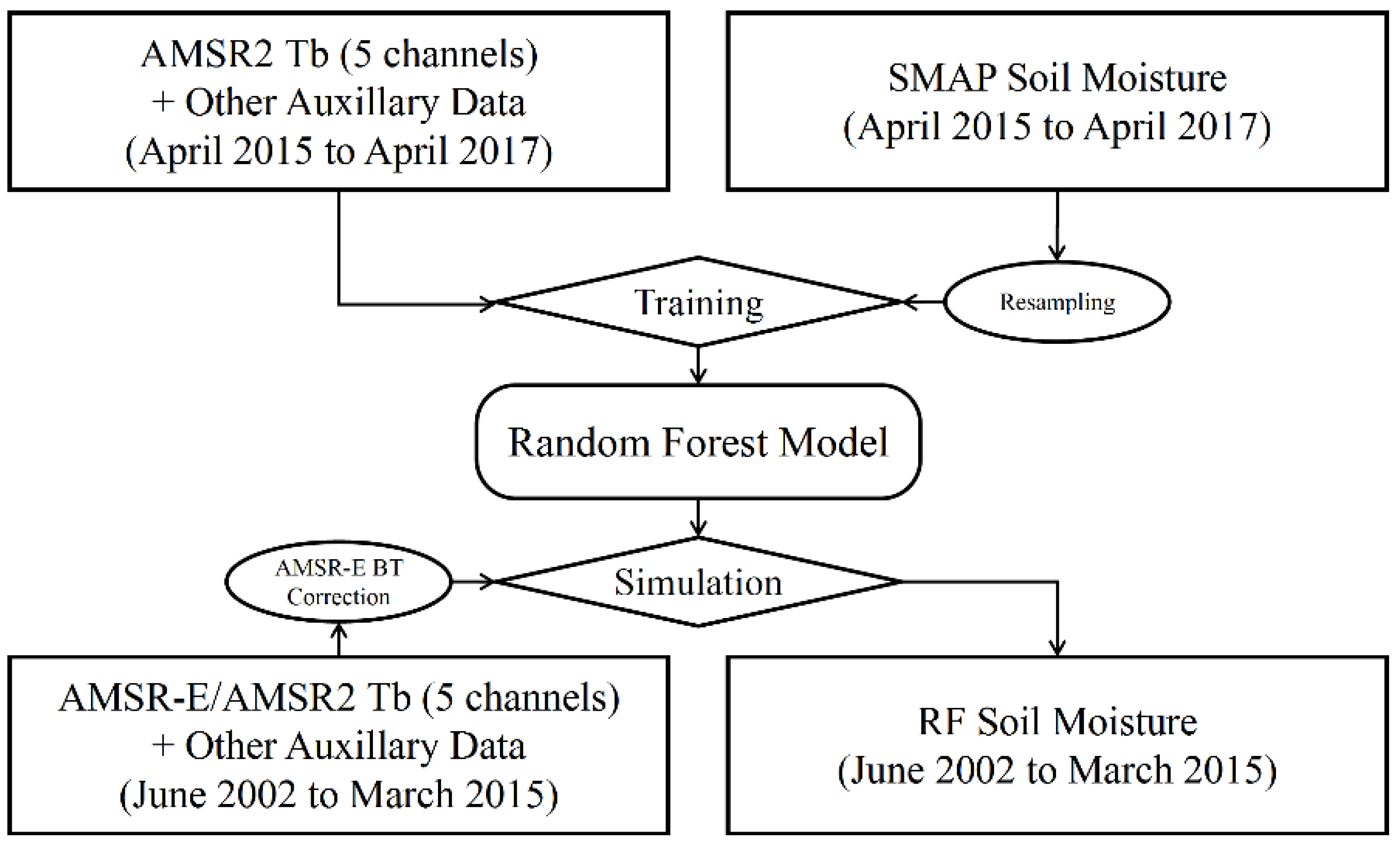
3.1. Processing Strategy for Random Forest SM Generation

To build the random forest model, 10 input features and one output feature were used. The input features include: 5 Tb products (double polarization of 10.7 GHz and 18.7 GHz, V polarization of 36.5 GHz), DEM (GTOPO-30), IGBP (IGBP global vegetation classification), latitude, longitude, and DOY. The flow chart is shown in Figure 2.

It is worth noting that there is a correction process for AMSR-E Tbs in the flow chart (Figure 2). The reason for this is that although the AMSR-E and AMSR2 sensors are similar, there are still differences in the observed Tbs data caused by their different calibration procedures and sensor specifications [53]. This requires the calibration of the two sensors so that their observations can maintain a high consistency.

There are three methods to intercalibrate sensors [54]: (1) the simultaneous nadir overpass (SNO) approach; (2) statistical intercalibration; and (3) double differencing (DD) methods. In this paper, the correction results [55] shown in

Table 1. Brightness temperature biases correction of advanced microwave scanning radiometer for earth observing system (AMSR-E) to the advanced microwave scanning radiometer 2 (AMSR2).

Pairwise Comparisons	bias
	H_Pol	V_Pol
10 GHz
MWRI-AMSR-E	−1.39	−2.23
MWRI-AMSR2	−4.04	−4.43
AMSR2-AMSR-E	2.65	2.11
18 GHz
MWRI-AMSR-E	0.84	1.07
MWRI-AMSR2	−0.93	−1.07
AMSR2-AMSR-E	1.77	2.14
36 GHz
MWRI-AMSR-E	-	−2.84
MWRI-AMSR2	-	−3.94
AMSR2-AMSR-E	-	1.1

were used. The DD method was applied in this paper using an intermediate reference (MWRI) which both sensors have to quantify the Tbs differences between the AMSR-E and AMSR2 Tbs data, because the integrated multisensor Tbs record was largely consistent over most global regions. After the correction of biases, the AMSR-E Tb can be used as AMSR2 Tb in the RF model.

Land cover types play an important role in the retrieval of SM; land cover data used here is the IGBP global vegetation classification data from MCD12Q1. To simplify the model, the land cover types used in this paper are divided into four categories based on their IGBP classifications, namely, barren or sparsely vegetated, grasslands and shrublands, forests, and water and ice/snow cover. In this paper, ice/snow cover data are not used to build the random forest model, and SM is not simulated over ice/snow cover. The details are shown in

Table 2. Classification used in random forest (RF)-based on International Geosphere-Biospheres Programme (IGBP) global vegetation classification.

The Classification Used in RFSM	IGBP Global Vegetation Classification from MCD12Q1	IGBP Class Number
Barren or Sparsely Vegetated	Barren or Sparsely Vegetated	16
Grasslands and Shrublands	Closed Shrubland	6
	Open Shrublands	7
	Grasslands	10
	Crop	12
Forests	Evergreen Needleleaf Forest	1
	Evergreen Broadleaf Forest	2
	Deciduous Needleleaf Forest	3
	Deciduous Broadleaf Forest	4
	Mixed Forests	5
Water and ice/snow cover	Water	0
	Snow and Ice	15

.

In this article, the two-year data (April 2015 to April 2017) for each pixel were used to train the model. To keep the orders of magnitude consistent between variables, including the input and output variables, each variable was normalized to 0–1. After this simulation, the output variable was reversely normalized to obtain the RFSM value.

3.2. Validation and Trend Analysis Procedure

The RFSM product needed to be tested before it can be applied. To test the training result, it was necessary to compare the RFSM with the SMAP SM to test the prediction accuracy. Therefore, we compared the RFSM values with the data obtained from the five in situ SM networks. As mentioned in Section 2.2, we used the mean values of all sites located in the gray box in Figure 1 as the in situ values. This evaluation was performed using the correlation coefficient (R), root mean square error (RMSE), mean absolute percentage error (MAPE) and bias values, which are defined as follows:

$$R=\frac{\sum \left(x_i-\overline{x}\right)\left(y_i-\overline{y}\right)}{\sqrt{\sum {\left(x_i-\overline{x}\right)}^2\sum {\left(y_i-\overline{y}\right)}^2}}$$

(1)

where $\overline{x}$ and $\overline{y}$ indicate the mean values, $x_i$ is the RFSM value, and $y_i$ is the SMAP SM or in situ SM observation value.

$$\mathrm{RMSE}=\sqrt{\frac{\sum {\left(x_i-y_i\right)}^2}{N}}$$

(2)

$$\mathrm{MAPE}=\frac{1}{N}·\sum \left|\frac{x_i-y_i}{y_i}\right|·100$$

(3)

$$\mathrm{bias}=\frac{1}{N}\sum \left(x_i-y_i\right)$$

(4)

where N is the number of matching data points.

However, the available quantity of in situ data is usually not sufficient, and these data thus cannot reflect the precision of the product over the entire region. The three-cornered hat (TCH) is an alternative method which can calculate the uncertainty of each product in each pixel over the study area.

The TCH method is based on removing common signals from observations and then calculating the uncertainties which can reflect their measurement errors [56]. Chin et al. [57] indicated that this method is simple to achieve, but needs at least three data sets that are statistically independent. This method has been used in geodesy and hydrology before [58]. A normal distribution of the observational errors and the theory is assumed, and described as follows:

$$ob{s}_i=x+e_i$$

(5)

where $ob{s}_i$ indicates observations, $x$ is the true value, and $e_i$ is the associated measurement error. Given three pairs of observations (i, j, k), the difference between observations (i, j) can be written as:

$$ob{s}_i-ob{s}_j=x+e_i-\left(x+e_j\right)=e_i-e_j$$

(6)

The associated variance can be described as:

$${\sigma }_{ij}^2={\sigma }_{ei}^2+{\sigma }_{ej}^2-2·cov\left(e_i,e_j\right)$$

(7)

We assumed the data sets are statistically independent, so that $cov\left(e_i,e_j\right)$ equals zero. Finally, the individual variances may be separated by:

$${\sigma }_{ei}^2=\frac{1}{2}·\left({\sigma }_{ij}^2+{\sigma }_{ik}^2-{\sigma }_{jk}^2\right)$$

(8)

If the results were negative, the absolute value was taken, and then the standard deviation is used as the uncertainty measure.

Mann–Kendall is a nonparametric test method. It does not require samples to follow a certain distribution, is not affected by anomaly data, and is suitable for sequential data. The Mann–Kendall test has been successfully applied in hydrology and meteorology [59,60] to analyze trends in time series. When using the Mann–Kendall method for trend analysis, the x value is regarded as a set of independently distributed sample data, and the parameter $Z$ is used as the pixel attenuation index. The calculation formula is as follows:

$$Z\{\begin{array}{c}\frac{S-1}{\sqrt{VAR\left(S\right)}} ,\hspace{1em}S>0\\ 0 ,\hspace{1em}\hspace{1em} S=0\\ \frac{S+1}{\sqrt{VAR\left(S\right)}} ,\hspace{1em}S<0\end{array}$$

(9)

where, the $S$ is the cumulative number of $x_i$ greater than or less than $x_j$ and $VAR\left(S\right)$ is the variance of $S$. They can be calculated as:

$$S={\displaystyle \sum }_{i=1}^{n-1}{\displaystyle \sum }_{j=i+1}^{n}sgn\left(x_j-x_i\right)$$

(10)

$$sgn\left(x_j-x_i\right)=\{\begin{array}{c} 1 ,\hspace{1em}{x}_j-x_i>0\\ 0 ,\hspace{1em}{x}_j-x_i=0\\ -1 ,\hspace{1em}{x}_j-x_i<0\end{array}$$

(11)

$$VAR\left(S\right)=\frac{n\left(n-1\right)\left(2n+5\right)}{18}$$

(12)

where n is the number of data in the sequence. $Z$ value is used to determine the significance level. At a given significance level, here α = 0.05, the threshold of the normal distribution is $Z_{1-a/2}$. When $\left|Z\right|\le Z_{1-a/2}$, the trend is insignificant, and when $\left|Z\right|>Z_{1-a/2}$, the trend is significant.

4. Results and Discussion

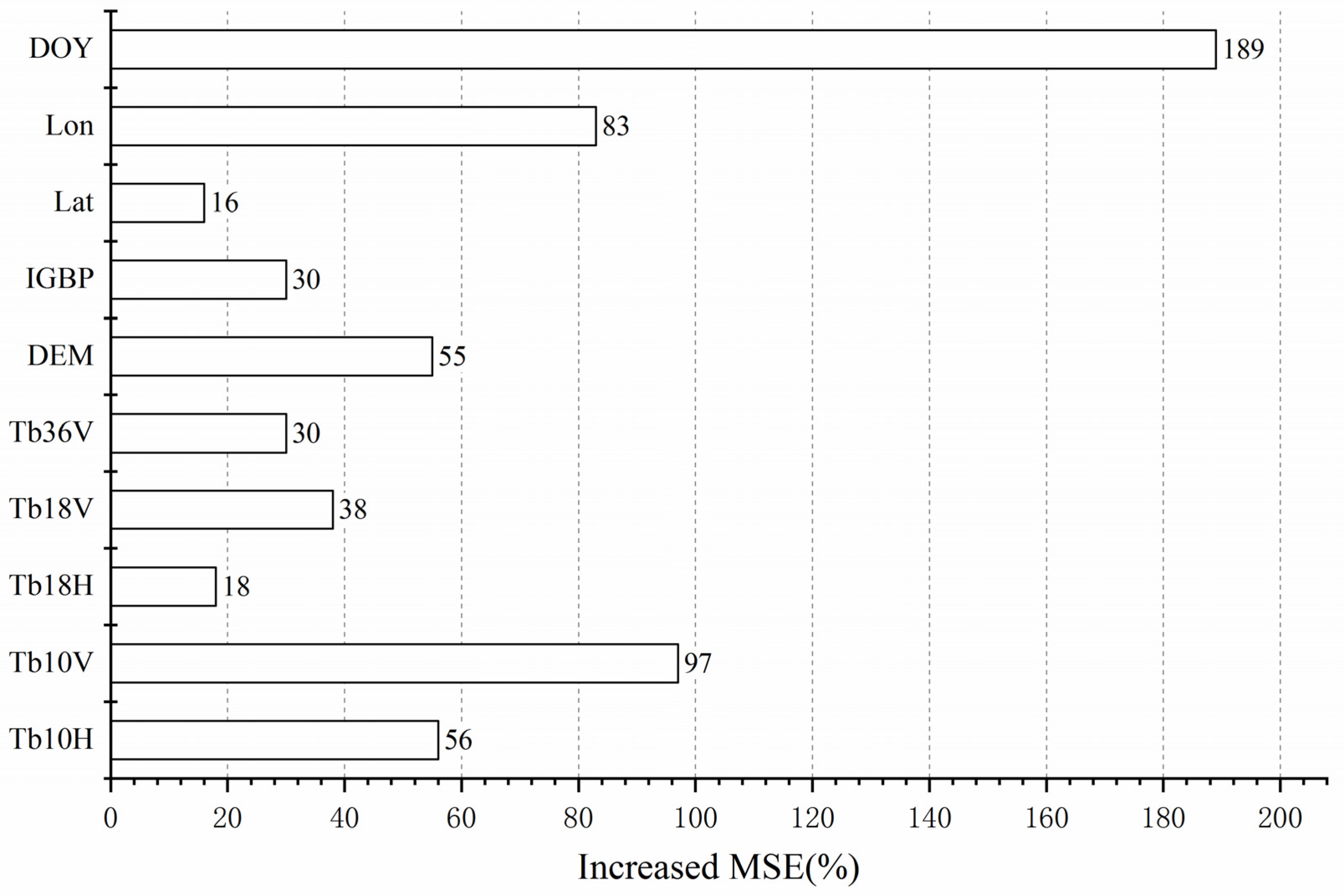
4.1. Variable Importance in Random Forest Model

RF can indicate the relative importance of a variable as an increased mean square error (MSE) [61]. An increased MSE can be calculated by randomly assigning a variable to compute the extent of the reduction in the accuracy of the random forest prediction. The larger this value, the greater the importance of the variable. The results shown in Figure 3 indicate that the most important five variables were DOY, Tb10V, longitude, Tb10H and DEM. As the time series in Section 4.3.1 shows, the SM data on the QTP have very similar seasonal variation; in most areas, the amount of rainfall was not high, thus making DOY a very important variable. The Tb of 10 GHz was used to retrieve SM in the JAXA and LPRM SM products, and it was very sensitive to SM.

As shown in the topography in Figure 1, the elevation of the west QTP was higher than that of the east QTP, with large variations in the longitudinal direction and small variations in the latitudinal direction. The distribution of SM is affected by DEM because the DEM indirectly affects vegetation, precipitation and other factors that are very sensitive to SM [62]. Interestingly, latitude usually represents the energy distribution, which is important to the SM distribution. However, the results in Figure 3 show that longitude was a more important factor than latitude in the random forest model because, as mentioned above, the altitude of QTP is high in the West and low in the East, so changes in the latitudinal direction are not obvious, and the longitude also reflects the DEM information. In addition, during the summer, the southwest monsoon from the Indian Ocean is blocked by the Himalayas, leading to relative drought in the southwestern part of the QTP, which makes the variation in SM on the QTP smaller in the latitudinal direction than in the longitudinal direction.

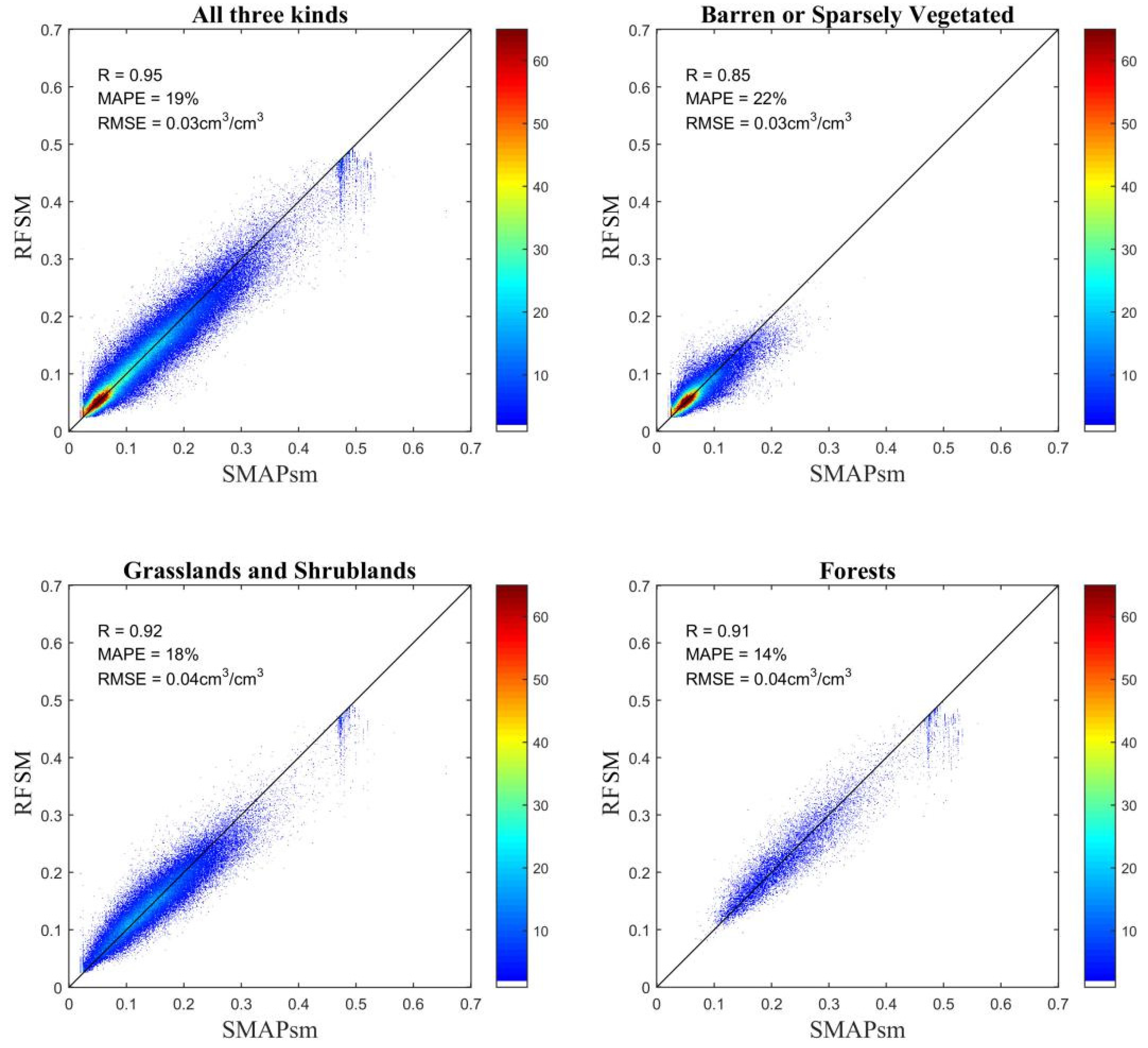
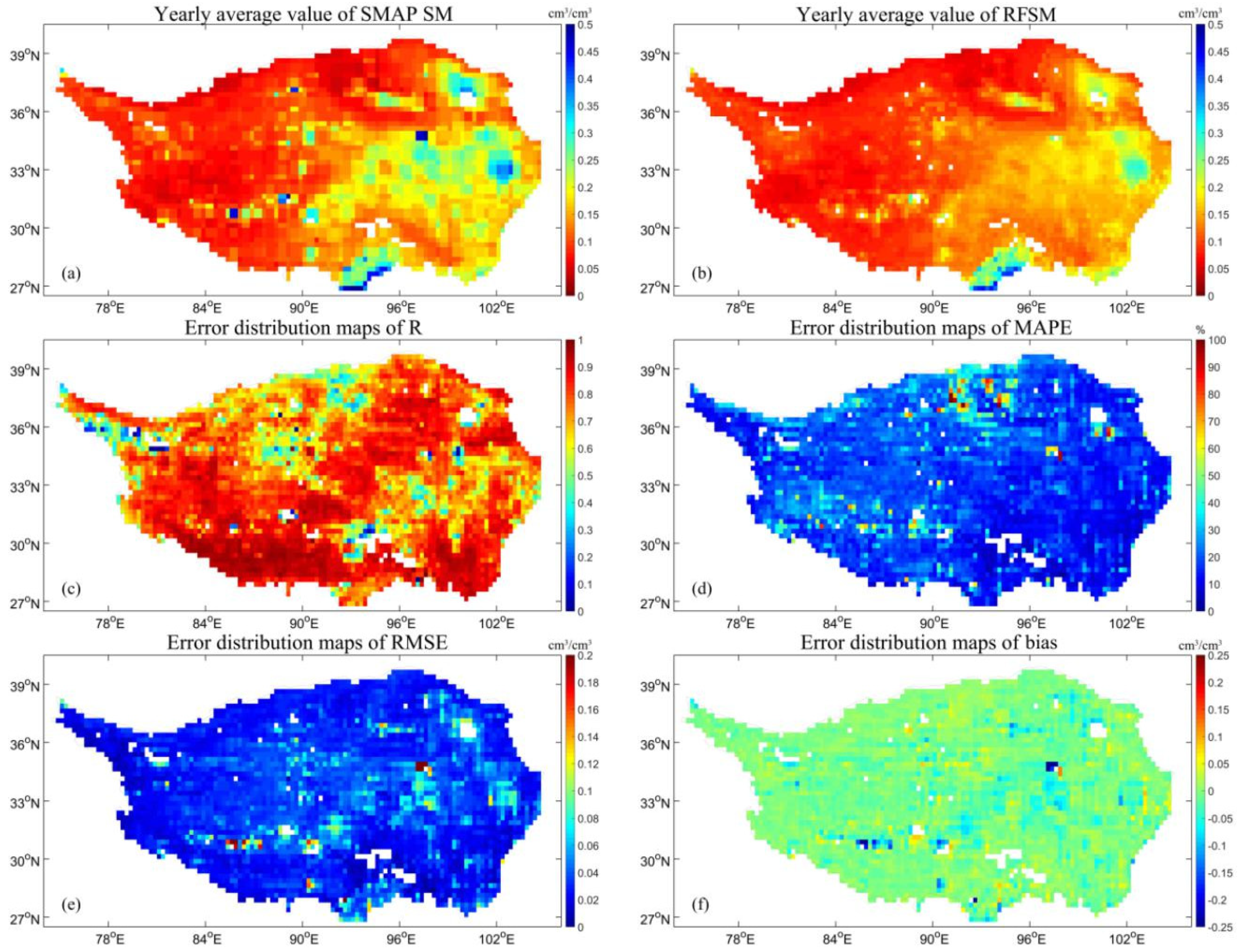
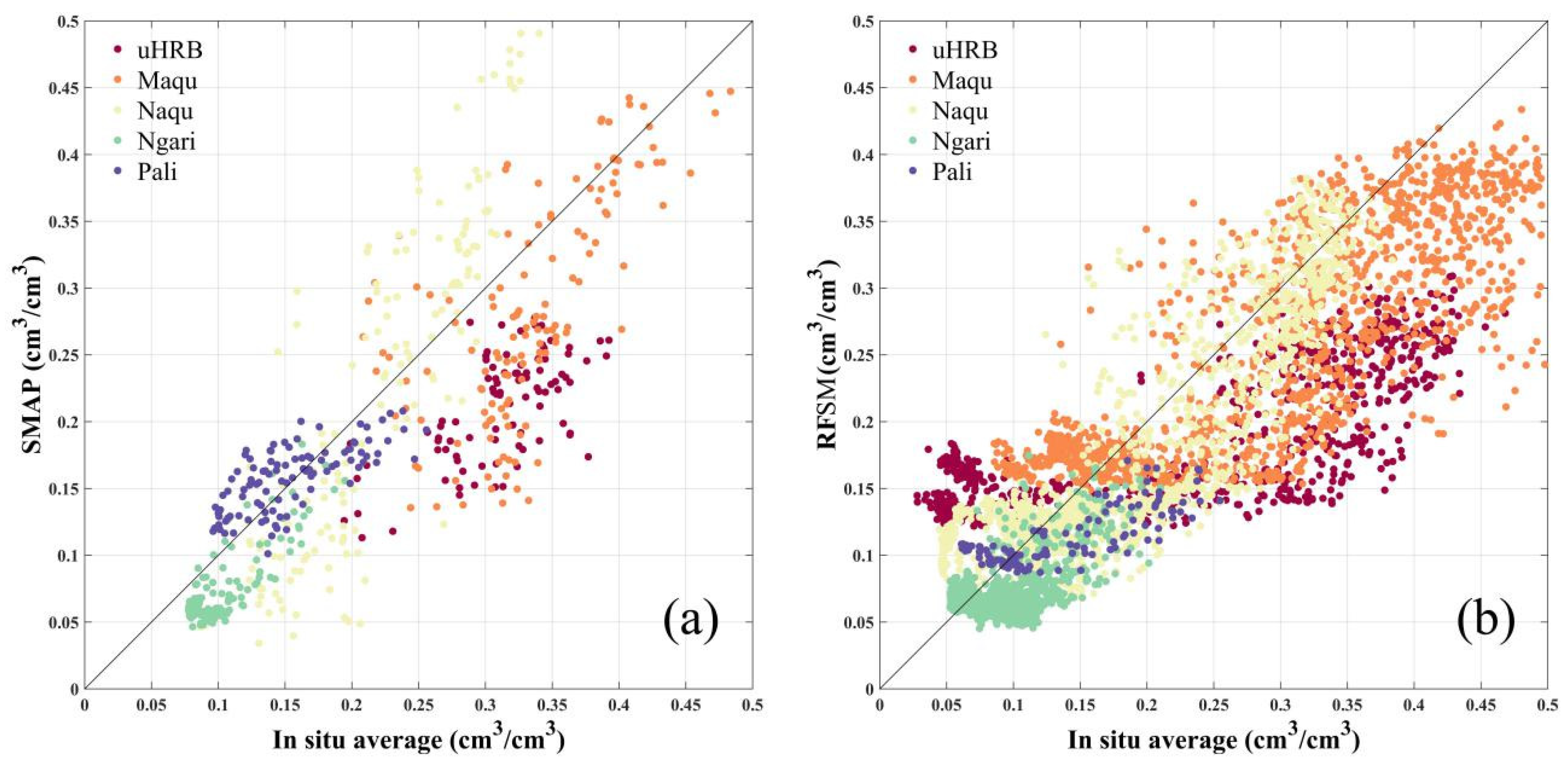
4.2. Comparison of RFSM and SMAP

We evaluated the quality of the RF simulation results by analyzing the agreement between RFSM and SMAP SM over the test period (May 2017 to May 2018) in terms of their R, MAPE, RMSE and bias values. In addition, the density scatterplots based on different land cover types are shown in Figure 4. The yearly mean values of SM and their error distribution maps are shown in Figure 5.

In Figure 4, the total accuracy and the accuracies obtained in barren or sparsely vegetated land, grasslands and shrublands, and forests are shown. In general, most of the points were located near the 1:1 line, with high R values (R = 0.95) and low values of RMSE (RMSE = 0.03 m³/m³) and MAPE (MAPE = 19%). Among the three land cover types, barren or sparsely vegetated land has a relatively poor accuracy (R = 0.85 and MAPE = 22%), which is partly because the emissions from bare land are significantly affected by surface roughness, which decreases the sensitivity of Tbs to SM [63,64,65]. Although roughness is addressed in the retrieval algorithm of SMAP, AMSR2 Tbs data are not calibrated for roughness. Therefore, the correlation between AMSR2 Tbs and SMAP SM was relatively poor in barren or sparsely vegetated regions, but it is still acceptable. Moreover, as the dynamic range of SM is small in desert or barren land, the correlation can become distorted by noise. However, in contrast to barren or sparsely vegetated land, the accuracy in grasslands and shrublands and forests was relatively good.

As shown in Figure 4, SMAP has a range of between 0.02 and 0.5, and the range of RFsm is between 0.02 and 0.5 as well. While the RFSM values are partly overestimated around 0.02 and underestimated around 0.5 because AMSR2 Tbs and SMAP SM do not have a strictly linear relationship, that is, some of the SM values around 0.02 or 0.5 match up with a wider range of Tbs values, and these Tbs values may also correspond to higher or lower values of SM on other trees in the RF model. In addition, random forest cannot make predictions beyond the input range (SMAP minimum and maximum values are 0.02 and 0.5, respectively). This means that no values lower than 0.02 and higher than 0.5 can be predicted. Because the final prediction of random forest involves the average values of multiple trees, this averaging process resulted in an overestimate or underestimate around 0.02 or 0.5, respectively. For values between 0.02 and 0.5, the overestimation and undervaluation can be partly offset by averaging multiple trees. Therefore, no obvious overestimation or undervaluation occurred in the range of 0.02–0.5.

In Figure 5, the yearly average values of SMAP SM and RFSM are shown, and the errors of RFSM vs. SMAP SM are calculated in terms of their R, MAPE, RMSE and bias values. Figure 5a,b show that SMAP SM and RFSM have very similar spatial distributions, in which the Chaidamu Basin can be clearly distinguished in the Northwest, Qinghai Lake is in the Northeast, high-value forest areas are in the South and grassland that is often flooded in the East. However, there is a certain degree of smoothness, especially over grasslands. This is affected by the classification error and the fact that the final prediction of the random forest model is taken from the average values of multiple trees. In Figure 5c, we can see that the accuracy of RFSM was very good, with a mean value of R = 0.79; in most regions, the R value was relatively high (R > 0.85), and most of the low values are distributed in the Northwestern and Eastern regions of the QTP. The land cover of the Northwestern QTP is barren land, with ice and snow cover located in the West, where the R values are low (R < 0.6). As shown in Figure 4, the RFSM accuracy in barren or sparsely vegetated land (R = 0.85) was not as good as that observed in the other two land cover types; in addition, it was also affected by ice and snow cover, which may not be reflected in the IGBP resampling process. The other low R values located in the East are affected by the smoothing effect, as shown in Figure 5a,b. The distribution of MAPE is shown in Figure 5d; it had a mean value of 17%, which is acceptable, with high values occurring in the regions of barren land where the correlation between AMSR2 Tbs and SMAP SM is not very strong, or near waterbodies due to the classification error (waterbodies to grasslands). In Figure 5e, the RMSE distribution map is plotted; it has a mean value of 0.03 m³/m³, and low values of ~0.02 m³/m³ occurred in most regions on the QTP. This indicates that the RF simulated result is relatively stable compared to SMAP SM. High RMSE values are caused by the smoothing effect and the incorrect classification of waterbodies and grasslands. Figure 5f shows the distribution of bias, which had a mean value of −0.01 m³/m³ and exhibited high values emerging near waterbodies, similar to the MAPE and RMSE data. This result shows that the RFSM was almost unbiased compared to SMAP SM. All four parameters show that RFSM is very stable, unbiased and relatively similar to SMAP SM, thus indicating that the RF model can be used to simulate SM data with high accuracy.

4.3. Evaluation of RFSM

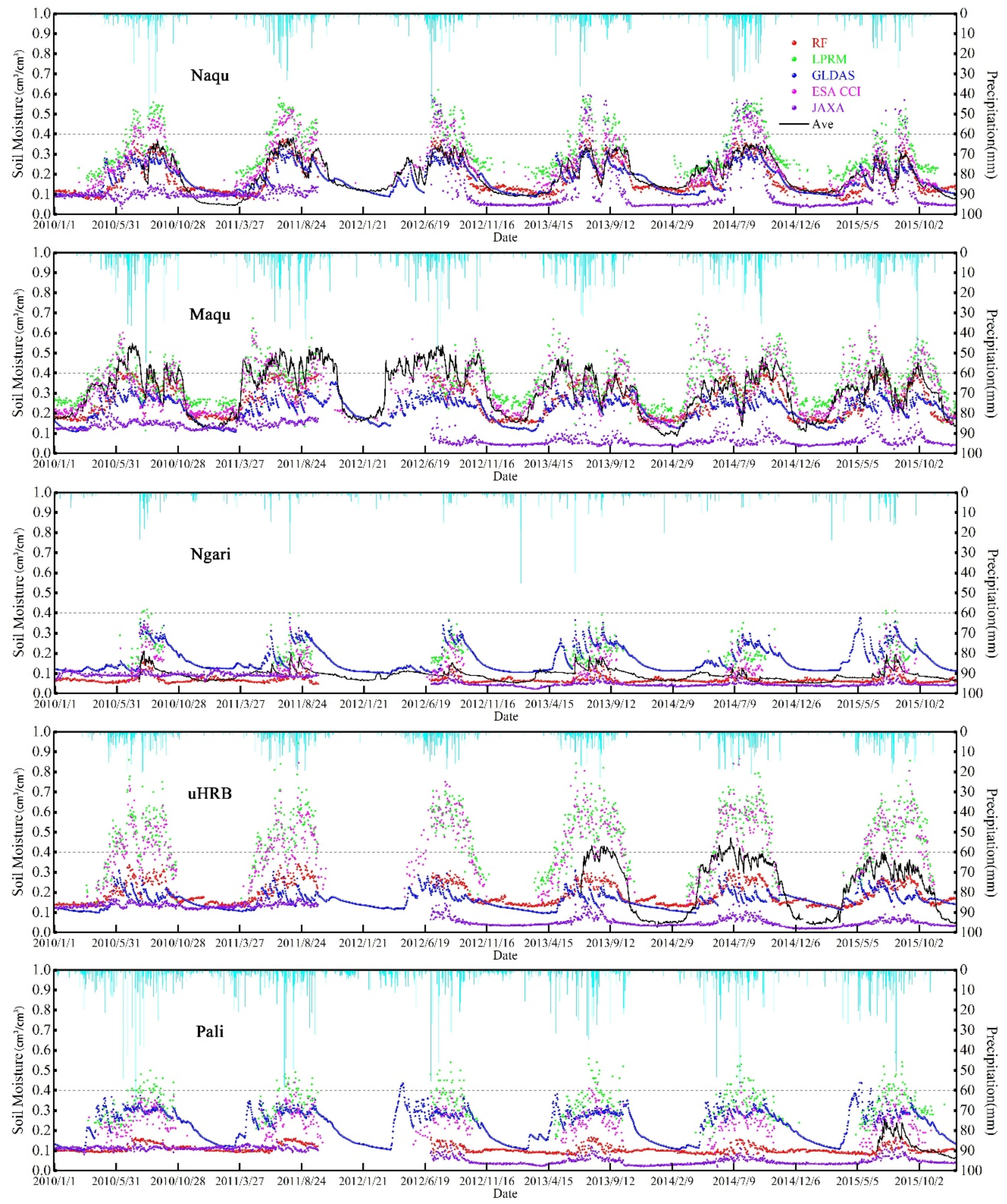
4.3.1. Comparison Against In Situ Data

To further evaluate the performance of RFSM over time, the validation results of SMAP SM over the period from 1 April 2015 to 31 December 2016 is listed in

Table 3. The performance metrics for soil moisture active passive (SMAP) soil moisture (SM) data over the five networks, during 1 April 2015 to 31 December 2016. The value N indicates the number of data can be used to validate SMAP over five networks.

In Situ Network	The Whole Year				Unfrozen Seasons
	RMSE	R	Bias	N	RMSE	R	Bias	N
Naqu network	0.076	0.867	0.008	152	0.076	0.861	0.011	148
Maqu network	0.079	0.691	−0.051	134	0.063	0.710	−0.032	100
Ngari network	0.033	0.829	−0.028	132	0.033	0.829	−0.028	132
uHRB network	0.107	0.643	−0.101	92	0.110	0.536	−0.104	86
Pali network	0.029	0.705	0.003	104	0.029	0.683	0.002	100
All five network	0.065	0.747	−0.034	614	0.062	0.724	−0.030	566

as a reference. We used the data collected from the five networks from 1 January 2010 to 31 December 2015 (including the AMSR-E, AMSR2 and SMAP periods), with JAXA, LPRM, ESA CCI and GLDAS as the reference SM products. The validation results are shown in

Table 4. The performance metrics for random forest soil moisture (RFSM), Japan Aerospace Exploration Agency (JAXA), land surface parameter model (LPRM), European Space Agency’s Climate Change Initiative (ESA CCI) and Global Land Data Assimilation System (GLDAS) soil moisture (SM) data over the five networks from 1 January 2010 to 31 December 2015. Bold numbers indicate the best performance of root mean square error (RMSE), correlation coefficient (R) and bias. The value N indicates the number of data points that can be used to validate RFSM over the five networks.

In Situ Network	Product	The Whole Year				Unfrozen Seasons
		RMSE	R	Bias	N	RMSE	R	Bias	N
Naqu network	RFSM	0.051	0.849	−0.016	1273	0.050	0.840	−0.021	644
	JAXA	0.128	0.570	−0.072	1252	0.152	0.483	−0.077	671
	LPRM	0.125	0.848	0.107	843	0.133	0.831	0.116	656
	ESA CCI	0.077	0.879	0.052	772	0.082	0.870	0.060	632
	GLDAS	0.049	0.840	−0.015	1979	0.059	0.668	−0.031	996
Maqu network	RFSM	0.085	0.787	−0.050	1424	0.088	0.545	−0.060	771
	JAXA	0.241	0.406	−0.217	1420	0.28	0.362	−0.027	770
	LPRM	0.094	0.676	0.040	1353	0.093	0.318	0.017	760
	ESA CCI	0.086	0.693	0.007	1358	0.100	0.320	−0.006	775
	GLDAS	0.122	0.760	−0.091	2183	0.142	0.400	−0.124	1124
Ngari network	RFSM	0.032	0.555	−0.023	1275	0.040	0.639	−0.034	673
	JAXA	0.045	0.387	−0.034	1265	0.052	0.477	−0.045	665
	LPRM	0.118	0.554	0.106	376	0.118	0.554	0.106	376
	ESA CCI	0.071	0.712	0.053	341	0.071	0.712	0.053	341
	GLDAS	0.097	0.658	0.082	1987	0.108	0.431	0.108	1003
uHRB network	RFSM	0.111	0.763	−0.044	736	0.127	0.619	−0.118	412
	JAXA	0.217	0.701	−0.181	736	0.278	0.478	−0.273	412
	LPRM	0.208	0.617	0.172	419	0.216	0.488	0.182	376
	ESA CCI	0.179	0.702	0.147	372	0.188	0.557	0.159	332
	GLDAS	0.132	0.660	−0.065	906	0.163	0.311	−0.152	506
Pali network	RFSM	0.042	0.808	−0.021	133	0.033	0.869	−0.014	133
	JAXA	0.081	0.847	−0.073	131	0.081	0.847	−0.073	131
	LPRM	0.207	0.752	0.202	92	0.207	0.752	0.202	92
	ESA CCI	0.099	0.852	0.093	74	0.099	0.852	0.093	74
	GLDAS	0.121	0.691	0.113	194	0.121	0.691	0.113	194
All five networks	RFSM	0.064	0.752	−0.031	4841	0.068	0.702	−0.049	2633
	JAXA	0.142	0.582	−0.115	4804	0.169	0.529	−0.099	2649
	LPRM	0.150	0.689	0.125	3083	0.154	0.588	0.124	2260
	ESA CCI	0.102	0.767	0.070	2917	0.108	0.662	0.072	2154
	GLDAS	0.156	0.722	0.122	7249	0.161	0.500	0.118	3823

, and the time series figures are plotted in Figure 6, the scatter plot is shown in Figure 7.

As shown in Table 3 and Table 4, RFSM maintains the precision of SMAP well, with mean value of R = 0.75, RMSE = 0.06 m³/m³, bias = −0.03 m³/m³ of RFSM contrast with R = 0.75, RMSE = 0.06 m³/m³, bias = −0.03 m³/m³ of SMAP over the whole year, and R = 0.70, RMSE = 0.07 m³/m³, bias = −0.05 m³/m³ of RFSM contrast with R = 0.72, RMSE = 0.06 m³/m³, bias = −0.03 m³/m³ of SMAP over the unfrozen seasons. It should be noticed that the performance of RFSM was better than SMAP over the whole year but slightly worse than SMAP over unfrozen seasons. This may due to the prediction of SM values with good performance over frozen seasons of RFSM, while SMAP has many missing values over this period. Over unfrozen seasons, the validation results of RMSE and bias between RFSM and SMAP are very close, especially at Ngari, uHRB and Pali. The R value of RFSM is lower than SMAP at Naqu, Maqu and Ngari, however it has higher R value at uHRB and Pali which could be due to a small sample size of SMAP. The results indicate that RFSM maintains the value distribution of SMAP SM well but has weaker response to precipitation events than SMAP.

In general, the RFSM data agree well with the in situ data obtained from the five networks over the whole year and during the unfrozen seasons, as shown in Table 4. In addition, we can see that the N values of RFSM were almost the same as those of JAXA but less than those of GLDAS, which is a terrestrial modeling product that has almost no missing values. This indicates that its missing values of RFSM were less than those of LPRM and ESA CCI (which had the most missing values). The N values of LPRM and ESA CCI over the whole year were almost the same as those of the unfrozen seasons over uHRB, Naqu and Ngari, which means that there were almost no data over frozen seasons. The RMSE values of RFSM from four networks (all except Naqu) over the whole year and all five networks over the unfrozen seasons have the best performance, which means that RFSM is very stable over both the frozen and unfrozen seasons. We can also see that the bias over three networks (uHRB, Pali and Ngari) over the whole year and those from four networks (all except Maqu) over the unfrozen seasons have the lowest values, which indicates that the RFSM values were very close to the in situ values and were almost unbiased. The R values of RFSM were slightly weaker than those of ESA CCI obtained at Naqu and Ngari, with little difference observed at Naqu but a difference observed at Ngari, with values of 0.64 for RFSM and 0.71 for ESA CCI. This is caused by using DOY as input data to train the seasonal cycle of SMAP from April 2015 to April 2017. Although DOY played an important role in the RF model and there was a strong seasonal trend over the QTP, this parameter had some problems in responding to anomalous events such as precipitation, resulting in the slightly lower R values than those of ESA CCI at these three networks. However, at the other three networks (uHRB, Maqu and Pali), RFSM performed better than ESA CCI, especially at uHRB and Maqu.

Figure 6 shows the time series of the in situ data, RFSM and JAXA, LPRM, ESA CCI, GLDAS from 1 January 2010 to 31 December 2015 over the Naqu, Maqu, Ngari, uHRB and Pali networks. The dynamic ranges and seasonal features of these five SM products are depicted; JAXA was stable all the time, with the smallest dynamic range, and it substantially underestimated SM over all five networks. Because of its smaller dynamic range, its response to precipitation events is not obvious. In addition, the JAXA products of AMSR-E and AMSR2 were not consistent; the performance of AMSR2 was better than that of AMSR-E, and the AMSR-E product exhibited weak or even negative correlations with in situ data, resulting in the poor performance of JAXA over the validation period. Because the LPRM and ESA CCI passive products adopt the same LPRM arithmetic, they fall almost within the same range of 0.8 and overestimate SM, especially over uHRB, with bias of >0.14 m³/m³. In contrast to JAXA, their response to precipitation events was too strong. However, there were still minor differences between them; for example, ESA CCI adopts the CFD matching approach [66], it exhibited strong correlations with in situ data but also high values of RMSE and bias. GLDAS was relatively sensitive to precipitation events, exhibited robust seasonal tendencies with in situ data over the uHRB, Maqu and Naqu networks, and performed well over Naqu, where land cover and elevation are homogeneous, but it yielded underestimates over Maqu and uHRB, which may be caused by the stratification of soil properties induced by the high soil organic carbon contents in the Tibetan Plateau, which will lead to larger soil porosities and water retention capabilities and thus larger surface soil moisture values. However, this has not been well represented in the LSMs. It also yielded grave overestimates over arid and semi-arid regions (Pali and Ngari); for example, in May, there was a peak in GLDAS, but the change of in situ data was not obvious. Additionally, although its seasonal tendency is obvious, GLDAS cannot effectively respond to small changes in SM, as these values change too continuously over time, which induces low R values (R = 0.49). As shown in Table 4 and Figure 6, RFSM can reflect changes in precipitation and has a complete time series throughout the entire year, and it yields good consistency between the SM values simulated from AMSR-E and AMSR2. It also exhibits a good performance in terms of its R, RMSE and bias values, with the time series lines over Maqu, Naqu and Ngari being very close to the in situ data observed over the unfrozen seasons but slightly overestimated over the frozen seasons. Because the uHRB is strongly heterogeneous in terms of its elevation, all five of these SM products were not very well correlated to in situ data, but RFSM performs better over both the whole year and the unfrozen seasons among the five products. It should be noted that although the training results show that RFSM was relatively weakly correlated (R = 0.85) to SMAP over barren or sparsely vegetated land, it still exhibited a good performance over Ngari, with lower RMSE (0.03 m³/m³) and bias (−0.02 m³/m³) values than those of LPRM, ESA CCI and GLDAS.

To further test the performance of RFSM against in situ network data, Figure 7b shows the scatter plot of RFSM over five networks. Since we used SMAP SM data as the output variable during the training process of the RF model, special features of SMAP may be maintained in RFSM, as shown in Figure 7a.

In general, the distribution patterns were very similar between SMAP and RFSM, as shown in Figure 7, especially over the uHRB, Maqu and Ngari. However, there existed an underestimation around 0.15 over Pali and around 0.3 over Naqu against SMAP, while the slopes of RFSM and SMAP were very close over Naqu (in the range of 0.2–0.35).

When comparing with in situ data, RFSM performed well over Naqu, Ngari and Pali, and most of the points over these three networks are located near the 1:1 line. RFSM performed not very well over the uHRB and Maqu, which was corresponding to the performance of SMAP over these two networks. It should be noticed that, there was an overestimating trend in RFSM during dry conditions (in frozen seasons), which is corresponding to the results shown in Figure 6. In addition, there is a slight underestimating trend when the SM value is around 0.35 over the uHRB and Maqu, which is due to the fact that SMAP generally underestimated around 0.35 over these two networks as shown in Figure 7a. Over Naqu, although RFSM showed underestimation of around 0.3 comparing with SMAP, it performed better when compared with in situ data.

In addition, the TCH method was used to calculate the uncertainties of the four SM products (RFSM, JAXA, ESA CCI and GLDAS) because both the LPRM SM and ESA CCI passive SM used the LPRM method and data from AMSR-E/AMSR2. However, errors that are independent of each other were needed for the TCH method. Considering that the LPRM SM product was more overestimated than the ESA CCI product, as shown in Figure 6, we chose ESA CCI as one of reference products used to evaluate uncertainties. The TCH results are shown in Figure 8 and Figure 9.

Figure 8 shows the relative errors and relative uncertainties of RFSM (Figure 8a), JAXA (Figure 8b), GLDAS (Figure 8c), ESA CCI (Figure 8d), and the relative error performance map (Figure 8e) and relative uncertainty performance map (Figure 8f) obtained using the TCH approach. Figure 9 shows the distribution of the errors of all four products calculated by the TCH method. The error maps show that RFSM, JAXA and ESA CCI had similar spatial trends, with high error values located in the Southeastern QTP, where the land cover is forests and grasslands. However, in the Northwestern QTP, where the land cover is deserts and barren lands, RFSM and JAXA show low error values (0.2–0.4 m³/m³), while ESA CCI shows high error values (approximately 0.6 m³/m³ or even higher than 0.14 m³/m³ in the West corner). In contrast, the error map of GLDAS shows low values in the Southeast, which indicates that GLDAS performs well in this region. However, the high error values (approximately 0.6 m³/m³) observed in the Southwest and midland indicate that the performance of GLDAS over grasslands and shrublands is not as good as that over forests. As shown in Figure 8e, RFSM performs the best over more than half of the region (56%) on the relative error performance map, mainly over barren lands or grasslands and shrublands, and GLDAS performs best in the Southeastern QTP, which is consistent with previous studies [67,68] that found that the GLDAS always shows a higher simulation skill in wetter regions than in drier regions. The relative uncertainty performance map (Figure 8f) shows the same pattern. The distribution of errors is shown in Figure 9, where we can notice that RFSM and JAXA have lower and more concentrated errors (i.e., lower than 0.05 m³/m³, with a mean value of approximately 0.01 m³/m³) than GLDAS and ESA CCI, thus indicating the good performance of RFSM over the entire QTP.

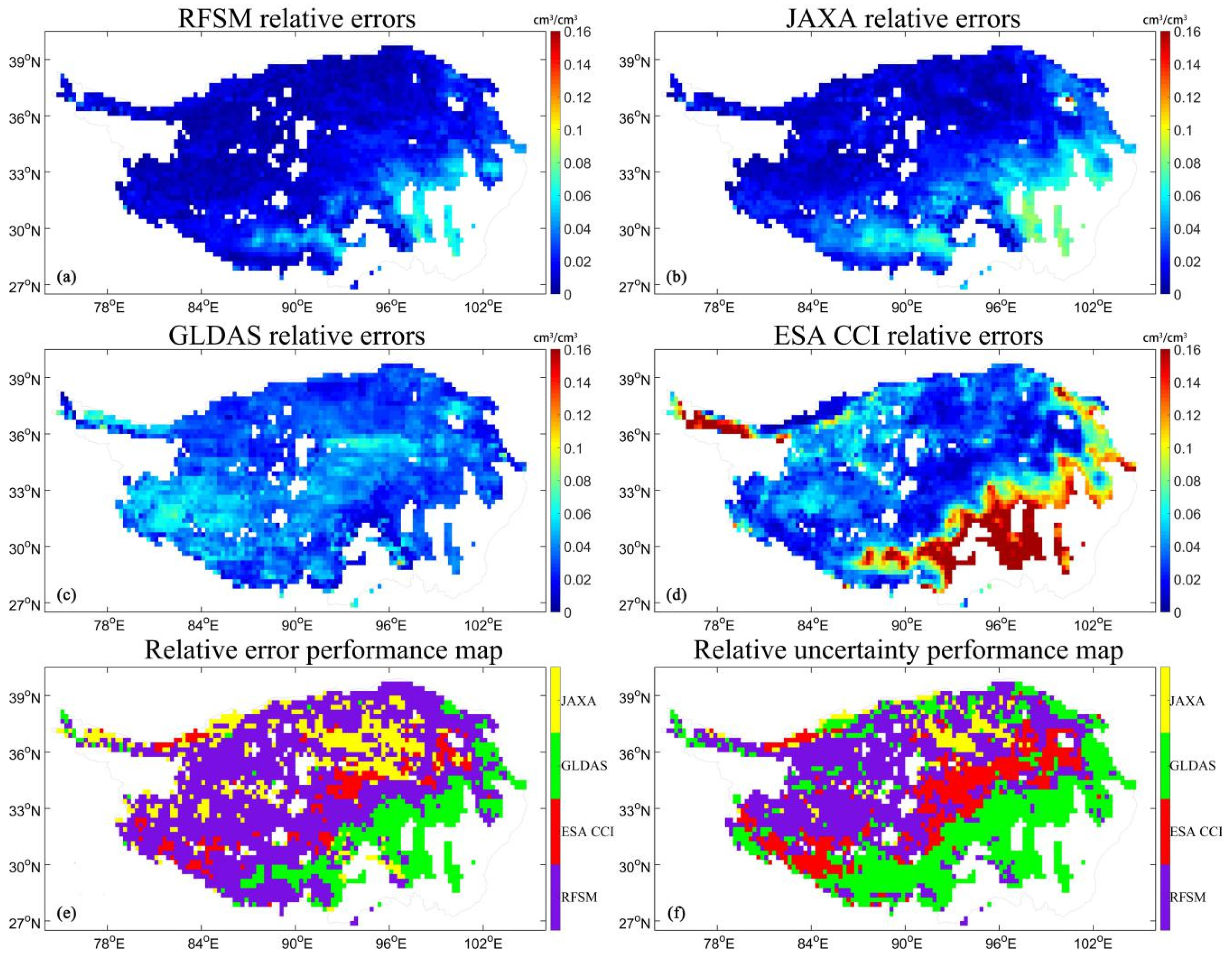
4.3.2. Spatial Distribution of RFSM

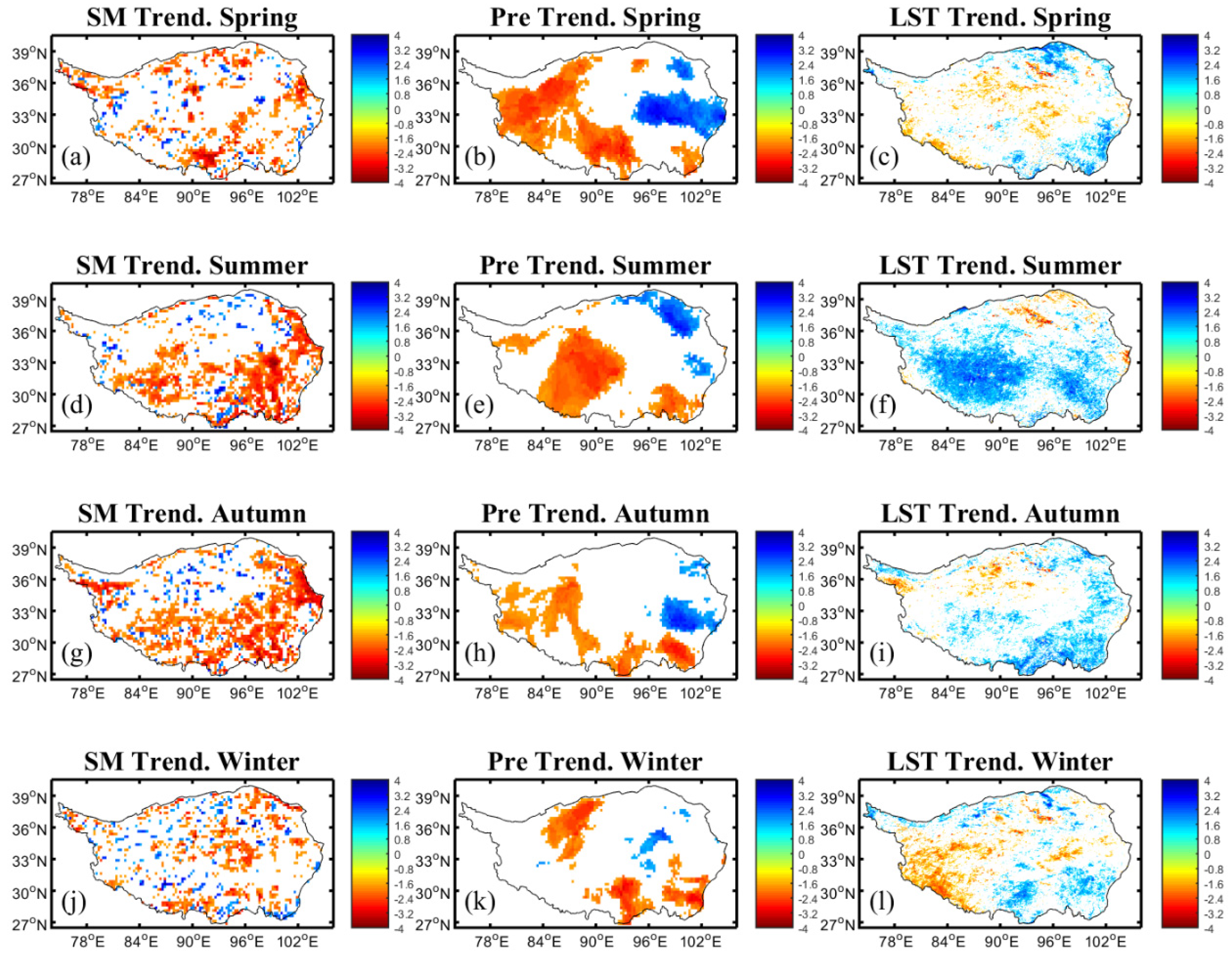
To evaluate the spatial performance of RFSM, the spatial distribution of precipitation is presented in Figure 10, and the spatial distribution diagrams over January (frozen season) and July (unfrozen season) are plotted in Figure 11 and Figure 12, respectively, using GLDAS and ESA CCI as reference data. Here, the data from 2010 and 2014 were chosen to represent the RFSM values simulated from AMSR-E and AMSR2 Tbs, respectively.

Figure 11 and Figure 12 show that the RFSM simulated from both AMSR-E and AMSR2 have the same spatial distribution patterns and similar ranges of values; together with the results analyzed in Section 4.3.1, this result indicates the successful use of AMSR-E/AMSR2 Tbs to obtain correct and consistent RFSM values from 2002 to 2015. These diagrams also show that there are almost no ESA CCI values in January, and overestimates (i.e., SM values of even higher than 0.5 m³/m³) and missing values occur in the Southeast and West of the QTP in July. However, only a few missing RFSM values are observed in January, and they fall within a rational range.

In general, the three SM products had similar spatial distributions, with high values in the Southeast and low values in the Northwest, which is consistent with the spatial distribution of precipitation shown in Figure 10. However, there were also differences between these three SM products; the ESA CCI can obviously reflect the grassland in the West corner of the QTP, but it has a tendency for overestimation. RFSM and GLDAS only have values of approximately 0.3 in this region. As shown in Figure 11, GLDAS and ESA CCI are overestimated over desert and barren lands located in the Northwestern QTP, but their RFSM values are closer to in situ data, which is the same as the results in Section 4.3.1 and Section 4.3.2. As shown in Figure 10, in July, high precipitation values occurred near Qinghai Lake in the Northeastern and Southeastern QTP, whereas low values were located in the Northwest, including Chaidamu Basin. All three products exhibit responses in the low-precipitation region, but in the high-value region, only RFSM had good performance, as GLDAS and ESA CCI exhibited smooth patterns in this region. Because GLDAS is a terrestrial modeling product using 1D water balance formulations, it can describe evapotranspiration and soil moisture processes in the vertical direction but always neglects the horizontal hydrological processes controlled by topography, geomorphology, and other conditions. These horizontal hydrological processes will introduce obvious two-dimensional features of soil moisture that have not been well described in GLDAS. Moreover, GLDAS always deals with horizontal runoff processes roughly; for example, it assumes the ground to be uniform without considering the influence of the heterogeneity of infiltration capacity and water storage capacity on runoff [69]. In addition, the ESA CCI SM product adopts a pixel-level CDF-matching approach that may modify the spatial information of the retrieval data [70]. In January, however, all three products have almost no response to precipitation because there is no liquid precipitation in winter, and snow or ice cannot be reflected in microwave soil moisture products. Only GLDAS in January 2014 can reflect the precipitation in the south central QTP, which may be caused by the fact that precipitation data are used as forcing data to retrieve soil moisture on GLDAS. However, in most regions of the QTP, we can see that RFSM and GLDAS have similar values.

4.4. Trend Analysis

By using the Mann–Kendall test, the seasonal trend of RFSM is estimated. Figure 13 shows the Z values of SM, precipitation and LST from 2002 to 2015 in spring, summer, autumn and winter respectively. Positive Z value indicates an increase trend and negative Z value indicates a decrease trend. Only the area with significant trend (α = 0.05) is shown in the figures.

Although some studies indicate that there was not a significant change in precipitation over QTP, as was shown in Figure 13, in all four seasons, precipitation has a positive trend in the northeast of QTP, while has a negative trend in the north and southwest of QTP.

As shown in Figure 13c,f,i,l, in summer and autumn, there was mainly a positive trend in LST, as for spring and winter, there was a positive trend in the north and southeast and a negative trend in southwest of QTP.

As for SM, in most region, the trend corresponds with the change of precipitation, however in the Northeast, there was an increase in precipitation and a decrease in SM in all four seasons. The trend of SM is strongly related to the change of LST. In spring, LST showed a positive trend in Northeast and Southeast, and a negative trend in Chaidamu Basin and hinterland of QTP, corresponding to the decrease of SM in Northeast and Southeast and increase of SM in Chaidamu Basin and hinterland of QTP. In summer, most regions of QTP show a positive trend of LST and negative trend of SM, and only some regions in the Northeast show a negative trend of LST and positive trend of SM. In autumn and winter, only in some North and Southwest regions as well as in the Chaidamu Basin, there was a decrease in LST and increase in SM. In other regions, there was mainly an increase in LST and decrease in SM. For SM, the positive trend was shown in some Southeast region and the West of QTP, as well as the Chaidamu Basin, and a negative trend was shown mainly in the Southeast and North of QTP, which was the same as the results of a previous study [71]. In conclusion, as for SM, there was a dryness trend in most regions of QTP and a wetness trend was only shown in some North, Southeast and Southwest regions of QTP.

5. Conclusions

In this paper, the possibility of using SMAP SM and AMSR-E/AMSR2 Tbs to simulate longer period time series and high accuracy SM over the QTP using the Random Forest method is discussed. We used Tbs data of five frequencies (double polarization of 10.7 GHz and 18.7 GHz, V polarization of 36.5 GHz) of AMSR2 from April 2015 to April 2017, as well as the longitude, latitude, DEM, IGBP, and DOY as spatial predictors to build a Random Forest model with SMAP daily SM products. Then, the deviation correction was carried out on the Tbs of AMSR-E to make them consistent with the Tbs of AMSR2. The Tbs data from June 2002 to March 2015, including AMSR-E and AMSR2, were then used to simulate RFSM.

To verify the reliability of the RF model, we simulated SM data with the Tbs of AMSR2 from April 2017 to April 2018 and compared them with SMAP. The results show that the RF model has high reliability, with high correlation (R = 0.95) and low values of RMSE (RMSE = 0.03 m³/m³) and MAPE (MAPE = 19%). However, the retrieved SM data over barren or sparsely vegetated land has a relatively poor but acceptable accuracy (R = 0.85 and MAPE = 22%), which may be due to the influence of roughness. The error distribution map shows that there is good consistency between RFSM and SMAP, with a mean RMSE value of 0.03 m³/m³, a mean bias of −0.01 m³/m³, a mean MAPE of 17% and a mean R of 0.79; the correlation is relatively poor (R = 0.5) only over bare land or around wetland. The yearly average values of SMAP SM and RFSM show that SMAP SM and RFSM have very similar spatial distributions but there is a certain degree of smoothness in RFSM. This is affected by the classification error and the fact that the final prediction of Random Forest is taken from the average values of multiple trees.

We also carried out a direct validation of these results using the traditional method. The comparison of the results between RFSM and SMAP shown in Table 3 and Table 4 indicates that RFSM maintains the value distribution of SMAP SM well but has weaker response to precipitation events than SMAP. The comparison of the results between RFSM, JAXA, LPRM, ESA CCI and GLDAS shows that RFSM exhibits reliable accuracy at all five networks, with mean values of R = 0.75, RMSE = 0.06 m³/m³, and bias = −0.03 m³/m³ over the whole year and R = 0.70, RMSE = 0.07 m³/m³, and bias = −0.05 m³/m³ over the unfrozen seasons. The scatter plot of RFSM and in situ network data also indicates that RFSM maintains special features of SMAP and has a good performance against in situ data over Naqu, Ngari and Pali, but with an underestimation around 0.35 over the uHRB and Maqu. The TCH results indicate that RFSM has the smallest relative errors in 56% of the region, with the error distribution concentrated at 0.01 m³/m³, which is the best among those of the four products (RFSM, JAXA, ESA CCI and GLDAS). This indicates that RFSM has the lowest uncertainty over the entire QTP.

The spatial distribution results show that three SM products (RFSM, GLDAS and ESA CCI) have similar spatial distributions, with high values in the Southeast and low values in the Northwest, but in some special regions, such as Qinghai Lake in the Northeast and the wetlands near the origin of the Yellow River in the eastern QTP, RFSM can reflect more details than GLDAS and ESA CCI. At the same time, RFSM exhibits very similar spatial patterns as precipitation maps in summer. The trend analysis shows that the trend of RFSM agrees well with precipitation and LST. There is a dryness trend in most region of QTP and wetness trend is only shown in some North, Southeast and Southwest regions of QTP.

In conclusion, a spatiotemporally continuous soil moisture product with high accuracy and a 14 years’ time series over the QTP was obtained from the RF model; cross-comparison shows that RFSM effectively maintains the high accuracy and spatial distribution of SMAP but prolongs the time series, and the results of validation show that RFSM performs the best out of the five SM products. However, efforts still should be made to obtain a longer-time-period RFSM product by adopting other satellite data, which will be very useful for studies of climate change over the QTP.

References

1. Entin, J.K.; Robock, A.; Vinnikov, K.Y.; Hollinger, S.E.; Liu, S.; Namkhai, A. Temporal and spatial scales of observed soil moisture variations in the extratropics. J. Geophys. Res. Atmos. 2000, 105, 11865–11877. [Google Scholar] [CrossRef]
2. Mohanty, B.P.; Cosh, M.H.; Lakshmi, V.; Montzka, C. Soil Moisture Remote Sensing: State-of-the-Science. Vadose Zone J. 2017, 16. [Google Scholar] [CrossRef]
3. Zhao, W.; Li, A. A Downscaling Method for Improving the Spatial Resolution of AMSR-E Derived Soil Moisture Product Based on MSG-SEVIRI Data. Remote Sens. Basel 2013, 5, 6790–6811. [Google Scholar] [CrossRef]
4. Zhao, L.; Yang, K.; Qin, J.; Chen, Y.; Tang, W.; Montzka, C.; Wu, H.; Lin, C.; Han, M. Spatiotemporal analysis of soil moisture observations within a Tibetan mesoscale area and its implication to regional soil moisture measurements. J. Hydrol. 2013, 482, 92–104. [Google Scholar] [CrossRef]
5. Liu, Y.Y.; Dorigo, W.A.; Parinussa, R.M.; De Jeu, R.A.M.; Wagner, W.; McCabe, M.F.; Evans, J.P.; Van Dijk, A.I.J.M. Trend-preserving blending of passive and active microwave soil moisture retrievals. Remote Sens. Environ. 2012, 123, 280–297. [Google Scholar] [CrossRef]
6. Beaudoing, H.; Rodell, M. GLDAS Noah Land Surface Model L4 3 Hourly 0.25 × 0.25 Degree V2.1; Goddard Earth Sciences Data and Information Services Center (GES DISC): Greenbelt, MD, USA, 2016. [Google Scholar]
7. Rodell, M.; Houser, P.R.; Jambor, U.; Gottschalck, J.; Mitchell, K.; Meng, C.; Arsenault, K.; Cosgrove, B.; Radakovich, J.; Bosilovich, M.; et al. The Global Land Data Assimilation System. Bull. Am. Meteorol. Soc. 2004, 85, 381–394. [Google Scholar] [CrossRef]
8. Kolassa, J.; Gentine, P.; Prigent, C.; Aires, F.; Alemohammad, S.H. Soil moisture retrieval from AMSR-E and ASCAT microwave observation synergy. Part 2: Product evaluation. Remote Sens. Environ. 2017, 195, 202–217. [Google Scholar] [CrossRef]
9. Niu, G.Y.; Yang, Z.L.; Mitchell, K.E.; Chen, F.; Ek, M.B.; Barlage, M.; Kumar, A.; Manning, K.; Niyogi, D.; Rosero, E. The community Noah land surface model with multiparameterization options (Noah-MP): 1. Model description and evaluation with local-scale measurements. J. Geophys. Res. Atmos. 2011, 116, 1248–1256. [Google Scholar] [CrossRef]
10. Kerr, Y.H.; Waldteufel, P.; Wigneron, J.P.; Delwart, S.; Cabot, F.O.; Boutin, J.; Escorihuela, M.J.; Font, J.; Reul, N.; Gruhier, C. The SMOS Mission: New Tool for Monitoring Key Elements of the Global Water Cycle. Proc. IEEE 2010, 98, 666–687. [Google Scholar] [CrossRef]
11. Entekhabi, D.; Njoku, E.G.; O’Neill, P.E.; Kellogg, K.H.; Crow, W.T.; Edelstein, W.N.; Entin, J.K.; Goodman, S.D.; Jackson, T.J.; Johnson, J.; et al. The Soil Moisture Active Passive (SMAP) Mission. Proc. IEEE 2010, 98, 704–716. [Google Scholar] [CrossRef]
12. Lorenz, C.; Montzka, C.; Jagdhuber, T.; Laux, P.; Kunstmann, H. Long-term and high-resolution global time series of brightness temperature from Copula-based fusion of SMAP Enhanced and SMOS data. Remote Sens. Basel 2018, 10, 1842. [Google Scholar] [CrossRef]
13. Zeng, J.; Chen, K.S.; Bi, H.; Chen, Q. A Preliminary Evaluation of the SMAP Radiometer Soil Moisture Product Over United States and Europe Using Ground-Based Measurements. IEEE Trans. Geosci. Remote Sens. 2016, 54, 4929–4940. [Google Scholar] [CrossRef]
14. Sun, Y.; Huang, S.; Ma, J.; Li, J.; Li, X.; Wang, H.; Chen, S.; Zang, W. Preliminary Evaluation of the SMAP Radiometer Soil Moisture Product over China Using In Situ Data. Remote Sens. Basel 2017, 9, 292. [Google Scholar] [CrossRef]
15. Ray, R.L.; Fares, A.; He, Y.; Temimi, M. Evaluation and Inter-Comparison of Satellite Soil Moisture Products Using In Situ Observations over Texas, U.S. Water 2017, 9, 372. [Google Scholar] [CrossRef]
16. Cui, H.; Jiang, L.; Du, J.; Zhao, S.; Wang, G.; Lu, Z.; Wang, J. Evaluation and analysis of AMSR-2, SMOS, and SMAP soil moisture products in the Genhe area of China. J. Geophys. Res. Atmos. 2017, 122, 8650–8666. [Google Scholar] [CrossRef]
17. Colliander, A.; Jackson, T.J.; Bindlish, R.; Chan, S.; Das, N.; Kim, S.B.; Cosh, M.H.; Dunbar, R.S.; Dang, L.; Pashaian, L. Validation of SMAP Surface Soil Moisture Products with Core Validation Sites. Remote Sens. Environ. 2017, 191, 215–231. [Google Scholar] [CrossRef]
18. Chen, Y.; Yang, K.; Qin, J.; Qian, C.; Hui, L.; Zhu, L.; Han, M.; Tang, W. Evaluation of SMAP, SMOS and AMSR2 soil moisture retrievals against observations from two networks on the Tibetan Plateau. J. Geophys. Res. Atmos. 2017, 122, 5780–5792. [Google Scholar] [CrossRef]
19. Immerzeel, W.W.; van Beek, L.P.; Bierkens, M.F. Climate change will affect the Asian water towers. Science 2010, 328, 1382–1385. [Google Scholar] [CrossRef]
20. Wu, G.; Liu, Y.; Bian, H.; Bao, Q.; Duan, A.; Jin, F.F. Thermal Controls on the Asian Summer Monsoon. Sci. Rep. UK 2012, 2, 404. [Google Scholar] [CrossRef] [PubMed]
21. Zhang, X.; Chen, N. Reconstruction of GF-1 Soil Moisture Observation Based on Satellite and In Situ Sensor Collaboration Under Full Cloud Contamination. IEEE Trans. Geosci. Remote Sens. 2016, 54, 5185–5202. [Google Scholar] [CrossRef]
22. Alyaari, A.; Bitar, A.A.; Dolman, A.; Ducharne, A.; Mialon, A.; Wigneron, J.P.; Rodriguezfernandez, N.; Richaume, P.; Jeu, R.D.; Schalie, R.V.D. Testing regression equations to derive long-term global soil moisture datasets from passive microwave observations. Remote Sens. Environ. 2016, 180, 453–464. [Google Scholar] [CrossRef]
23. Rodríguez-Fernández, N.J.; Aires, F.; Richaume, P.; Kerr, Y.H.; Prigent, C.; Kolassa, J.; Cabot, F.; Jiménez, C.; Mahmoodi, A.; Drusch, M. Soil Moisture Retrieval Using Neural Networks: Application to SMOS. IEEE Trans. Geosci. Remote Sens. 2015, 53, 5991–6007. [Google Scholar] [CrossRef]
24. Cui, Y.; Long, D.; Hong, Y.; Zeng, C.; Zhou, J.; Han, Z.; Liu, R.; Wan, W. Validation and reconstruction of FY-3B/MWRI soil moisture using an artificial neural network based on reconstructed MODIS optical products over the Tibetan Plateau. J. Hydrol. 2016, 543, 242–254. [Google Scholar] [CrossRef]
25. Yao, P.; Shi, J.; Zhao, T.; Lu, H.; Alyaari, A. Rebuilding Long Time Series Global Soil Moisture Products Using the Neural Network Adopting the Microwave Vegetation Index. Remote Sens. Basel 2017, 9, 35. [Google Scholar] [CrossRef]
26. Lu, Z.; Chai, L.; Liu, S.; Cui, H.; Zhang, Y.; Jiang, L.; Jin, R.; Xu, Z. Estimating Time Series Soil Moisture by Applying Recurrent Nonlinear Autoregressive Neural Networks to Passive Microwave Data over the Heihe River Basin, China. Remote Sens. Basel 2017, 9, 574. [Google Scholar] [CrossRef]
27. Belgiu, M.; Drăguţ, L. Random forest in remote sensing: A review of applications and future directions. ISPRS J. Photogramm. Remote Sens. 2016, 114, 24–31. [Google Scholar] [CrossRef]
28. Pal, M. Random forest classifier for remote sensing classification. Int. J. Remote Sens. 2005, 26, 217–222. [Google Scholar] [CrossRef]
29. Rodriguez-Galiano, V.F.; Ghimire, B.; Rogan, J.; Chica-Olmo, M.; Rigol-Sanchez, J.P. An assessment of the effectiveness of a random forest classifier for land-cover classification. ISPRS J. Photogramm. Remote Sens. 2012, 67, 93–104. [Google Scholar] [CrossRef]
30. Mutanga, O.; Adam, E.; Cho, M.A. High density biomass estimation for wetland vegetation using WorldView-2 imagery and random forest regression algorithm. Int. J. Appl. Earth Obs. Geoinf. 2012, 18, 399–406. [Google Scholar] [CrossRef]
31. Heung, B.; Bulmer, C.E.; Schmidt, M.G. Predictive soil parent material mapping at a regional-scale: A Random Forest approach. Geoderma 2014, 214-215, 141–154. [Google Scholar] [CrossRef]
32. Feng, Q.; Liu, J.; Gong, J. Urban Flood Mapping Based on Unmanned Aerial Vehicle Remote Sensing and Random Forest Classifier-A Case of Yuyao, China. Water 2015, 7, 1437–1455. [Google Scholar] [CrossRef]
33. Liu, X.D.; Chen, B.D. Climatic warming in the Tibetan plateau during recent decades. Int. J. Climatol. 2015, 20, 1729–1742. [Google Scholar] [CrossRef]
34. Chen, H.; Zhu, Q.; Peng, C.; Wu, N.; Wang, Y.; Fang, X.; Gao, Y.; Zhu, D.; Yang, G.; Tian, J. The impacts of climate change and human activities on biogeochemical cycles on the Qinghai-Tibetan Plateau. Glob. Chang. Biol. 2013, 19, 2940–2955. [Google Scholar] [CrossRef] [PubMed]
35. Xu, H.J.; Wang, X.P.; Zhang, X.X. Alpine grasslands response to climatic factors and anthropogenic activities on the Tibetan Plateau from 2000 to 2012. Ecol. Eng. 2016, 92, 251–259. [Google Scholar] [CrossRef]
36. Yang, K. A Multi-Scale Soil Moisture and Freeze-Thaw Monitoring Network on the Tibetan Plateau and Its Applications. Bull. Am. Meteorol. Soc. 2013, 94, 1907–1916. [Google Scholar] [CrossRef]
37. Su, Z.; Wen, J.; Dente, L.; Velde, R.V.D.; Wang, L.; Ma, Y.; Yang, K.; Hu, Z. The Tibetan Plateau observatory of plateau scale soil moisture and soil temperature (Tibet-Obs) for quantifying uncertainties in coarse resolution satellite and model products. Hydrol. Earth Syst. Sci. 2011, 15, 2303–2316. [Google Scholar] [CrossRef]
38. Ge, Y.; Wang, J.H.; Heuvelink, G.B.M.; Jin, R.; Li, X.; Wang, J.F. Sampling design optimization of a wireless sensor network for monitoring ecohydrological processes in the Babao River basin, China. Int. J. Geogr. Inf. Sci. 2015, 29, 92–110. [Google Scholar] [CrossRef]
39. Li, X.; Cheng, G.; Liu, S.; Xiao, Q.; Ma, M.; Jin, R.; Che, T.; Liu, Q.; Wang, W.; Qi, Y. Heihe Watershed Allied Telemetry Experimental Research (HiWATER): Scientific Objectives and Experimental Design. Bull. Am. Meteorol. Soc. 2013, 94, 1145–1160. [Google Scholar] [CrossRef]
40. Ma, M.; Che, T.; Li, X.; Xiao, Q.; Zhao, K.; Xin, X. A Prototype Network for Remote Sensing Validation in China. Remote Sens. Basel 2015, 7, 5187–5202. [Google Scholar] [CrossRef]
41. Jin, R.; Li, X.; Yan, B.; Li, X.; Luo, W.; Ma, M.; Guo, J.; Kang, J.; Zhu, Z.; Zhao, S. A Nested Ecohydrological Wireless Sensor Network for Capturing the Surface Heterogeneity in the Midstream Areas of the Heihe River Basin, China. IEEE Geosci. Remote Sens. Lett. 2014, 11, 2015–2019. [Google Scholar] [CrossRef]
42. Liu, S.; Li, X.; Xu, Z.; Che, T.; Xiao, Q.; Ma, M.; Liu, Q.; Jin, R.; Guo, J.; Wang, L.; et al. The Heihe Integrated Observatory Network: A basin-scale land surface processes observatory in China. Vadose Zone J. 2018, 17, 180072. [Google Scholar] [CrossRef]
43. Liu, S.; Xu, Z.; Wang, W.; Bai, J.; Jia, Z.; Zhu, M.; Wang, J. A comparison of eddy-covariance and large aperture scintillometer measurements with respect to the energy balance closure problem. Hydrol. Earth Syst. Sci. 2011, 15, 1291–1306. [Google Scholar] [CrossRef]
44. Njoku, E.G.; Chan, S.K. Vegetation and surface roughness effects on AMSR-E land observations. Remote Sens. Environ. 2006, 100, 190–199. [Google Scholar] [CrossRef]
45. Das, N.N.; Entekhabi, D.; Njoku, E.G.; Shi, J.J.C.; Johnson, J.T.; Colliander, A. Tests of the SMAP Combined Radar and Radiometer Algorithm Using Airborne Field Campaign Observations and Simulated Data. IEEE Trans. Geosci. Remote Sens. 2014, 52, 2018–2028. [Google Scholar] [CrossRef]
46. Burgin, M.S.; Colliander, A.; Njoku, E.G.; Chan, S.K.; Cabot, F.; Kerr, Y.H.; Bindlish, R.; Jackson, T.J.; Entekhabi, D.; Yueh, S.H. A Comparative Study of the SMAP Passive Soil Moisture Product with Existing Satellite-Based Soil Moisture Products. IEEE Trans. Geosci. Remote Sens 2017, 55, 2959–2971. [Google Scholar] [CrossRef]
47. O’Neill, P.E.; Chan, S.; Njoku, E.G.; Jackson, T.J.; Bindlish, R. SMAP L3 Radiometer Global Daily 36 km EASE-Grid Soil Moisture, Version 5; NASA National Snow and Ice Data Center Distributed Active Archive Center: Boulder, CO, USA, 2018. [Google Scholar]
48. Wu, J.; Gao, X.J. A gridded daily observation dataset over China region and comparison with the other datasets. Chin. J. Geophys. 2013, 56, 1102–1111. [Google Scholar]
49. Xu, Y.; Gao, X.; Shen, Y.; Xu, C.; Shi, Y.; Giorgi, A. A Daily Temperature Dataset over China and Its Application in Validating a RCM Simulation. Adv. Atmos. Sci. 2009, 26, 763–772. [Google Scholar] [CrossRef]
50. An, R.; Zhang, L.; Wang, Z.; Quaye-Ballard, J.A.; You, J.; Shen, X.; Gao, W.; Huang, L.J.; Zhao, Y.; Ke, Z. Validation of the ESA CCI soil moisture product in China. Int. J. Appl. Earth Obs. Geoinf. 2016, 48, 28–36. [Google Scholar] [CrossRef]
51. Owe, M.; Jeu, R.D.; Holmes, T. Multisensor historical climatology of satellite-derived global land surface moisture. J. Geophys. Res. Earth Surf. 2008, 113. [Google Scholar] [CrossRef]
52. Bi, H.; Ma, J.; Zheng, W.; Zeng, J. Comparison of soil moisture in GLDAS model simulations and in situ observations over the Tibetan Plateau. J. Geophys. Res. Atmos. 2016, 121, 2658–2678. [Google Scholar] [CrossRef]
53. Parinussa, R.M.; Holmes, T.R.H.; Wanders, N.; Dorigo, W.A.; De Jeu, R.A.M. A Preliminary Study toward Consistent Soil Moisture from AMSR2. J. Hydrometeorol. 2013, 16, 932–947. [Google Scholar] [CrossRef]
54. Chander, G.; Hewison, T.J.; Fox, N.; Wu, X.; Xiong, X.; Blackwell, W.J. Overview of Intercalibration of Satellite Instruments. IEEE Trans. Geosci. Remote Sens. 2013, 51, 1056–1080. [Google Scholar] [CrossRef]
55. Du, J.; Kimball, J.S.; Shi, J.; Jones, L.A.; Wu, S.; Sun, R.; Yang, H. Inter-Calibration of Satellite Passive Microwave Land Observations from AMSR-E and AMSR2 Using Overlapping FY3B-MWRI Sensor Measurements. Remote Sens. Basel 2014, 6, 8594–8616. [Google Scholar] [CrossRef]
56. Abbondanza, C.; Altamimi, Z.; Chin, T.M.; Gross, R.S.; Heflin, M.B.; Parker, J.W.; Wu, X. Three-Corner Hat for the assessment of the uncertainty of non-linear residuals of space-geodetic time series in the context of terrestrial reference frame analysis. J. Geod. 2014, 89, 313–329. [Google Scholar] [CrossRef]
57. Chin, T.M.; Gross, R.S.; Dickey, J.O. Multi-reference evaluation of uncertainty in earth orientation parameter measurements. J. Geod. 2005, 79, 24–32. [Google Scholar] [CrossRef]
58. Ferreira, V.G.; Montecino, H.D.C.; Yakubu, C.I.; Heck, B. Uncertainties of the Gravity Recovery and Climate Experiment time-variable gravity-field solutions based on three-cornered hat method. J. Appl. Remote Sens. 2016, 10, 15015. [Google Scholar] [CrossRef]
59. Lunetta, R.S.; Knight, J.F.; Ediriwickrema, J.; Lyon, J.G.; Worthy, L.D. Land-cover change detection using multi-temporal MODIS NDVI data. Remote Sens. Environ. 2009, 105, 142–154. [Google Scholar] [CrossRef]
60. Fensholt, R.; Langanke, T.; Rasmussen, K.; Reenberg, A.; Prince, S.D.; Tucker, C.; Scholes, R.J.; Quang, B.; Bondeau, A.; Eastman, R.; et al. Greenness in semi-arid areas across the globe 1981―2007―An Earth Observing Satellite based analysis of trends and drivers. Remote Sens. Environ. 2012, 121, 144–158. [Google Scholar] [CrossRef]
61. Park, S.; Im, J.; Park, S.; Rhee, J. AMSR2 soil moisture downscaling using multisensor products through machine learning approach. In Proceedings of the IEEE International Geoscience and Remote Sensing Symposium, Milan, Italy, 26–31 July 2015; pp. 1984–1987. [Google Scholar]
62. Temimi, M.; Leconte, R.; Chaouch, N.; Sukumal, P.; Khanbilvardi, R.; Brissette, F. A combination of remote sensing data and topographic attributes for the spatial and temporal monitoring of soil wetness. J. Hydrol. 2010, 388, 28–40. [Google Scholar] [CrossRef]
63. Wigneron, J.P.; Chanzy, A.; Kerr, Y.H.; Lawrence, H.; Shi, J.; Escorihuela, M.J.; Mironov, V.; Mialon, A.; Demontoux, F.; Rosnay, P.D. Evaluating an Improved Parameterization of the Soil Emission in L-MEB. IEEE Trans. Geosci. Remote Sens. 2011, 49, 1177–1189. [Google Scholar] [CrossRef]
64. Lawrence, H.; Wigneron, J.P.; Demontoux, F.; Mialon, A.; Kerr, Y. Evaluating the semi-empirical H−Q model, used to calculate the emissivity of a rough bare soil, with a numerical modeling approach. IEEE Trans. Geosci. Remote Sens. 2013, 51, 4075–4084. [Google Scholar] [CrossRef]
65. Fernandez-Moran, R.; Wigneron, J.P.; Lopez-Baeza, E.; Al-Yaari, A.; Coll-Pajaron, A.; Mialon, A.; Miernecki, M.; Parrens, M.; Salgado-Hernanz, P.M.; Schwank, M. Roughness and vegetation parameterizations at L-band for soil moisture retrievals over a vineyard field. Remote Sens. Environ. 2015, 170, 269–279. [Google Scholar] [CrossRef]
66. Liu, Y.Y.; Parinussa, R.M.; Dorigo, W.A.; Jeu, R.A.M.D.; Wagner, W.; Dijk, A.I.J.M.; Mccabe, M.F.; Evans, J.P. Developing an improved soil moisture dataset by blending passive and active microwave satellite-based retrievals. Hydrol. Earth Syst. Sci. 2011, 15, 425–436. [Google Scholar] [CrossRef]
67. Xia, Y.; Sheffield, J.; Ek, M.B.; Dong, J.; Chaney, N.; Wei, H.; Meng, J.; Wood, E.F. Evaluation of multi-model simulated soil moisture in NLDAS-2. J. Hydrol. 2014, 512, 107–125. [Google Scholar] [CrossRef]
68. Spennemann, P.C.; Rivera, J.A.; Saulo, A.C.; Penalba, O.C. A Comparison of GLDAS Soil Moisture Anomalies against Standardized Precipitation Index and Multisatellite Estimations over South America. J. Hydrometeorol. 2015, 16, 158–171. [Google Scholar] [CrossRef]
69. Bagnoud, N.; Pitman, A.J.; Mcavaney, B.J.; Holbrook, N.J. The contribution of the land surface energy balance complexity to differences in means, variances and extremes using the AMIP-II methodology. Clim. Dyn. 2005, 25, 171–188. [Google Scholar] [CrossRef]
70. Reichle, R.H.; Koster, R.D. Bias reduction in short records of satellite soil moisture. Geophys. Res. Lett. 2004, 31, 187–206. [Google Scholar] [CrossRef]
71. Lu, H.; Shi, J.C. Reconstruction and analysis of temporal and spatial variations in surface soil moisture in China using remote sensing. Chin. Sci. Bull. 2012, 57, 2824–2834. [Google Scholar] [CrossRef]
Figure 1. The locations of the sites within the Qinghai–Tibet plateau (QTP) in China.
Remotesensing 11 00683 g001
Figure 2. Flow chart of the random forest soil moisture (RFSM) product process.
Remotesensing 11 00683 g002
Figure 3. Relative variable importance of random forest based on increased mean square error (MSE). Tb36V is V polarization brightness temperature of 36.5 GHz, Tb18V is V polarization brightness temperature of 18.7 GHz, Tb18H is H polarization brightness temperature of 18.7 GHz, Tb10V is V polarization brightness temperature of 10.7 GHz, Tb10H is H polarization brightness temperature of 10.7 GHz.
Remotesensing 11 00683 g003
Figure 4. Density scatterplots for RFSM (y-axis) vs. soil moisture active passive (SMAP) soil moisture (SM) (x-axis) over the test period (May 2017 to May 2018).
Remotesensing 11 00683 g004
Figure 5. Yearly average values of (a) SMAP SM and (b) RFSM and error distribution maps of RFSM vs. SMAP SM over the test period (May 2017 to May 2018): (c) correlation coefficient ®; (d) mean absolute percentage error (MAPE); (e) root mean square error (RMSE) and (f) bias values.
Remotesensing 11 00683 g005
Figure 6. Time series of in situ network data, RFSM and Japan Aerospace Exploration Agency (JAXA), land surface parameter model (LPRM), European Space Agency’s Climate Change Initiative (ESA CCI) and Global Land Data Assimilation System (GLDAS) over a time period (2010–2015): Naqu, Maqu, Ngari, upper reach of the Heihe River Basin (uHRB) and Pali.
Remotesensing 11 00683 g006
Figure 7. Scatter plots of (a) SMAP and (b) RFSM over the uHRB, Maqu, Naqu, Ngari and Pali.
Remotesensing 11 00683 g007
Figure 8. Errors and relative uncertainties calculated by the three-cornered hat (TCH) method from 2010 to 2015: (a) RFSM relative errors; (b) JAXA relative errors; (c) GLDAS relative errors; (d) ESA CCI relative errors; (e) relative error performance map of the four products, in which the lowest relative errors are shown on the map; (f) relative uncertainty performance map of the four products, in which the lowest relative uncertainties are shown on the map.
Remotesensing 11 00683 g008
Figure 9. Distribution of the relative errors of RFSM, JAXA, GLDAS and ESA CCI calculated by the TCH method.
Remotesensing 11 00683 g009
Figure 10. Spatial distribution of precipitation in January and July of 2010 and 2014.
Remotesensing 11 00683 g010
Figure 11. Spatial distribution of RFSM, GLDAS and ESA CCI SM in 2010: (a) RFSM in Jan; (b) RFSM in Jul; (c) GLDAS in Jan; (d) GLDAS in Jul; (e) ESA CCI in Jan; (f) ESA CCI in Jul.
Remotesensing 11 00683 g011
Figure 12. Spatial distribution of RFSM, GLDAS and ESA CCI SM in 2014: (a) RFSM in Jan; (b) RFSM in Jul; (c) GLDAS in Jan; (d) GLDAS in Jul; (e) ESA CCI in Jan; (f) ESA CCI in Jul.
Remotesensing 11 00683 g012
Figure 13. Seasonal trend of SM, precipitation and land surface temperature (LST) from 2002 to 2015 with a significance level of α = 0.05: (a,d,g,j) are seasonal trends of SM in spring, summer, autumn and winter respectively; (b,e,h,k) are seasonal trends of precipitation in spring, summer, autumn and winter respectively; (c,f,i,l) are seasonal trends of LST in spring, summer, autumn and winter respectively.
Remotesensing 11 00683 g013