Wetland Classification with Multi-Angle/Temporal SAR Using Random Forests

Abstract

To better understand and mitigate threats to the long-term health and functioning of wetlands, there is need to establish comprehensive inventorying and monitoring programs. Here, remote sensing data and machine learning techniques that could support or substitute traditional field-based data collection are evaluated. For the Bay of Quinte on Lake Ontario, Canada, different combinations of multi-angle/temporal quad pol RADARSAT-2, simulated compact pol RADARSAT Constellation Mission (RCM), and high and low spatial resolution Digital Elevation and Surface Models (DEM and DSM, respectively) were used to classify six land cover classes with Random Forests: shallow water, marsh, swamp, water, forest, and agriculture/non-forested. Results demonstrate that high accuracies can be achieved with multi-temporal SAR data alone (e.g., user’s and producer’s accuracies ≥90% for a model based on a spring image and a summer image), or via fusion of SAR and DEM and DSM data for single dates/incidence angles (e.g., user’s and producer’s accuracies ≥90% for a model based on a spring image, DEM, and DSM data). For all models based on single SAR images, simulated compact pol data generally achieved lower accuracies than quad pol RADARSAT-2 data. However, it was possible to compensate for observed differences through either multi-temporal/angle data fusion or the inclusion of DEM and DSM data (i.e., as a result, there was not a statistically significant difference between multiple models). With a higher repeat-pass cycle than RADARSAT-2, RCM is expected to be a reliable source of C-band SAR data that will contribute positively to ongoing efforts to inventory wetlands and monitor change in areas containing the same land cover classes evaluated here.

1. Introduction

Wetlands provide a number of ecosystem services to both plant and animal species, including some that are at risk, threatened, or regionally rare [1]. For those that visit periodically or live permanently within them, wetlands provide habitat essential for obtaining food, procuring shelter, and breeding [2,3,4]. Humans also benefit directly from wetlands since they filter water, prevent shoreline erosion, reduce flooding and are used for recreation [5]. Nevertheless, these sensitive ecosystems continue to face pressures associated with the adverse and cumulative effects of anthropogenic disturbance, pollution, climate change, and invasive species [6,7].

Climate change specifically is expected to alter ambient temperatures, precipitation levels, and evapotranspiration rates, as well as modify and increase the variability of flow regimes [8,9]. This could affect the extent, structure, composition, and function of many wetlands, which are sensitive to changes in their hydrology [8,9,10]. For species that are adapted to certain water depths and flood durations, this is expected to impact both the quality and quantity of suitable habitat, and could create conditions that are favorable for the expansion of native generalist and/or invasive species [11]. This is especially concerning for places such as the Great Lakes Basin in North America, where invasive species such as Phragmites australis are already widespread [12].

To better understand and mitigate current and future risks to wetland ecosystems, there is a need to establish baseline conditions through comprehensive inventorying, as well as to monitor changes through time. However, effective management of wetlands is complicated by the fact that they can be both numerous and spatially extensive (e.g., in Canada, where the study area is located, wetlands make up approximately 13% of the country’s landmass or ∼1.23 million km² [13]). Further, given the dynamic nature of wetlands, there is need for frequent monitoring in order to effectively discern between the effects of short-term anomalies (e.g., abnormally wet spring), and long-term trends (e.g., changing climatic conditions). For this reason, remote sensing and/or other geospatial data, and machine learning techniques have been investigated to complement or serve as alternatives to traditional field-based data collection [14,15,16].

With increasing quantities of free data and sensors providing a range of Synthetic Aperture RADAR (SAR), optical, and Digital Elevation/Surface models (DEM and DSM, respectively), multi-source/sensor fusion has become a valuable tool for a variety of applications, including land use/land cover mapping [15,16,17,18,19,20,21]. However, there are limitations associated with relying on increasingly complex datasets, especially those that contain optical imagery that can only be acquired during cloud-free periods. This is because it can be difficult to reproduce the exact combination of data types and/or acquisition dates, especially across large geographic areas. One solution is to combine images from different seasons and/or years [16], however, results can be less informative for dynamic wetlands that can also change from year-to-year. Furthermore, to recognize trends requires several years of observations, which can be difficult to obtain.

On the other hand, SAR data are well suited for mapping and monitoring large geographic areas at high temporal frequencies, since sensors operate within the microwave region of the electromagnetic spectrum. As such, transmitted and received signals are largely unaffected by the presence of clouds and haze. This is especially advantageous for establishing baselines and evaluating change since images can be acquired under relatively comparable conditions through space and time (e.g., on anniversary dates, at similar phenological states, under similar moisture and/or inundation conditions). Nevertheless, sometimes SAR data alone are not sufficient for classifying very detailed wetland classes [19,21], although accuracies can be improved in some cases through the addition of DEM/DSM data [18].

In light of this, SAR data alone and in combination with DEM/DSM data were used to classify several wetland (shallow water, marsh, and swamp), and non-wetland (water, forest, and agricultural/non-forested uplands) land cover classes for a study area in Ontario, Canada. Using Random Forests (RF), single and multi-angle/temporal C-band RADARSAT-2 data were classified to determine the optimal incidence angle and/or acquisition timing, as well as whether accuracies can be improved via multi-angle/temporal data fusion. Then, SAR and DEM/DSM data were combined to determine whether classification accuracies can be improved. In preparation for the successor mission to RADARSAT-2—the RADARSAT Constellation Mission (RCM)—all models were also re-run following the substitution of quad (QP) for simulated compact pol (CP) data to determine whether this mode will provide relevant information for wetland inventorying and monitoring.

2. On the Use of SAR and/or DEM/DSM Data for Wetland Inventorying and Monitoring

2.1. Synthetic Aperture RADAR

SAR data can be suitable for wetland mapping and monitoring since sensors transmit and receive relatively long (i.e., compared to optical) wavelength microwaves, which can penetrate vegetation and provide information on sub canopy conditions, such as the extent of inundation. Often, backscatter returns are enhanced in the presence of inundated vegetation because little incident energy is lost via the transmission to lower layers of the surface (i.e., because of the high relative permittivity of water [22,23]). So-called double bounce scattering can also occur in cases where incident microwaves strike the horizontal saturated soil/water surface, then vertically oriented vegetation (or vice versa) before being returned to the sensor [24]. This similarly results in enhanced backscatter and/or a characteristic response that is often atypical/weaker for drier upland sites [25,26,27]. In some cases, differences in the height, structure, biomass, and other physical attributes of the vegetation can also be characterized with SAR [28], making it useful for discriminating wetlands by plant type/species [21,29].

Many remote sensing practitioners obtain much of their SAR data from the C-band RADARSAT-2 satellite, which has the capacity to collect multiple data types for a variety of applications. Of particular relevance are the different polarization settings: either linear horizontal (H) or linear vertical (V), which can number one (H or V), two (HH/HV, VV/VH, or HH/VV), or four (HH, HV, VH and VV) transmit–receive combinations. The latter so-called QP mode provides the most information about the target [30,31], and thus was evaluated in this research. Alternatively, single (SP) and dual (DP) pol data require less system power, thus can be acquired across larger swaths and/or at finer spatial resolutions. This is advantageous for some applications, although these data may not provide sufficient information to separate the land covers of interest [32].

For the upcoming RCM (scheduled to launch in 2019), C-band SAR data will continue to be provided via three identical satellites with the capacity to achieve a four-day repeat-pass cycle and near-daily global coverage. This increase in temporal coverage (relative to RADARSAT-2 with a 24-day repeat-pass cycle) could make RCM a preferred data source for wetland inventorying and monitoring. However, for RCM QP data will only be available for experiments and instead CP will be offered as a standard imaging mode. CP consists of the transmission of a single polarization and coherent reception of two orthogonal polarizations (RCM satellites will transmit in the right-hand circular (R), and will receive linear horizontal (H) and linear vertical (V)) [31]. While containing less target information than QP data, CP data also have the advantage of requiring less system power (reducing costs), while providing additional inter-channel phase information that is not available with incoherent DP data. Each RCM satellite will also operate with a higher Noise Equivalent Sigma Zero (NESZ) value than RADARSAT-2. This will impact its sensitivity to differences in backscatter, especially for low-intensity features (due to the higher proportion of noise). To assess the impact of both the difference in polarization and NESZ values on classification accuracy, simulated RCM data are also classified [33].

2.2. Digital Elevation and Surface Models

DEMs (including general elevation products and Digital Terrain or bare earth models) often provide useful information for identifying wetlands [17,20,34,35] since they are typically located in topographic depressions, where water accumulates and is retained for extended periods [36]. However, wetland inventories generated from DEMs alone can only provide baseline (static) information, as the elevation of wetlands tends to remain constant. Over the course of years or decades, however, flooding extent, plant health, and/or species composition can change dramatically (e.g., due to the propagation of an invasive species). Thus, identifying trends requires other sources of information. Alternatively, DSMs with sufficient vertical accuracy can be used to discriminate wetland types based on differences in the height of vegetation [34]. In fact, Millard and Richardson [34] found that only Light Detection and Ranging (LiDAR) data are needed to classify multiple wetland types and that model accuracy does not improve with the addition of SAR data. However, there are currently no satellite-based LiDAR sensors consistently acquiring multi-temporal DSM data. Furthermore, both DEMs and DSMs generated from high spatial resolution optical data are similarly limited in availability to cloud-free periods.

In light of these limitations, DEM and DSM data were evaluated as complementary data sources to available SAR. Throughout the study area two freely available datasets were identified and evaluated: (i) high spatial resolution DEM and DSM data derived from stereo orthophotos that are acquired on a five-year rotating schedule throughout Ontario, Canada by the Ministry of Natural Resources and Forestry (MNRF); and (ii) low spatial resolution Shuttle RADAR Topography Mission (SRTM) data, which are available near-globally, although only acquired at one time.

3. Objectives

Given the benefits of SAR data, and the potential to improve accuracies, where necessary, with DEM and DSM data, the following objectives were addressed:

(i.)

Evaluate the effect of acquisition incidence angle and timing on RF model accuracy To address this objective, multiple RF models were constructed with single SAR images acquired at different incidence angles (steep versus shallow), and during different seasons (spring versus summer), and their accuracies were compared.

(ii.)

Determine whether RF model accuracy can be improved via fusion of multi-temporal and/or multi-angle SAR data. Images used to address Objective (i) were combined as inputs to RF, and their accuracies were compared.

(iii.)

Determine whether RF model accuracy can be improved via fusion of SAR data with high or low spatial resolution DEM and DSM data. Single SAR images, and all combinations of SAR images were classified with the high spatial resolution DEM and DSM data. Select datasets were then re-processed and re-classified using the low spatial resolution DEM data, and their accuracies were compared.

(iv.)

Evaluate the effect of substituting QP RADARSAT-2 for simulated CP RCM data. All models (from Objectives (i)–(iii)) were re-run after substituting QP for simulated CP data to evaluate how accuracies were affected by the difference in information content and higher NESZ value of the latter, as well as the simulation process.

4. Study Area and Land Cover Classes

4.1. Study Area

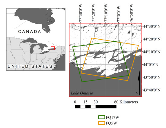
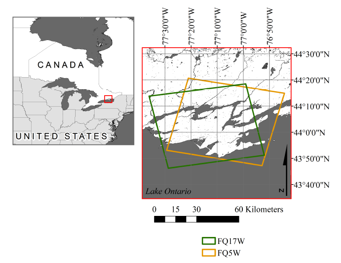
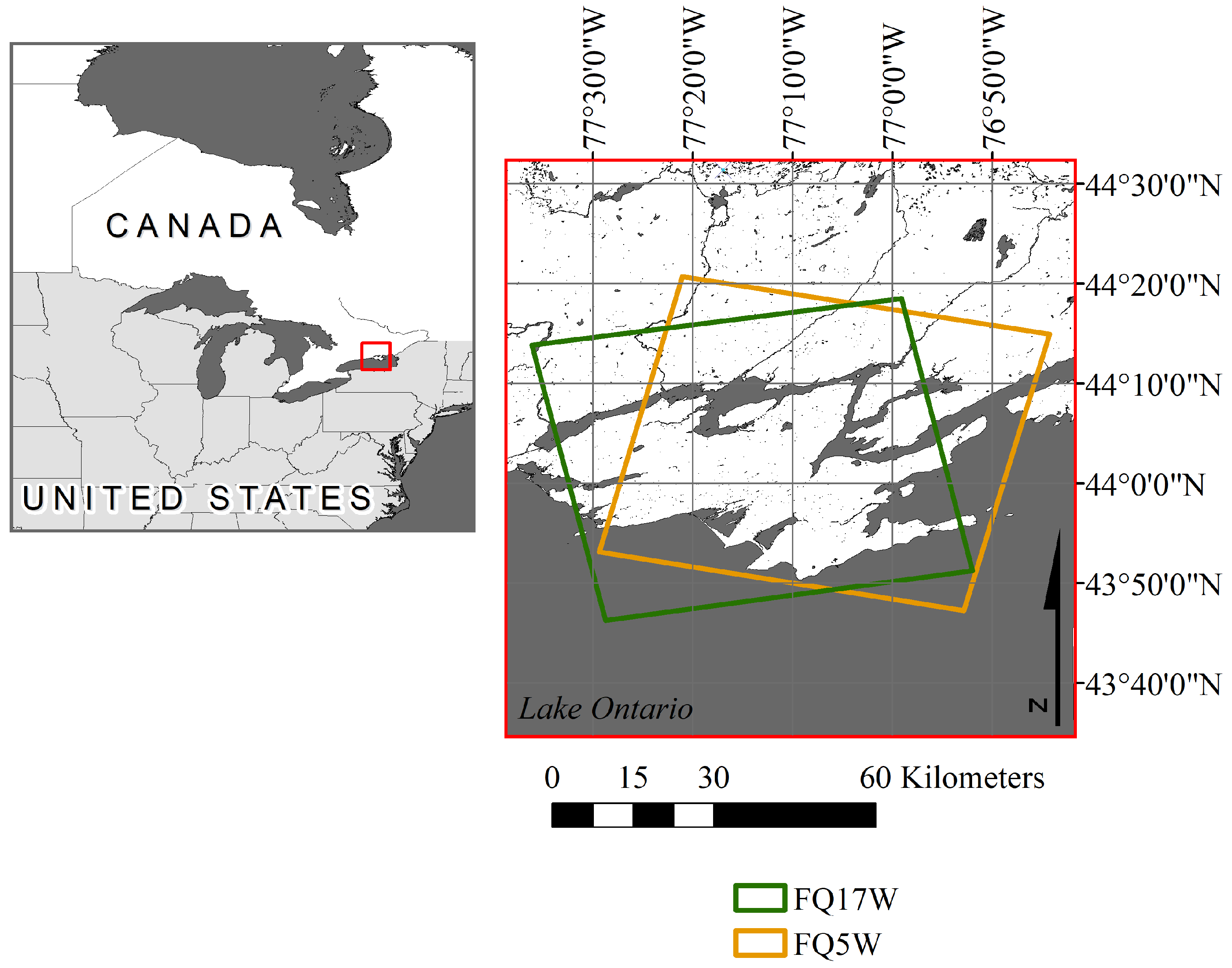
The study area is located on the Canadian side of Lake Ontario (Figure 1), and encompasses the entirety of Prince Edward County, the towns of Belleville, Shannonville, and Greater Napanee. Here, the climate is relatively mild with warm summers and cool winters. Daily average temperatures peak in July at around 21 $°$C, while rainfall is greatest for the month of September at around 90 mm [13]. The majority of the region is underlain by Paleozoic (limestone) bedrock, and glacial till. Peat, muck, and marl (organic materials) are also fairly widespread, with most located coincident with the numerous and often spatially extensive swamps and marshes present throughout the region (by comparison, shallow water wetlands are less common). Soils here are rich and fertile, thus most land is used for agricultural production, although there are many built-up areas. The local topography is mostly low-lying and flat [37].

4.2. Land Cover Classes

The Canadian Wetland Classification System [38] was used as a basis for defining the wetland types classified within the study area (

Table 1. Description of the land cover classes identified throughout the study area.

Land	Description	Training	Validation	Total
Cover		Sample	Sample
Water	All water bodies.	274	183	457
	Transitional zones between marshes and lakes that
Shallow	became densely vegetated by aquatic/emergent	59	39	98
Water	vegetation during the growing season.
Marsh	Wetlands dominated by emergent vegetation	141	94	235
	(sedges, rushes and/or reeds).
Swamp	All wetlands containing 30% or more tall woody	178	119	297
	vegetation, including shrubs/trees.
Agriculture/	All lands used for agricultural production and all	313	209	522
Non-Forested	other non-forested uplands.
Forest	Stands of coniferous and/or deciduous trees.	155	103	258
	Total	1120	747	1867

). Three general, non-wetland land covers were also classified (Table 1). Note that, for all models constructed with just spring images, it was necessary to combine the shallow water and water classes since no vegetation was present in the former until later in the growing season.

5. Data and Methods

5.1. Model Training and Validation Data

To create model training and validation data, point vectors were randomly distributed across the entire study area, and then manually labelled one of the seven land cover classes (Table 1). To do this, points were either labelled in the field during site visits in the spring, summer and fall of 2016, 2017 and 2018, or following visual interpretation of UAV (collected at various times in 2016, 2017 and 2018) or WorldView imagery (

Table 2. Acquisition dates of the data used in this research (DD/MM/YYYY).

RADARSAT-2	FQ5W: 01/05/2016 and 12/07/2016, FQ17W: 27/04/2016 and 08/07/2016
SRTM DEM	11/02/2000 to 22/02/2000
MNRF DEM/DSM	26/04/2013 to 07/05/2013 and 12/04/2015 to 23/05/2015
WorldView	14/04/2016, 27/04/2016, 23/05/2016, 04/06/2016

). In some cases, other freely available data (e.g., Landsat) were also referenced if the other imagery did not provide coverage or were acquired at an inopportune time (e.g., too early in the growing season). Points that analysts could not confidently identify were removed and new points were generated until 500 were accurately labelled. For example, if a point was located adjacent to a marsh with only spring imagery providing coverage, it was not possible to confidently identify the presence/absence of a shallow water wetland, which only becomes densely vegetated later in the growing season.

For each class, the number of points was then increased approximately proportional to the areal extent it covered [39] to maximize the number of points available for model training and validation (Table 1). To do this, analysts drew polygons throughout the study area and assigned each a class label. Points were then randomly distributed within polygons and given the same label. A small number (<5% of the total) of points were also purposefully selected (based on opportunity, and not distributed randomly) in the field using a hand-held Global Positioning System (Trimble Juno SB). All points were spaced at least 40 m apart to account for the effects of spatial autocorrelation [39], and for each class 60% were randomly selected for model training, and the remaining 40% were used for independent validation (Table 1).

5.2. Remote Sensing Data and Image Processing Details

The RADARSAT-2 satellite was programmed to acquire images at different incidence angles (i.e., 23.4–25.3$°$ and 36.4–38$°$ with the FQ5W and FQ17W beam modes, respectively), and on different dates (April, May, and July) to determine the optimal acquisition geometry and/or timing, as well as to better address the need for diverse sources of information to achieve high accuracies. Multi-angle data were acquired since steep (low) angle images often show greater sensitivity to moisture and/or inundation [40,41], while shallow (high) angle images can show greater sensitivity to the characteristics of the vegetation, including height, density, and phenology [42]. It was similarly theorized that the timing of the acquisition may be important for detecting classes such as shallow water, which only become densely vegetated later in the growing season [43], as well as for detecting inundation since the presence of leaves can result in attenuation of C-band radar at the top of the canopy [42,44]. As such, images acquired before the leafing out of the canopy and during peak of growing season conditions were evaluated (herein referred to as “spring” and “summer” imagery, respectively).

Using PCI Geomatica software (version 2017), all Single Look Complex (SLC) RADARSAT-2 images were represented as non-symmetrized scattering matrices in sigma-nought, then converted to symmetrized covariance and coherency matrices. A 5 × 5 boxcar filter was applied to reduce the effects of speckle, and several relevant variables were generated and combined into a single image (

Table 3. List of variables generated from each dataset for use in constructing RF models.

	QP		Simulated CP		DEM/DSM
1–3	HH, HV and VV Intensity	1–4	Stokes Vectors: S0, S1, S2,	1	DEM
4	Total Power (SPAN)		S3 [45]	2	Slope
5	HH/VV Intensity	5-6	Shannon Entropy:	3	Aspect
6	HV/HH Intensity		Intensity and	4	Catchment Area [46]
7	HV/VV Intensity		and Polarimetry [47]	5	Convergence Index [46]
8	Pedestal Height	7–10	RH, RV, RR, and RL	6	Valley Depth [46]
9	HH-VV Phase Difference		Intensity	7	Channel Network Base
10–13	HH, VV: Magnitude,	11	RH-RV Correlation		Level [46]
	Phase, Real, Imaginary of		Coefficient	8	Slope Length Gradient
	Correlation Coefficient	12–14	m-chi Decomposition:		Factor [46]
14–16	Freeman–Durden: Double,		Double, Volume and	9	Catchment Slope [46]
	Volume, Surface [24]		Surface Scattering [45]	10	Modified Catchment
17–20	Cloude–Pottier: Entropy,	15	Cloude AlphaS [48]		Area [46]
	Anisotropy, Alpha, Beta [49]	16	Degree of Polarization [50]	11	SAGA Wetness
21–35	Touzi Decomposition:	17	Relative Phase [30]		Index [46]
	Dominant, Secondary,	18	Conformity [50]	12	Topographic
	Tertiary: Psi, Eigenvalue,	19	Circular Polarization [30]		Wetness Index [46]
	Alpha-S, Phase, Helicity [51]		Ratio [30]	13	Relative Slope
36–39	Touzi Discriminators:				Position [46]
	Maximum, Minimum,			14	Vertical Distance to
	Difference, Polarization				Channel Network [46]
	Response [52]			15	DEM Ruggedness [46]
	Shannon Entropy: Intensity			16	DSM
40–41	and Polarimetry [47]			17	Terrain Ruggedness [46]

) [18,19,32]. Each image was orthorectified via Rational Functions, first using the satellite orbit information and the high spatial resolution (MNRF) DEM as inputs. Then, select datasets (i.e., the FQ17W spring and FQ17W summer images) were reprocessed using the low spatial resolution (SRTM) DEM (Table 2). For this research, the pixel spacing of each image was selected based on its ground range resolution (13.6 and 8.9 m for the FQ5W and FQ17W data, respectively). Following analysis of each image individually, the FQ5W and FQ17W data were combined by re-sampling the latter to the spatial resolution of the former.

Each QP image was then ingested into the RCM Simulator software developed and provided by the Canada Centre for Mapping and Earth Observation [30]. Within the simulator, CP data were synthesized by first storing the SLC RADARSAT-2 data in the Kennaugh matrix format, and then multiplying by the transmitting Stokes vector in the right-hand circular polarization. To emulate the radiometric data quality of a given RCM beam mode, a randomly generated NESZ pattern was added to the first element of this vector only (i.e., no noise was added to the phase-related parameters). The final simulated data were also stored in the Stokes vector format. For additional details and equations are provided by [30]. To reduce the effects of speckle, a 5 × 5 boxcar filter was also applied, and then several relevant variables were generated (Table 3) [19,30,32].

With relatively few training and validation samples, it was theorized that the generation of random noise (i.e., non-repeating values between simulations) could result in different classification accuracies between simulations. Thus, the simulation process was repeated six times for each RADARSAT-2 image: three times to generate three sets of high resolution mode data (NESZ pattern of $-19$ dB), and three times to generate three sets of medium resolution mode data (NESZ pattern of $-25$ dB). With four quad pol images, this resulted in 24 datasets. Each was then orthorectified using the same procedure and satellite orbital information as the original RADARSAT-2 data, and the same pixel spacing (i.e., 13.6 and 8.9 m for the FQ5W and FQ17W images, respectively). Notably, high and medium resolution mode data from RCM have a nominal pixel spacing of 5 and 16 m, respectively. However, the effects of resolution were not evaluated to avoid re-sampling of the raw RADARSAT-2 data.

The high spatial resolution (i.e., 2 m) DEM and DSM data were downloaded as rasters from the Province of Ontario’s open data catalogue—Land Information Ontario. Both were generated from 20 cm stereo orthophotos, some of which were acquired in 2013 and 2015 (combined to achieve full study area coverage) (Table 2). To the DEM, a proprietary “steam rolling” algorithm had been applied to reduced raised features, though because not all raised features were removed it is not referred to as a DTM (true bare Earth model). Only the vertical accuracies of the DSM were provided, which ranged by slope, topography, and land cover type (e.g., for open fields and deciduous trees accuracies were ±0.15 and ±6.36 m, respectively, at 95th confidence level) [53]. For both the DEM and DSM noise over water was masked using the approach described by Behnamian et al. [43]. The second version of the SRTM DEM was also downloaded as a 30 m resolution raster from the United States Geological Service’s Earth Explorer data catalogue. The vertical accuracies of this dataset are generally less than 16 m [54]. From both DEMs and the DSM several variables were generated using the System for Automated Geoscientific Analysis (Table 3) [34,46].

5.3. Applying RF and Evaluating Model Performance

All RF models were constructed in R using the randomForest package [55,56]. For each model 1000 trees were generated and default settings of randomForest were used to determine the number of variables that were tested at each node (i.e., the square root of the number of inputs), and the total number of nodes generated (i.e., unlimited). These were deemed sufficient, since during preliminary testing adjusting values did not yield higher accuracies. Since user’s and producer’s accuracies varied between different iterations of the same model (despite having the same inputs/classifier settings), the mode prediction of 10 runs (i.e., the most commonly predicted class at each pixel for 10 models) was generated and evaluated for each configuration (

Table 4. List of variables generated from each dataset for use in constructing RF models. Note that the column indicating the total number of models for CP data was calculated based on the number of simulations. For example, for models based on SAR data only, 24 different CP models were generated: for all 4 images × 3 simulations of high resolution data, and 4 images × 3 simulations of medium resolution data.

Objective	Dataset(s)	Number	Number	Number
		QP	CP	of
		Variables	Variables	Models
i/iv (SAR Data Only)	FQ5W Spring	41	19	4 QP
	FQ17W Spring	41	19	24 CP
	FQ5W Summer	41	19
	FQ17W Summer	41	19
i/iv (Multi-Angle/	FQ5W Spring and FQ5W Summer	82	38	7 QP
Temporal SAR)	FQ17W Spring and FQ17W Summer	82	38	42 CP
	FQ5W Spring and FQ17W Spring	82	38
	FQ5W Spring and FQ17W Summer	82	38
	FQ5W Summer and FQ17W Spring	82	38
	FQ5W Summer and FQ17W Summer	82	38
	All Images	164	76
iii/iv (SAR and DEM	FQ5W Spring	58	36	11 QP
/DSM Data)	FQ17W Spring	58	36	66 CP
	FQ5W Summer	58	36
	FQ17W Summer	58	36
	FQ5W Spring and FQ5W Summer	99	55
	FQ17W Spring and FQ17W Summer	99	55
	FQ5W Spring and FQ17W Spring	99	55
	FQ5W Spring and FQ17W Summer	99	55
	FQ5W Summer and FQ17W Spring	99	55
	FQ5W Summer and FQ17W Summer	99	55
	All Images	181	93

). The authors of [18,32] provided additional details on and justification for using the RF classifier, which are not repeated for brevity.

In total 154 different models (again, the mode prediction of 10 runs per dataset is treated as one model) were evaluated (Table 4) [18,32,55]. To address the objectives of this research, model accuracies were compared using: (i) independent overall accuracy (proportion of all validation points that were accurately classified); (ii) independent overall accuracy of wetlands (proportion of validation points for wetlands that were accurately classified); (iii) user’s accuracy (for a given class, the proportion of points classified as a given class that were actually that class); and (iv) producer’s accuracy (for a given class, the proportion of points accurately classified divided by the total number of validation points for that class). The McNemar’s test (95% confidence interval) [57] was also used to determine whether observed differences between models were statistically significant.

While RF runs efficiently even on relatively large datasets, it has been reported that reducing the number of variables can improve model performance [39]. To determine whether this would impact classification accuracies, the method described by Banks et al. [32] was first applied to 10 configurations selected at random (from all configurations). Highly correlated variables (r > 0.9 for spearman rho) were first grouped, and only that which had the highest Mean Decrease in Accuracy (MDA) based on 10,000 trees [43] was retained. MDA values were then recalculated and variables with the lowest importance were removed 10 at a time, until just 10 remained or accuracies decreased significantly based on the McNemar’s test (95% confidence interval) [57].

6. Results and Discussion

6.1. Effect of Reducing the Number of Variables Provided to the Model

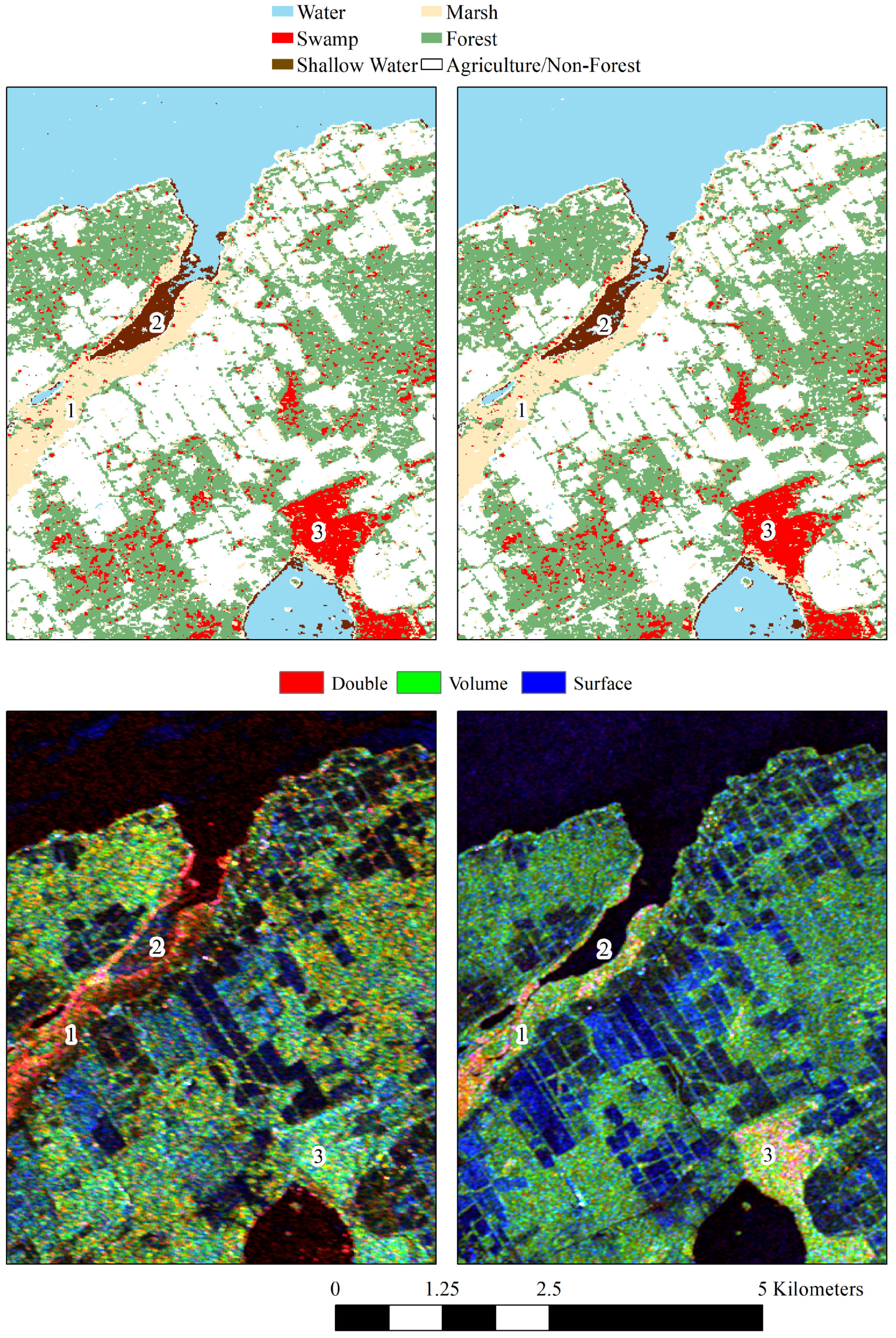
Overall, RF was observed to effectively extract relevant information from even large datasets, containing a number of variables. In all cases, decreasing the number of variables to as few as 10 did not have a statistically significant effect on model accuracy (McNemar’s test statistic; 95% confidence interval [57]). Independent overall accuracies never differed by more than 3%, and in a majority of cases user’s and producer’s accuracies differed by less than 5%, and did not always increase (note that here and throughout the manuscript the percent point or arithmetic difference is used when referring to the difference in accuracy between models). However, a 7% increase was observed for one model, although this was just for one class (shallow water). Generally, values increased for one class while decreasing for another (and vice versa), and/or user’s accuracies increased while producer’s accuracies decreased (and vice versa). Visual inspection of the final classification maps also show that models based on all or the top most important variables were comparable, especially for the majority class predicted across large wetland complexes (Figure 2). These findings are consistent with [18,32].

In light of this, effort was not made to reduce the number of variables of the other datasets (Table 4), as it was assumed that the accuracies achieved using all variables (and based on the mode of 10 runs) could provide an adequate estimate of the efficacy with which a given dataset could classify the land covers considered here. However, in the future, effort will be made to determine an optimal, reduced number of inputs because of the benefits of reduced data storage requirements and processing times.

6.2. Models Based on Single Date/Incidence Angle SAR Data

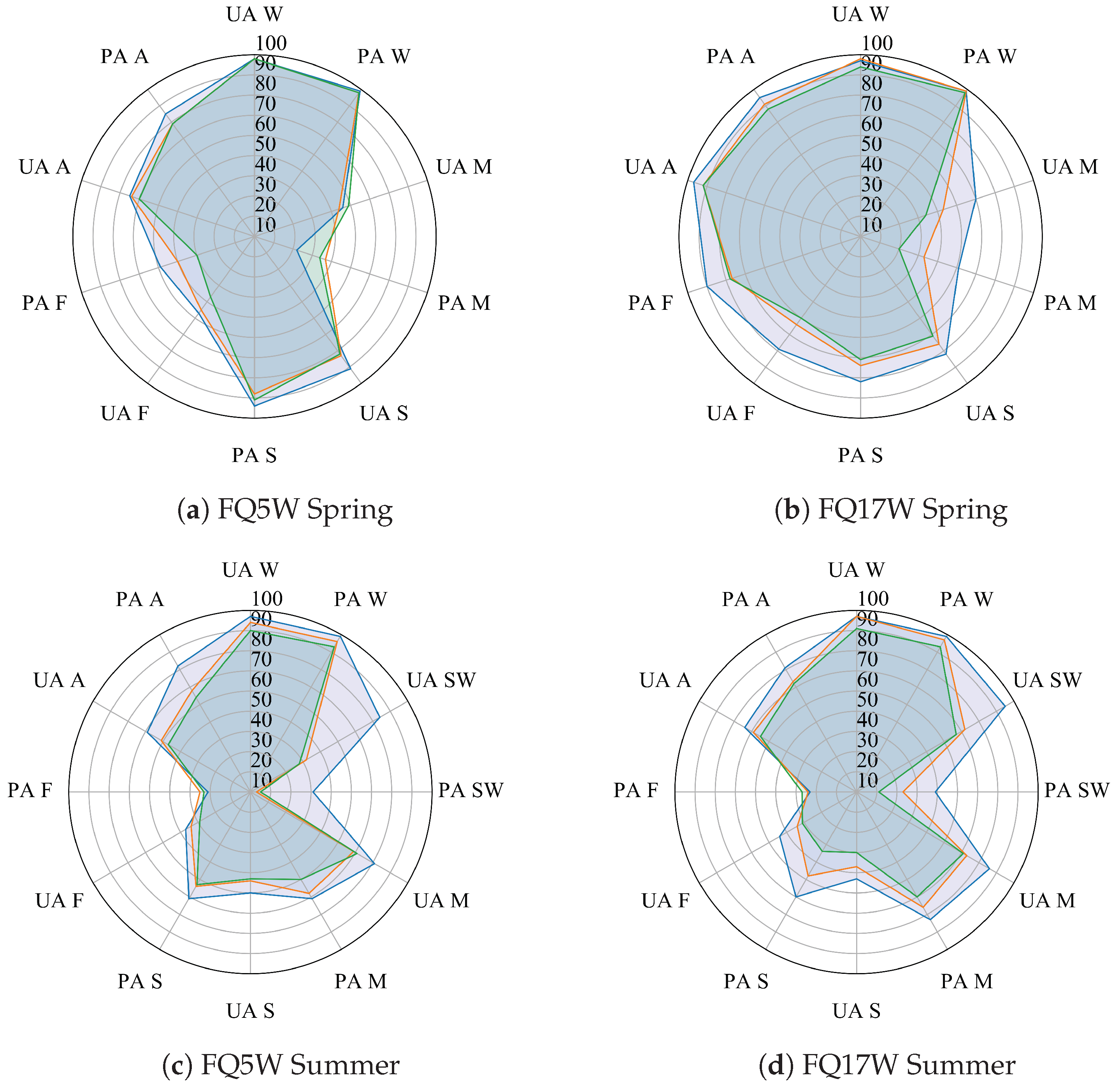
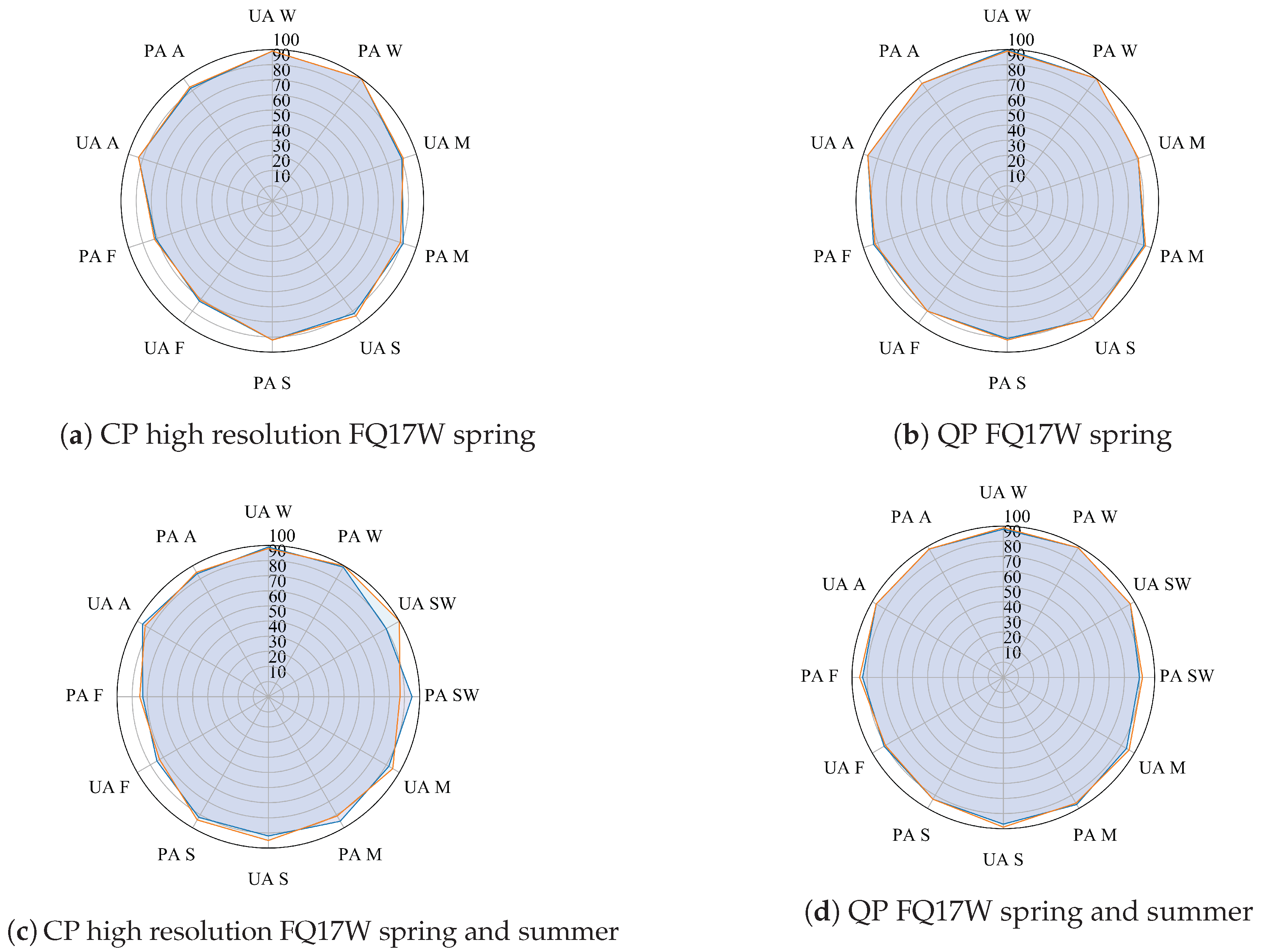
No models based on single SAR images achieved acceptable accuracies (≥∼80%) for all classes (Figure 3), though in many cases, user’s and producer’s accuracies were higher for models constructed with QP compared to CP data. This has been observed in other studies [19,32], and is attributable to the fact that the QP data contain more target information, and less noise. In most cases, accuracies were also higher for models constructed with medium compared to high resolution CP data, which is to be expected as the latter contain more noise. However, often the highest accuracy of the model based on high resolution CP data was close to or exceeded the lowest accuracy of the model based on medium resolution CP data (i.e., when considering all six simulations). Thus, it has been demonstrated that multiple simulations may be required to provide confidence in the reliability of the results.

Accuracies were often higher with high resolution CP data because of the combined effects of the quality of training/validation data (i.e., few samples in some cases), application of the NESZ pattern (random values, non-repeating between simulations), and low class separability. Specifically, for a given class, the addition of noise shifted a varying proportion of pixels either outside or within a multivariate feature space that was separable from others. This effect was also more obvious for shallow water, which had few training/validation samples, and low separability with classes like agriculture/non-forest. At least some of this variability is also attributable to the way RF randomly selects training data, and predictor variables used for node splitting though this effect was minimized by taking the mode prediction of 10 runs.

For most classes, there was less than 10% difference in the user’s and producer’s accuracies between the three sets of simulated high or three sets of medium resolution CP data. However, for forest and shallow water accuracies differed by up to 13% and 16%, respectively. However, all three simulations of high or three simulations of medium resolution data tended to misclassify the same classes (albeit at different rates), and per class accuracies were generally either relatively high or low (> or <∼80%). Therefore, only results for the first simulations are shown in Figure 3, while the following is applicable to and references results for all simulations.

Low accuracies were observed for shallow water (Figure 3), mostly because of confusion with agriculture/non-forest. This is unsurprising since in many cases both classes were observed in the field to exhibit similar surface roughness conditions. To a lesser extent, shallow water was also confused with water and marsh. This is likely because vegetation density was low in some areas (thus surface water was dominant), and because some places contained a high proportion of cattails (dominant in marshes). Models constructed with QP and CP data misclassified shallow water and agriculture/non-forest about the same number of times (i.e., 18–24 misclassifications), although the latter confused shallow water, water, and marsh more often.

For marsh high accuracies (Figure 3) were only achieved for models constructed with the QP FQ17W summer image. In contrast, accuracies were low for all models (QP and CP) based on the FQ17W spring image due to confusion between marsh and swamp. This is sensible since both classes exhibited similar backscatter characteristics in the spring (i.e., high total power attributable to double bounce and volume scattering). In the summer however, double bounce decreased more in swamps due to the leafing out of the canopy (i.e., mean values decreased 12.0 and 4.4 dB for swamp and marsh, respectively), thus making them more separable. On the other hand, accuracies for marsh were low with all FQ5W images, mostly due to confusion with agriculture/non-forest, forest, and swamp (82 and 97–102 misclassifications with QP and CP spring data, respectively; and 44 and 58–69 misclassifications with QP and CP summer data, respectively).

For swamp accuracies were high (Figure 3) for all FQ5W spring images, regardless of polarization and NESZ value. With the FQ17W spring image, lower but still acceptable accuracies were also achieved, though just with QP image. This decrease in accuracy with the FQ17W images is attributable to the fact that at shallower angles, the path length between the sensor and saturated soil/water surface is greater, increasing the number of features with which the signal interacts, and resulting in increasingly similar backscattering characteristics between flooded and non-flooded areas due to greater signal attenuation, volume and/or multiple scattering [40,41]. Notably, the lower information content and higher NESZ of the CP data appears to have compounded the effects of incidence angle, since no models based on CP FQ17W spring image achieved acceptable accuracies. Accuracies for swamp were low for all models based on summer images, since the leafing out of the canopy similarly resulted in dominant signal attenuation and volume/multiple scattering that also increased confusion with forest, especially at shallower angles (72–91 versus 47–56 misclassifications for all QP and CP models based on the FQ17W and FQ5W summer images, respectively). Thus, as was observed for marsh, the separability of swamp from other classes was similarly affected by the acquisition timing, incidence angle, polarization, and NESZ value of the SAR image.

Accuracies were high for water in all cases, indicating that this class may be less sensitive to the differences between QP and CP data. For forest, only the model constructed with the QP FQ17W spring image achieved acceptable accuracies, as this class was similarly confused with swamp in the summer. Agricultural/non-forest was only accurately classified by models based on FQ17W spring data (both QP and CP data).

6.3. Models Based on Multi-Angle/Multi-Temporal SAR Data

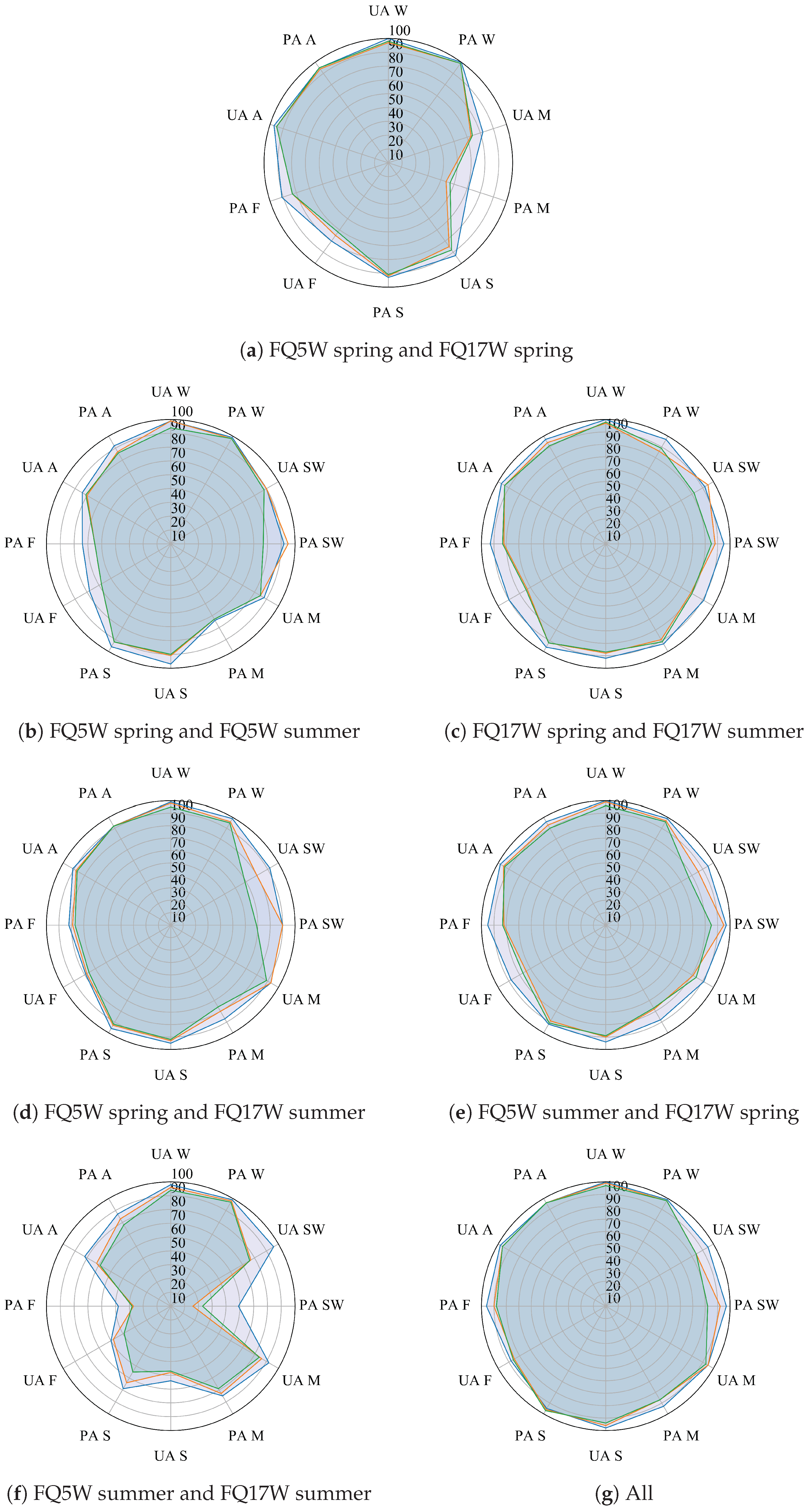
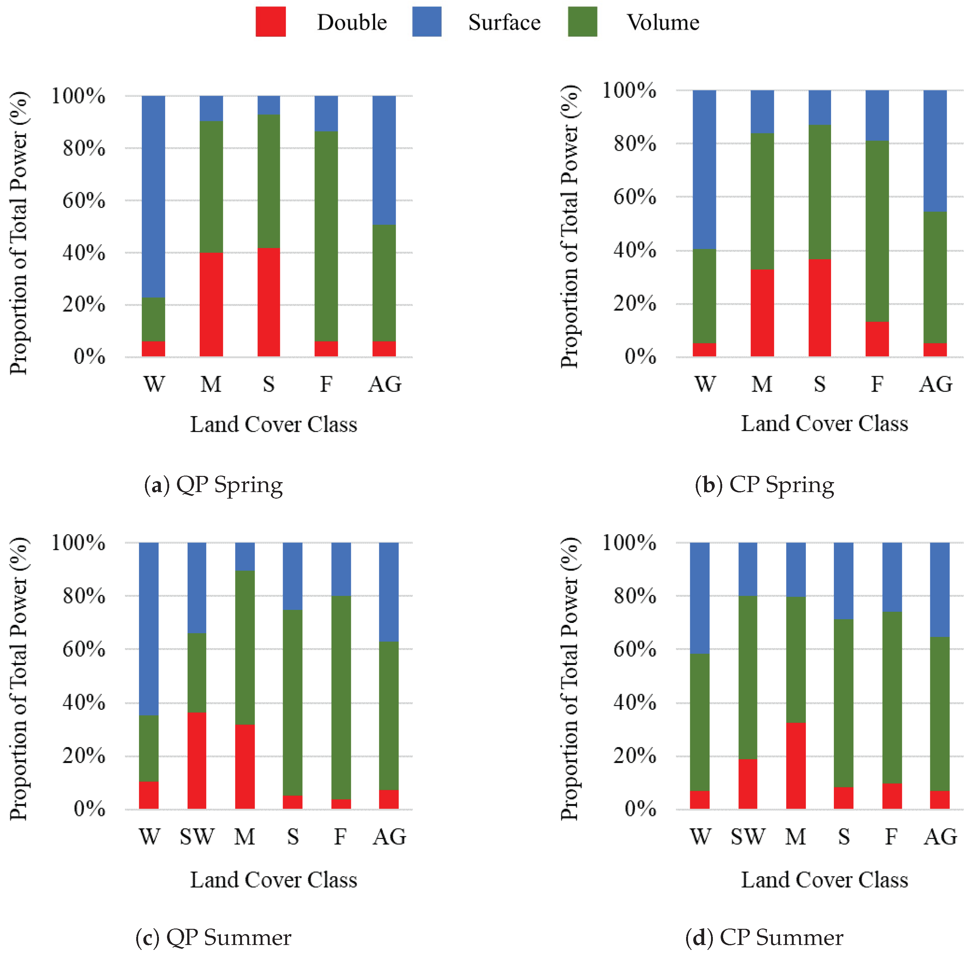
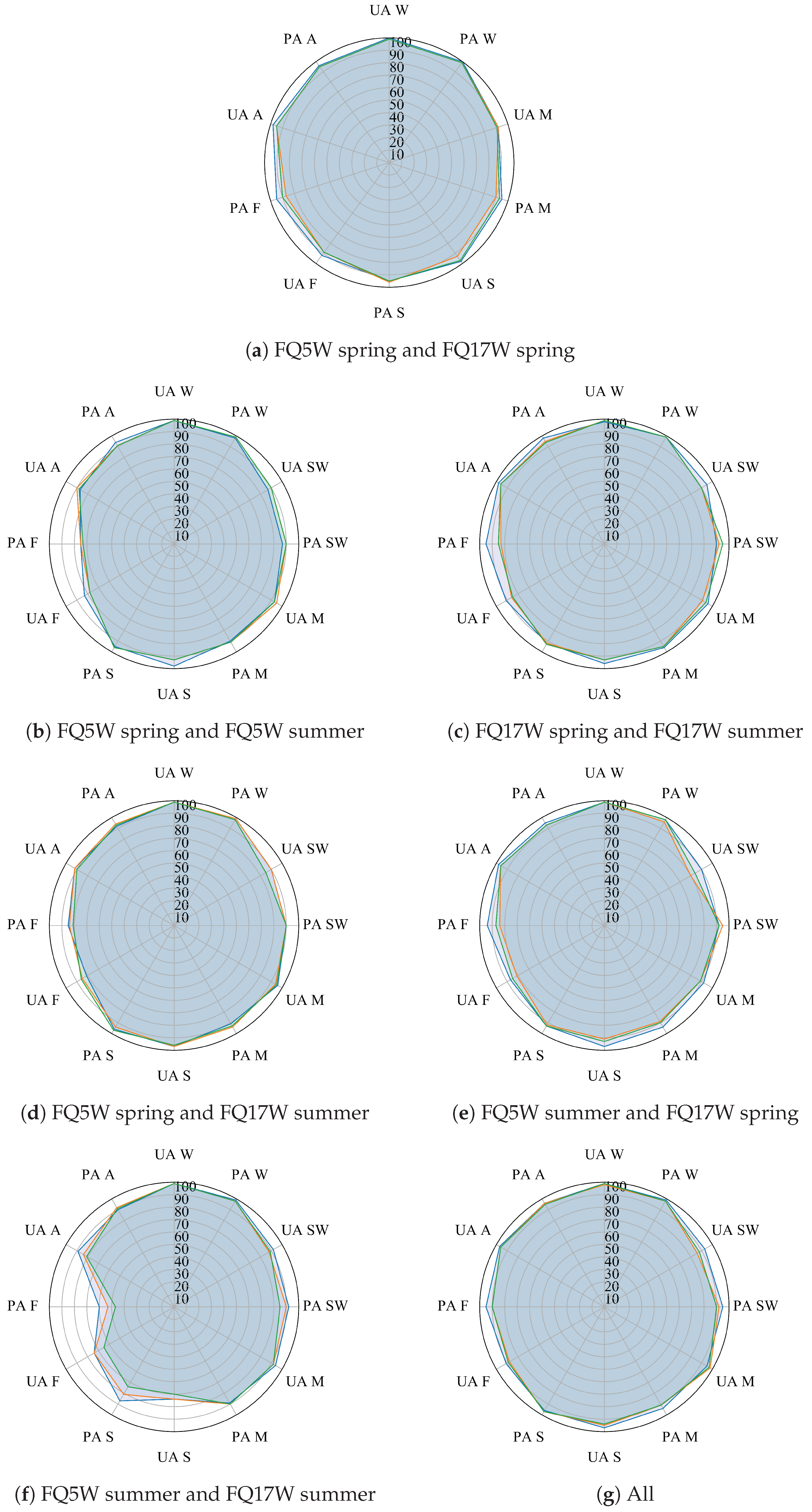
Multiple models based on two or four QP images achieved high accuracies (≥∼80%) for all classes, demonstrating the benefit of multi-temporal fusion for inventorying and monitoring wetlands (Figure 4). This increase in accuracy (relative to single SAR images) is due to multiple class pairs having similar backscatter characteristics in one, but not both seasons. For example, Figure 5 shows that for marsh and swamp the proportion of surface, double bounce, and volume scattering (Freeman–Durden or m-chi decomposition) was similar in the spring, but differed in the summer. However, values were also similar between swamp and forest in the summer, while differing in the spring. Thus, to separate all classes required information from both seasons. These results are consistent with others that have similarly demonstrated the benefit of multi-temporal SAR data for classifying wetlands [21,29]. On the other hand, multi-angle data alone appears to have been less effective for separating these classes, as accuracies were lower for models based on both spring, and especially both summer images (Figure 4). Accuracies were also lower with both FQ5W images, demonstrating preference for having at least one image acquired at a relatively shallow angle.

With CP data, only models based on all four images achieved acceptable accuracies for all classes and all simulations, demonstrating the need for more diverse sources of information to achieve high accuracies (multi-angle and multi-temporal) (

Table A1. Independent overall accuracies (IOA), independent overall accuracies for wetlands only (IOAW), and user’s (UA) and producer’s (PA) accuracies for models based on multi-angle/temporal QP, and the first (1), second (2), and third (3) simulations of high (H) and medium (M) resolution CP SAR data. Values ≤ 80% are bolded, and italicized to identify relatively high and low accuracies for a given class. Spring and summer images are abbreviated SP and SM.

Inputs	Type	IOA	OAW	W		SW		M		S		F		AG
				UA	PA	UA	PA	UA	PA	UA	PA	UA	PA	UA	PA
FQ5W SP and FQ17W SP	QP	93	84	100	100			82	71	93	93	80	91	97	95
	CP H${}^1$	89	76	98	99			74	57	88	91	72	83	95	95
	CP H${}^2$	89	77	99	99			71	59	89	92	71	83	96	94
	CP H${}^3$	89	76	98	99			73	56	87	92	75	83	95	95
	CP M${}^1$	89	75	97	99			73	54	85	92	75	83	95	94
	CP M${}^2$	89	77	99	99			71	59	89	92	71	83	96	94
	CP M${}^3$	89	76	98	99			73	56	87	92	75	83	95	95
FQ5W SP and FQ5W SM	QP	90	87	99	99	90	92	88	74	97	96	78	74	84	92
	CP H${}^1$	85	83	94	98	88	77	85	73	90	92	68	65	81	86
	CP H${}^2$	85	83	95	98	84	79	84	74	88	90	68	67	83	86
	CP H${}^3$	84	83	94	99	91	74	82	72	88	93	67	64	81	83
	CP M${}^1$	86	86	99	98	90	95	85	73	91	92	68	65	80	87
	CP M${}^2$	85	84	97	97	82	82	88	72	88	94	71	65	81	87
	CP M${}^3$	87	88	99	98	90	90	87	80	90	93	70	67	83	87
FQ17W SP and FQ17W SM	QP	95	92	99	100	97	92	95	91	93	92	90	93	97	97
	CP H${}^1$	89	84	95	98	89	82	85	80	91	87	74	83	94	91
	CP H${}^2$	88	84	96	93	92	85	89	78	87	89	75	80	89	93
	CP H${}^3$	88	85	93	93	79	77	87	79	87	92	75	81	92	91
	CP M${}^1$	90	86	99	97	86	95	88	79	89	88	73	82	94	94
	CP M${}^2$	90	85	99	99	88	92	87	80	89	87	73	81	95	94
	CP M${}^3$	91	87	99	99	90	92	86	82	89	89	75	80	95	93
FQ5W SP and FQ17W SM	QP	92	92	99	99	92	90	93	87	95	96	79	82	91	92
	CP H${}^1$	87	83	95	95	69	69	89	76	92	92	76	77	87	92
	CP H${}^2$	88	85	97	95	74	79	90	82	91	90	74	76	88	91
	CP H${}^3$	86	82	94	95	71	69	88	72	90	94	75	76	85	89
	CP M${}^1$	90	88	98	96	80	90	93	80	93	93	78	79	88	92
	CP M${}^2$	90	87	99	98	85	87	89	79	91	93	77	80	88	90
	CP M${}^3$	89	87	99	97	83	90	92	81	90	92	74	74	88	92
FQ5W SM and FQ17W SP	QP	95	92	100	99	95	97	91	88	94	92	88	95	98	96
	CP H${}^1$	89	85	96	96	77	85	84	77	89	91	77	83	94	90
	CP H${}^2$	89	81	94	98	83	77	84	72	90	90	75	83	94	92
	CP H${}^3$	89	85	94	98	82	79	82	79	89	91	79	84	95	90
	CP M${}^1$	90	86	99	97	86	95	81	78	90	89	74	82	95	93
	CP M${}^2$	89	84	96	97	82	82	79	77	87	91	76	81	96	91
	CP M${}^3$	91	87	99	98	93	97	85	77	88	92	76	83	96	93
FQ5W SM and FQ17W SM	QP	82	78	98	99	96	59	92	85	64	79	60	48	82	87
	CP H${}^1$	73	65	94	97	76	33	84	79	57	65	49	38	69	78
	CP H${}^2$	73	65	92	97	64	23	85	77	60	71	57	38	67	80
	CP H${}^3$	73	64	92	97	63	26	85	80	55	65	57	42	68	77
	CP M${}^1$	76	70	96	98	77	26	86	83	58	74	58	37	72	83
	CP M${}^2$	74	76	96	98	76	33	84	78	58	70	51	37	71	80
	CP M${}^3$	75	68	97	98	75	23	83	79	62	74	54	37	70	83
All	QP	96	94	100	99	95	97	95	93	98	95	88	96	98	96
	CP H${}^1$	94	91	97	98	84	82	93	87	94	97	86	88	96	96
	CP H${}^2$	93	90	97	99	89	82	93	88	97	93	83	88	95	95
	CP H${}^3$	94	90	98	99	87	85	94	87	95	94	84	90	96	95
	CP M${}^1$	94	92	99	98	84	92	95	87	96	96	85	90	96	96
	CP M${}^2$	94	93	99	98	88	95	93	89	96	95	83	90	97	94
	CP M${}^3$	95	94	100	99	90	95	95	89	96	97	85	90	96	95

). As was observed with single SAR images, accuracies were generally higher with medium compared to high resolution CP data, although, again, the highest accuracy among the three simulations of the high resolution data often equalled or exceeded the lowest accuracy among the three simulations of the medium resolution data. For all classes except shallow water though, differences in accuracy between the high and medium resolution CP data never exceeded 9%, and in a majority of cases the difference was less than 5%. Therefore, for these classes, there may be little benefit to acquiring medium resolution CP data at 16 m, compared to the high resolution data at 5 m, especially since both will have the same swath width (30 km).

For shallow water though more models achieved acceptable accuracies (≥∼80%), and accuracies were up to 21% higher with medium versus high resolution CP data (Table A1). However, the effects of spatial resolution similarly need to be evaluated, since this class can occupy relatively small areas, as the presence and density of vegetation can be spatially variable. Notably, because accuracies varied between simulations, so too did observed differences between models based on high or medium resolution data. For example, with the FQ5W spring and FQ17W summer models, user’s and producer’s accuracies for shallow water differed by as much as 9% and 21% (third simulation of high versus first simulation of medium), to as little as 6% and 11% (second simulation of high versus third simulation of medium). Again, this demonstrates that multiple simulations are required to provide confidence in the reliability of results.

Shallow water was also the only class for which the difference in accuracies between the three simulations of high or three simulations of medium resolution CP data exceeded 10% (maximum observed difference was 15%, although for some models differences were as low as 4%). For other classes, user’s and producer’s accuracies differed by 5% or less in a majority of cases, and, again, all simulations of high or medium resolution data generally misclassified the same classes, and accuracies tended to be relatively high or low (> or <∼80%). Therefore, Figure 4 and Figure 5 only show results for the first simulations, although all are referenced in the following section (Table A1).

With the exception of models based on both summer images, all QP and medium resolution CP datasets accurately classified shallow water (user’s and producer’s accuracies ≥∼80%). With high resolution CP data, however, only models based on all images achieved acceptable accuracies for all simulations (Table A1). It is worth mentioning that the low accuracies for models constructed with just summer data were again due mostly to confusion with agriculture/non-forest, and that, despite the combination of two angles, the number of misclassifications remained the same as models based on single SAR images (16–23 with both QP and CP data). This demonstrates the value of multi-temporal data for separating these classes.

Marsh was accurately classified (user’s and producer’s accuracies ≥∼80%) by all models based on QP data, except those constructed with just spring images, or the FQ5W spring and summer images. For the model based on spring images, accuracies were low primarily due to confusion with swamp and forest (13 and 20 misclassifications, respectively), while with the FQ5W spring and summer images confusion was mostly with forest and agriculture (10 and 16 misclassifications, respectively). Conversely, only models based on all four high or medium resolution CP images achieved acceptable accuracies for all simulations, although for multiple configurations accuracies were close to acceptable, or were acceptable for some but not all simulations.

Swamp was accurately classified by all combinations of QP and CP data (user’s and producer’s accuracies ≥84%), except when models were constructed with just summer images. For the latter, this was mostly due to confusion between swamp and forest (i.e., 57 and 50–62 misclassifications with QP and CP data, respectively), and swamp and agriculture/non-forest (i.e., 15 and 29–40 misclassifications with QP and CP data, respectively). Thus, it has been demonstrated that the availability of at least one spring image is critical for the accurate classification of swamp.

All models constructed with multi-angle/multi-temporal SAR data accurately classified water (user’s and producer’s accuracies ≥94%). On the other hand, accuracies were only high for forest with models based on QP data (user’s and producer’s accuracies ≥79%), except when constructed with the FQ5W spring and FQ5W summer imagery or the FQ5W summer and FQ17W summer images (user’s and producer’s accuracies equalled 64–78% and 48–78%, respectively). With the CP data, accuracies were only consistently high for forest when all four images were combined. Agriculture/non-forest was accurately classified by all models, except those based on CP data acquired just in the summer.

6.4. Models Based on Single SAR Images and High Spatial Resolution DEM/DSM Data

For all models constructed with single SAR images, overall accuracies increased significantly (McNemar’s test statistic; 95% confidence interval [57]) following the addition of the high spatial resolution DEM and DSM data (results for first simulation shown in Figure 6; all results provided in

Table A2. Independent overall accuracies (IOA), independent overall accuracies for wetlands only (IOAW), and user’s (UA) and producer’s (PA) accuracies for models based on single QP, and the first (1), second (2), and third (3) simulations of high (H) and medium (M) resolution CP SAR data classified in combination with the high spatial resolution DEM and DSM data. Values ≤ 80% are bolded, and italicized to identify relatively high and low accuracies for a given class. Spring and summer images are abbreviated SP and SM.

Data	Type	IOA	OAW	W		SW		M		S		F		AG
				UA	PA	UA	PA	UA	PA	UA	PA	UA	PA	UA	PA
FQ5W SP	QP	93	93	98	99			91	90	97	96	83	81	91	93
	CP H${}^1$	92	93	99	99			92	93	94	94	81	77	90	92
	CP H${}^2$	93	94	99	99			91	93	94	95	84	76	90	92
	CP H${}^3$	93	93	99	99			92	93	94	93	80	80	91	91
	CP M${}^1$	92	93	99	99			92	93	94	94	81	73	89	92
	CP M${}^2$	93	94	100	99			92	94	94	95	82	79	91	92
	CP M${}^3$	93	94	99	99			92	94	95	95	83	77	90	93
FQ17W SP	QP	96	92	100	100			91	95	96	91	90	93	97	96
	CP H${}^1$	93	92	99	100			90	91	92	92	82	81	93	92
	CP H${}^2$	94	93	100	100			91	91	89	95	88	81	93	94
	CP H${}^3$	94	94	100	100			90	94	92	94	87	83	94	93
	CP M${}^1$	94	93	99	100			92	93	92	93	86	85	96	94
	CP M${}^2$	94	92	100	100			91	91	92	93	85	83	94	93
	CP M${}^3$	94	92	99	100			91	91	92	92	84	84	95	94
FQ5W SM	QP	87	87	99	98	88	90	93	89	76	83	71	54	86	93
	CP H${}^1$	85	83	99	98	88	90	92	89	78	76	60	54	83	89
	CP H${}^2$	85	84	99	98	88	90	92	89	81	77	62	57	83	89
	CP H${}^3$	83	79	99	98	87	85	92	89	75	69	61	55	80	89
	CP M${}^1$	85	84	99	98	88	92	92	90	78	76	64	56	84	90
	CP M${}^2$	85	83	99	98	88	90	91	90	79	76	61	57	85	90
	CP M${}^3$	85	84	99	98	88	92	91	91	77	76	59	52	85	89
FQ17W SM	QP	89	90	98	99	95	92	94	94	84	86	74	65	89	93
	CP H${}^1$	87	86	99	99	92	87	92	93	81	81	69	62	87	91
	CP H${}^2$	85	84	99	99	92	90	92	93	84	83	73	64	87	92
	CP M${}^3$	88	86	99	99	92	90	93	94	82	79	70	67	88	91
	CP M${}^1$	89	88	99	99	92	90	92	93	80	83	74	67	90	92
	CP M${}^2$	88	88	99	99	92	90	92	93	84	83	73	64	87	92
	CP M${}^3$	89	87	99	99	92	92	91	91	80	82	73	66	90	92

). It is particularly notable that, for wetlands, independent overall accuracies increased by 19–39%. Despite this, accuracies were still relatively low for some classes, and only those constructed with the QP FQ5W spring, QP FQ17W spring, or CP FQ17W spring images (combined with the DEM and DSM) achieved acceptable accuracies (≥∼80%) for all classes. Accuracies were also relatively high for models constructed with the CP FQ5W spring images, DEM and DSM data, although producer’s accuracies were low in most cases for forest (ranged from 73–80%). Interestingly, the degree to which accuracies increased varied between classes and SAR images, with little to no change being observed in some cases (e.g., with QP FQ5W spring data user’s and producer’s accuracies for swamp only increased by 6% and 2% with the addition of the DEM and DSM data).

Compared to models constructed with just the single SAR images, user’s and producer’s accuracies differed less between QP and CP datasets when the DEM and DSM data was included (i.e., up to 14% and in a majority of cases <3% difference between models based on either QP, DEM and DSM data or CP, DEM and DSM data, compared to up to 55% and in a majority of cases > 10% difference between models based on just QP or CP data). There was also less of a difference between models constructed with high or medium resolution CP data (i.e., maximum of 7% and 16% when classified with, and without the DEM and DSM, respectively). This demonstrates that the DEM and DSM compensated both for the loss in information content and higher NESZ values of the CP compared to the QP data, as well as the higher NESZ value of the high compared to medium resolution CP data. With RCM then, DEM and DSM data are expected to become increasingly important as complementary data sources for wetland mapping and monitoring.

For shallow water, the addition of the DEM and DSM proved critical in improving the separability of shallow water and agriculture/non-forest, decreasing the number of misclassifications from 18–24 to 0–4 (for all QP and CP models). This is because, while both features exhibited similar backscatter characteristics, they are also located at different topographic positions (mean elevation of shallow water and agriculture non-forest is 74.4 and 93.3 m, respectively). For models based on CP data, the DEM and DSM also reduced confusion with water, and marsh (i.e., from 8–25 to 4–6 misclassifications for all models), while with QP data these classes were misclassified about the same number of times (3–8) regardless of whether DEM and DSM data was included.

Marsh was accurately classified by all models constructed with single SAR images, DEM and DSM data (user’s and producer’s accuracies ≥89%), and the range in accuracies between models was relatively low (89–95%) compared to those based on SAR data only (30–86%). This shows that these data again compensated for some of the observed differences in accuracy as a result of the timing, incidence angle, polarization and NESZ value of the SAR image. As an example, for models based on the QP FQ17W spring or QP FQ17W summer images, user’s and producer’s accuracies differed by less than 4% when the DEM and DSM was included, compared to 16% and 22% when models were constructed with just SAR data.

For swamp, user’s and producer’s accuracies were already relatively high for models constructed with images acquired in the spring, however the addition of DEM and DSM data resulted in more comparable accuracies between the FQ5W and FQ17W images compared to models based on either SAR image alone (i.e., user’s and producer’s accuracies differed by 1% and 5%, compared to 11% and 12%). This is because, for the FQ17W spring image, the DEM and DSM data reduced confusion between swamp and marsh (29 and 18–23 fewer misclassifications for models based on QP and CP data, respectively). For models based on SAR images acquired in the summer, accuracies for swamp remained low regardless of the addition of DEM and DSM data, as this did not reduce confusion with forest. This is because the DEM and DSM values for 96% of the 258 training and validation points for forest were distributed throughout the same range as values for swamp, with many for forest also being at low elevations. In light of this, it is expected that true bare Earth models and/or products with higher vertical accuracy could improve the separability between these classes.

Water was accurately classified by models constructed both with and without DEM and DSM information. Conversely, accuracies for forest remained low for models based on images acquired in the summer, because of confusion with swamp. Agriculture/non-forest was accurately classified by all models following the addition of DEM and DSM data.

6.5. Models Based on Multi-Angle/Multi-Temporal SAR Data and High Spatial Resolution DEM/DSM Data

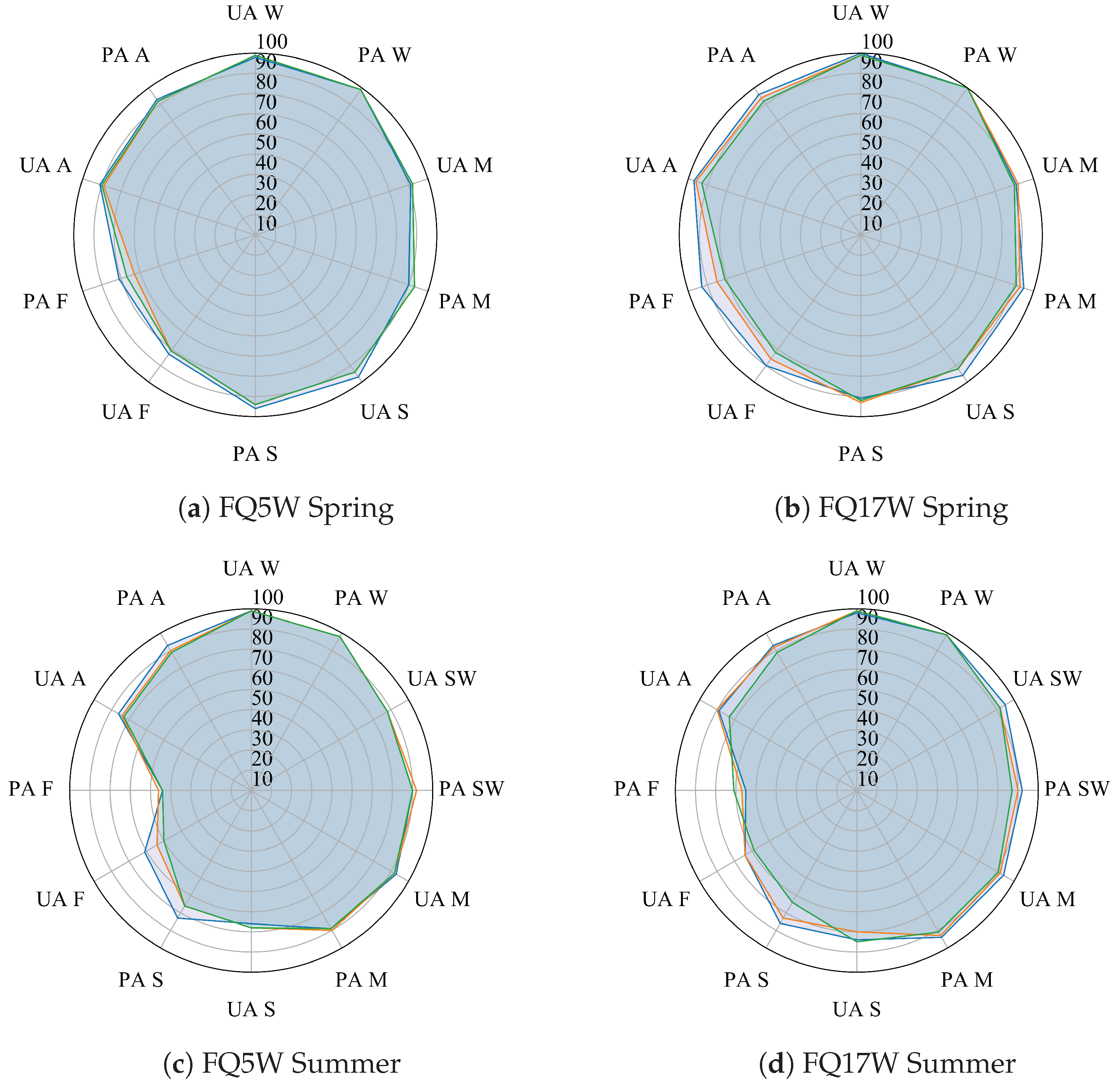
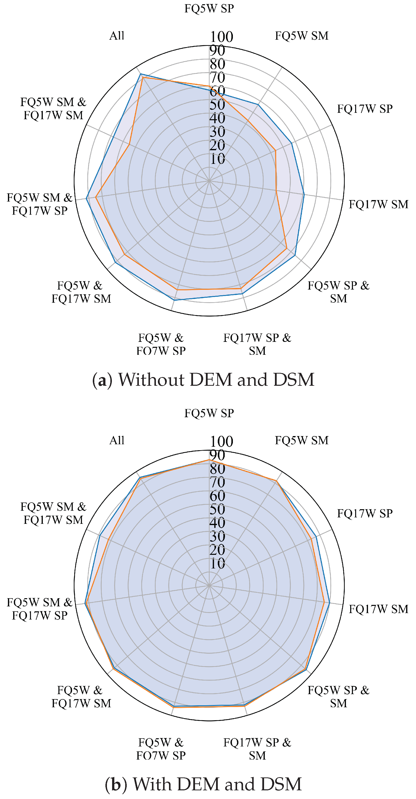
Compared to single SAR images, the addition of the DEM and DSM to models based on multi-angle/temporal SAR data had less of an effect on the overall accuracies of wetlands in some cases, which increased by 1–21% (results for first simulation shown in Figure 7; all results provided in

Table A3. Independent overall accuracies (IOA), independent overall accuracies for wetlands only (IOAW), and user’s (UA) and producer’s (PA) accuracies for models based on multi-angle/temporal QP, and the first (${}^1$), second (${}^2$), and third (${}^3$) simulations of high (H) and medium (M) resolution CP SAR data classified in combination with the high spatial resolution DEM and DSM data. Values ≤ 80% are bolded, and italicized to identify relatively high and low accuracies for a given class. Spring and summer images are abbreviated SP and SM.

Inputs	Type	IOA	OAW	W		SW		M		S		F		AG
				UA	PA	UA	PA	UA	PA	UA	PA	UA	PA	UA	PA
FQ5W SP and FQ17W SP	QP	97	95	100	100			92	95	98	95	92	95	98	96
	CP H${}^1$	95	94	99	99			91	93	97	95	89	90	95	95
	CP H${}^2$	96	94	99	100			91	94	97	94	90	91	96	95
	CP H${}^3$	95	93	99	99			91	91	97	95	89	92	96	94
	CP M${}^1$	95	93	99	99			92	90	93	96	89	87	95	95
	CP M${}^2$	95	94	100	99			91	94	95	95	88	89	96	95
	CP M${}^3$	95	94	100	99			91	94	96	95	88	91	97	94
FQ5W SP and FQ5W SM	QP	92	92	99	98	87	87	93	90	98	95	83	75	87	94
	CP H${}^1$	91	93	99	99	90	90	93	91	93	96	78	73	88	91
	CP H${}^2$	91	93	99	98	88	90	93	91	93	96	77	73	88	90
	CP H${}^3$	89	92	99	98	83	90	91	91	91	93	74	71	88	88
	CP M${}^1$	90	92	99	99	90	90	95	91	93	96	78	75	90	91
	CP M${}^2$	92	93	99	98	88	90	93	91	92	96	80	77	91	91
	CP M${}^3$	91	93	99	98	85	90	93	91	91	95	78	76	91	91
FQ17W SP and FQ17W SM	QP	96	93	98	99	95	90	96	96	96	92	91	95	98	98
	CP H${}^1$	94	94	99	99	90	95	94	95	93	93	85	85	96	94
	CP H${}^2$	94	94	99	99	90	95	91	95	91	93	88	80	95	95
	CP H${}^3$	94	92	99	99	90	92	92	95	93	91	85	85	96	95
	CP M${}^1$	94	93	99	99	90	92	91	95	93	92	86	83	96	95
	CP M${}^2$	94	95	99	99	92	92	91	96	93	95	90	83	96	95
	CP M${}^3$	94	92	99	99	90	92	92	95	93	91	85	85	96	95
FQ5W SP and FQ17W SM	QP	93	93	99	99	90	90	96	91	97	96	81	85	92	92
	CP H${}^1$	93	94	99	98	85	90	95	93	96	97	86	81	90	93
	CP H${}^2$	93	93	99	98	88	90	93	93	95	95	87	81	91	94
	CP H${}^3$	93	93	99	99	90	90	92	93	96	94	85	83	92	93
	CP M${}^1$	94	93	99	99	90	90	94	94	97	94	85	84	92	94
	CP M${}^2$	93	93	99	98	88	90	94	94	94	94	84	84	93	93
	CP M${}^3$	93	94	99	98	85	90	94	94	97	95	87	84	92	94
FQ5W SM and FQ17W SP	QP	95	93	99	98	90	92	92	94	97	93	87	94	98	95
	CP H${}^1$	93	92	99	98	84	92	89	90	93	93	85	87	96	93
	CP H${}^2$	94	93	99	98	88	92	89	94	93	93	88	85	96	94
	CP H${}^3$	94	92	99	98	88	90	89	91	94	93	88	89	96	94
	CP M${}^1$	92	92	99	96	80	95	89	89	91	92	81	84	96	93
	CP M${}^2$	94	94	99	98	88	92	90	95	94	94	87	88	97	93
	CP M${}^3$	94	94	99	98	88	92	90	94	93	95	86	86	96	93
FQ5W SM and FQ17W SM	QP	88	89	99	99	92	92	94	89	74	87	74	60	89	90
	CP H${}^1$	84	82	99	98	89	85	92	90	70	74	65	47	81	91
	CP H${}^2$	86	86	99	98	88	90	93	88	75	82	75	52	83	93
	CP H${}^3$	85	85	99	98	88	90	92	89	72	79	69	51	85	91
	CP M${}^1$	82	82	99	98	88	90	92	90	74	81	74	53	84	92
	CP M${}^2$	86	84	99	98	88	90	91	90	77	77	69	57	85	92
	CP M${}^3$	86	87	99	98	88	90	92	88	75	85	73	50	84	92
All	QP	96	95	99	99	93	95	94	94	97	96	91	97	98	96
	CP H${}^1$	95	94	98	98	88	90	97	91	94	97	89	90	96	95
	CP H${}^2$	95	94	99	98	88	90	92	94	96	96	90	90	96	95
	CP H${}^3$	95	94	99	98	88	90	93	94	95	97	90	90	97	95
	CP M${}^1$	95	94	99	98	86	92	98	91	95	97	88	90	96	96
	CP M${}^2$	95	95	99	98	88	90	93	95	96	97	90	90	97	95
	CP M${}^3$	95	96	99	99	90	90	95	96	97	97	89	90	96	94

). With QP data, accuracies only increased significantly (McNemar’s test statistic; 95% confidence interval [57]) for models based on both spring images, both summer images, and the FQ5W summer and FQ17W spring images. With CP data, however, the DEM and DSM provided additional, relevant information in a majority of cases. As a result, accuracies increased significantly for all models, except those constructed with the FQ5W spring and FQ17W summer images (one of six simulations only), both summer images (four of six simulations), or all four SAR images (all simulations).

All QP and CP models also achieved acceptable accuracies (≥80%) for all classes, with the exception of those based on the FQ5W spring and summer images, or both summer images, due to low accuracies for forest, and low accuracies for swamp, and forest, respectively. Notably, multiple configurations of just two QP or CP images, DEM and DSM data, achieved approximately the same accuracies as models based on all four QP or CP images. In contrast, when only SAR data were included as inputs, fewer models based on QP data achieved acceptable accuracies for all classes, and, with CP data, only the combination of all four images achieved acceptable accuracies for all classes and simulations. Again, this demonstrates the importance of the DEM and DSM data in achieving acceptable accuracies with CP data, but that with QP data high accuracies are possible with just multi-angle/temporal SAR data.

As was observed with single SAR images, user’s and producer’s accuracies again differed less between QP and CP models when the DEM and DSM data were included (i.e., up to 15% and in a majority of cases < 4% difference between models based multi-angle/temporal SAR, DEM and DSM data, compared to up to 36% and in a majority of cases > 7% difference between models based on just SAR data). This difference is demonstrated in Figure 8, which shows the indepednent overall accuracies of wetlands for models based on QP or the first simulation of high resolution CP imagery, classified both with and without the DEM and DSM data.

Differences in the user’s and producer’s accuracies between models based on high or medium resolution CP data were also lower (maximum of 11% compared to maximum of 21% difference when classified with and without the DEM and DSM, respectively). This again shows that these data compensated for some of the difference in information content between the QP and CP data, and between the NESZ value of the high compared to medium resolution CP data. It is worth mentioning that, between simulations of high and medium resolution data, user’s and producer’s accuracies differed by a maximum of 10%, and, in most cases, differences were less than 3%, thus only results for the first are provided in Figure 7 and Figure 8, while all are referenced in the subsequent section (Table A3).

The addition of the DEM and DSM was critical for improving accuracies for shallow water for models based on both summer images (i.e., user’s and producer’s accuracies increased from 23–96% to 88–92%). Further, while lower accuracies were often observed for shallow water with multi-angle/temporal high resolution CP data, all models accurately classified shallow water following the addition of the DEM and DSM data. Thus, this information may prove critical in cases where only high resolution data are available.

Addition of the DEM and DSM data also improved accuracies for marsh. With QP data, the DEM and DSM data were necessary for achieving acceptable accuracies for models based on images acquired just in the spring, and the FQ5W spring and summer images. With CP data, accuracies for marsh were acceptable (≥88%) for all models and all simulations with the DEM and DSM data, whereas with just SAR data, only models based on all four high or all four medium resolution images achieved acceptable accuracies for all simulations.

For swamp accuracies were high for all models based on multi-angle/temporal SAR, DEM and DSM data, except those based on just the two summer images. Notably, user’s and producer’s accuracies did increase (by 8% and 10%, respectively) following the inclusion of the DEM and DSM information, but remained relatively low (74% and 60%, respectively) due to confusion with forest.

Water, again, was accurately classified by all models, with user’s and producer’s accuracies ≥96%. Accuracies for forest, on the other hand, improved for a number of models, though remained low for those based on both FQ5W images, and both SAR images acquired in the summer. Agriculture/non-forest was accurately classified by all models, including those based on both summer images, for which accuracies were low when based just on SAR data.

6.6. Models Based on SAR Data and Low Spatial Resolution DEM Data

Given that high accuracies were observed for models based on the FQ17W spring and DEM and DSM data, and the FQ17W spring, FQ17W summer, DEM and DSM data, those QP images, and the first simulations of high resolution CP data of those images, were re-processed using the SRTM data as inputs to the orthorectification procedure. Each model was then re-run for comparison. Results from this analysis show that both models achieved acceptable accuracies, which were not significantly different (McNemar’s test statistic; 95% confidence interval [57] (Figure 9) compared to those based on the high resolution DEM and DSM data. This demonstrates that the quality of the DEM, as well as the availability of a DSM, may be less important in achieving acceptable accuracies, especially with multi-temporal SAR data.

6.7. Limitations, and Future Work

Further work is necessary to validate the results observed for the simulated RCM data (i.e., with real data), especially since the effects of resolution were not considered. This is especially true for the high resolution mode data, which may be more effective for classifying smaller wetlands, as it will be acquired at 5 m resolution. It is also notable that the NESZ values evaluated in this research are based on projected specifications, thus may differ compared to real RCM data. It is necessary to test whether these methods are transferable to other areas, for which the scattering characteristics of classes may differ. Of particular relevance is whether the high accuracies observed for swamp will also be possible in areas dominated by coniferous species, as those present in the study area contain mostly deciduous trees and/or shrubs. Future effort will also be made to address whether bogs and/or fens can be accurately classified using a similar approach. For these classes, however, the authors of [19] already demonstrated that a multi-sensor approach (including SAR, optical, and DEM data) is likely preferred. In light of this, the combination of multiple datasets (depending on the wetland types present) may be appropriate in some cases.

7. Conclusions and Future Work

Results from this analysis have provided insight regarding the effect of the timing, incidence angle, and combination of SAR and/or DEM/DSM data on RF classification accuracies for three wetland, and four non-wetland classes. High accuracies were achieved either via fusion of multi-temporal/multi-angle data, or of SAR data and DEM/DSM data, demonstrating that an efficient methodology based on one or two data sources is possible. Given that, for some combinations of data, there were no statistically significant differences in accuracy between models based on QP or simulated CP RCM imagery, it is expected to be a reliable source of C-band SAR data for inventorying and monitoring the wetland types evaluated here.

The significant conclusions of this research are as follows:

(i.)

Single date and incidence SAR data alone could not accurately classify all the land cover classes evaluated in this research, although some classes were accurately classified in some cases, with observed differences varying as a function of the acquisition timing, incidence angle, polarization, and NESZ value.

(ii.)

Multiple combinations of multi-angle/temporal QP SAR accurately classified all the land covers evaluated in this research. With CP data, more diverse sources of information were required as accuracies were only consistently high for models based on the combination of all four SAR images (multi-angle and multi-temporal data).

(iii.)

Accuracies increased significantly when DEM and DSM data were added to all models based on single SAR images, and some models based on multi-angle/temporal data. When classified with DEM and DSM data, acceptable accuracies were observed for all classes and all simulations with the FQ17W spring image, and all combinations of multi-angle/temporal data, except those based on the two FQ5W images, or the two summer images.

(iv.)

The DEM and DSM data compensated for some of the observed differences in accuracies as a result of the timing of the acquisition, its incidence angle, polarization, and NESZ value.

(v.)

High accuracies were observed regardless of whether low spatial resolution DEM or spatial resolution DEM and DSM data were used for processing the SAR data, and provided as inputs to the model.

(vi.)

High variability was observed between simulations despite using the same settings in the software, espeically for those cosntructed with single SAR images. Multiple simulations should be evaluated to provide confidence in the reliability of the results.

References

- OMNRF (Ontario Ministry of Natural Resources and Forestry). Ontario Regulation 230/08, Species at Risk in Ontario List; OMNRF: Peterborough, ON, Canada, 2018.
- Hecnar, S. Great Lakes wetlands as amphibian habitats: A review. Aquatic Ecosyst. Health Manag. 2004, 7, 289–303. [Google Scholar] [CrossRef]
- Riffell, S.K.; Keas, B.E.; Burton, T.M. Area and habitat relationships of birds in Great Lakes coastal wet meadows. Wetlands 2001, 21, 492–507. [Google Scholar] [CrossRef]
- Jude, D.J.; Pappas, J. Fish utilization of Great Lakes coastal wetlands. J. Great Lakes Res. 1992, 18, 651–672. [Google Scholar] [CrossRef]
- Kennedy, G.; Mayer, T. Natural and constructed wetlands in Canada: An overview. Water Qual. Res. J. 2002, 37, 295–325. [Google Scholar] [CrossRef]
- Dahl, T.E. Wetlands Losses in the United States, 1780’s to 1980’s; Report to the Congress; National Wetlands Inventory: St. Petersburg, FL, USA, 1990.
- Cvetkovic, M.; Chow-Fraser, P. Use of ecological indicators to assess the quality of Great Lakes coastal wetlands. Ecol. Indic. 2011, 11, 1609–1622. [Google Scholar] [CrossRef]
- Stocker, T.F.; Qin, D.; Plattner, G.; Tignor, M.; Allen, S.; Boschung, J.; Nauels, A.; Xia, Y.; Bex, V.; Midgley, P. Climate Change 2013: The Physical Science Basis. Intergovernmental Panel on Climate Change, Working Group I Contribution to the IPCC Fifth Assessment Report (AR5); Cambridge University Press: Cambridge, UK; New York, NY, USA, 2013. [Google Scholar]
- Impacts, A. Vulnerability. Part A: Global and Sectoral Aspects. Contribution of Working Group II to the Fifth Assessment Report of the Intergovernmental Panel on Climate Change; Cambridge University Press: Cambridge, UK; New York, NY, USA, 2014. [Google Scholar]
- Ontario’s Biodiversity Council. Report on the State of Ontario’s Biodiversity 2015; Ontario’s Biodiversity Council: Peterborough, ON, Canada, 2015. [Google Scholar]
- Ficke, A.D.; Myrick, C.A.; Hansen, L.J. Potential impacts of global climate change on freshwater fisheries. Rev. Fish Biol. Fish. 2007, 17, 581–613. [Google Scholar] [CrossRef]
- Bolton, R.M.; Brooks, R.J. Impact of the seasonal invasion of Phragmites australis (common reed) on turtle reproductive success. Chelonian Conserv. Biol. 2010, 9, 238–243. [Google Scholar] [CrossRef]
- Environment and Climate Change Canada. Canadian Climate Normals 1981:2010; Environment and Climate Change Canada: Gatineau, QC, Canada, 2018.
- Li, J.; Chen, W. A rule-based method for mapping Canada’s wetlands using optical, radar and DEM data. Int. J. Remote Sens. 2005, 26, 5051–5069. [Google Scholar] [CrossRef]
- Corcoran, J.M.; Knight, J.F.; Gallant, A.L. Influence of multi-source and multi-temporal remotely sensed and ancillary data on the accuracy of random forest classification of wetlands in Northern Minnesota. Remote Sens. 2013, 5, 3212–3238. [Google Scholar] [CrossRef]
- Bourgeau-Chavez, L.; Endres, S.; Battaglia, M.; Miller, M.E.; Banda, E.; Laubach, Z.; Higman, P.; Chow-Fraser, P.; Marcaccio, J. Development of a bi-national Great Lakes coastal wetland and land use map using three-season PALSAR and Landsat imagery. Remote Sens. 2015, 7, 8655–8682. [Google Scholar] [CrossRef]
- Corcoran, J.; Knight, J.; Brisco, B.; Kaya, S.; Cull, A.; Murnaghan, K. The integration of optical, topographic, and radar data for wetland mapping in northern Minnesota. Can. J. Remote Sens. 2012, 37, 564–582. [Google Scholar] [CrossRef]
- Banks, S.; Millard, K.; Pasher, J.; Richardson, M.; Wang, H.; Duffe, J. Assessing the potential to operationalize shoreline sensitivity mapping: Classifying multiple Wide Fine Quadrature Polarized RADARSAT-2 and Landsat 5 scenes with a single Random Forest model. Remote Sens. 2015, 7, 13528–13563. [Google Scholar] [CrossRef]
- White, L.; Millard, K.; Banks, S.; Richardson, M.; Pasher, J.; Duffe, J. Moving to the RADARSAT constellation mission: Comparing synthesized compact polarimetry and dual polarimetry data with fully polarimetric RADARSAT-2 data for image classification of peatlands. Remote Sens. 2017, 9, 573. [Google Scholar] [CrossRef]
- Amani, M.; Salehi, B.; Mahdavi, S.; Granger, J.E.; Brisco, B.; Hanson, A. Wetland classification using multi-source and multi-temporal optical remote sensing data in Newfoundland and Labrador, Canada. Can. J. Remote Sens. 2017, 43, 360–373. [Google Scholar] [CrossRef]
- Mahdavi, S.; Salehi, B.; Amani, M.; Granger, J.E.; Brisco, B.; Huang, W.; Hanson, A. Object-based classification of wetlands in Newfoundland and Labrador using multi-temporal PolSAR data. Can. J. Remote Sens. 2017, 43, 432–450. [Google Scholar] [CrossRef]
- Henderson, F.; Lewis, A.J. Principles and Applications of Imaging Radar. Manual of Remote Sensing: Volume 2; John Wiley and Sons, Inc.: Somerset, NJ, USA, 1998. [Google Scholar]
- Sun, G.; Simonett, D.S.; Strahler, A.H. A radar backscatter model for discontinuous coniferous forests. IEEE Trans. Geosci. Remote Sens. 1991, 29, 639–650. [Google Scholar] [CrossRef]
- Freeman, A.; Durden, S.L. A three-component scattering model for polarimetric SAR data. IEEE Trans. Geosci. Remote Sens. 1998, 36, 963–973. [Google Scholar] [CrossRef]
- Hess, L.L.; Melack, J.M.; Simonett, D.S. Radar detection of flooding beneath the forest canopy: A review. Int. J. Remote Sens. 1990, 11, 1313–1325. [Google Scholar] [CrossRef]
- Brisco, B.; Touzi, R.; van der Sanden, J.J.; Charbonneau, F.; Pultz, T.; D’Iorio, M. Water resource applications with RADARSAT-2—A preview. Int. J. Digit. Earth 2008, 1, 130–147. [Google Scholar] [CrossRef]
- Brisco, B.; Kapfer, M.; Hirose, T.; Tedford, B.; Liu, J. Evaluation of C-band polarization diversity and polarimetry for wetland mapping. Can. J. Remote Sens. 2011, 37, 82–92. [Google Scholar] [CrossRef]
- Gallant, A.L.; Kaya, S.G.; White, L.; Brisco, B.; Roth, M.F.; Sadinski, W.; Rover, J. Detecting emergence, growth, and senescence of wetland vegetation with polarimetric synthetic aperture radar (SAR) data. Water 2014, 6, 694–722. [Google Scholar] [CrossRef]
- Gosselin, G.; Touzi, R.; Cavayas, F. Polarimetric Radarsat-2 wetland classification using the Touzi decomposition: Case of the Lac Saint-Pierre Ramsar wetland. Can. J. Remote Sens. 2014, 39, 491–506. [Google Scholar] [CrossRef]
- Charbonneau, F.; Brisco, B.; Raney, R.; McNairn, H.; Liu, C.; Vachon, P.; Shang, J.; DeAbreu, R.; Champagne, C.; Merzouki, A.; et al. Compact polarimetry overview and applications assessment. Can. J. Remote Sens. 2010, 36, S298–S315. [Google Scholar] [CrossRef]
- Raney, R.K. Hybrid-Polarity SAR Architecture. IEEE Trans. Geosci. Remote Sens. 2007, 45, 3397–3404. [Google Scholar] [CrossRef]
- Banks, S.; Millard, K.; Behnamian, A.; White, L.; Ullmann, T.; Charbonneau, F.; Chen, Z.; Wang, H.; Pasher, J.; Duffe, J. Contributions of Actual and Simulated Satellite SAR Data for Substrate Type Differentiation and Shoreline Mapping in the Canadian Arctic. Remote Sens. 2017, 9, 1206. [Google Scholar] [CrossRef]
- Thompson, A. Overview of the RADARSAT constellation mission. Can. J. Remote Sens. 2015, 41, 401–407. [Google Scholar] [CrossRef]
- Millard, K.; Richardson, M. Wetland mapping with LiDAR derivatives, SAR polarimetric decompositions, and LiDAR–SAR fusion using a random forest classifier. Can. J. Remote Sens. 2013, 39, 290–307. [Google Scholar] [CrossRef]
- Hird, J.N.; DeLancey, E.R.; McDermid, G.J.; Kariyeva, J. Google Earth Engine, open-access satellite data, and machine learning in support of large-area probabilistic wetland mapping. Remote Sens. 2017, 9, 1315. [Google Scholar] [CrossRef]
- Tiner, R.W. Wetland indicators: A guide to wetland identification. In Delineation, Classification, and Mapping; CRC Press: Boca Raton, FL, USA, 1999. [Google Scholar]
- Ontario Ministry of Energy, Northern Development and Mines. Surficial Geology of Southern Ontario; Ontario Ministry of Energy, Northern Development and Mines: Greater Sudbury, ON, Canada, 2012.
- The Canadian Wetland Classification System; Environment and Climate Change Canada: Gatineau, QC, Canada, 1997.
- Millard, K.; Richardson, M. On the importance of training data sample selection in Random Forest image classification: A case study in peatland ecosystem mapping. Remote Sens. 2015, 7, 8489–8515. [Google Scholar] [CrossRef]
- Lunetta, R.S.; Elvidge, C.D. Remote Sensing Change Detection; Taylor & Francis: Boca Raton, FL, USA, 1999; Volume 310. [Google Scholar]
- Lang, M.W.; Townsend, P.A.; Kasischke, E.S. Influence of incidence angle on detecting flooded forests using C-HH synthetic aperture radar data. Remote Sens. Environ. 2008, 112, 3898–3907. [Google Scholar] [CrossRef]
- Henderson, F.M.; Lewis, A.J. Radar detection of wetland ecosystems: A review. Int. J. Remote Sens. 2008, 29, 5809–5835. [Google Scholar] [CrossRef]
- Behnamian, A.; Banks, S.; White, L.; Brisco, B.; Milard, K.; Pasher, J.; Chen, Z.; Duffe, J.; Bourgeau-Chavez, L.; Battaglia, M. Semi-Automated Surface Water Detection with Synthetic Aperture Radar Data: A Wetland Case Study. Remote Sens. 2017, 9, 1209. [Google Scholar] [CrossRef]
- Townsend, P. Relationships between forest structure and the detection of flood inundation in forested wetlands using C-band SAR. Int. J. Remote Sens. 2002, 23, 443–460. [Google Scholar] [CrossRef]
- Raney, R.K.; Cahill, J.T.; Patterson, G.; Bussey, D.B.J. The m-chi decomposition of hybrid dual-polarimetric radar data with application to lunar craters. J. Geophys. Res. Planets 2012, 117. [Google Scholar] [CrossRef]
- Conrad, O.; Bechtel, B.; Bock, M.; Dietrich, H.; Fischer, E.; Gerlitz, L.; Wehberg, J.; Wichmann, V.; Böhner, J. System for Automated Geoscientific Analyses (SAGA) v. 2.1.4. Geosci. Model Dev. 2015, 8, 1991–2007. [Google Scholar] [CrossRef]
- Lee, J.S.; Pottier, E. Polarimetric Radar Imaging From Basics to Applications; CRC Press: Boca Raton, FL, USA, 2009. [Google Scholar]
- Cloude, S.R.; Goodenough, D.G.; Chen, H. Compact Decomposition Theory. IEEE Geosci. Remote Sens. Lett. 2012, 9, 28–32. [Google Scholar] [CrossRef]
- Cloude, S.R.; Pottier, E. An entropy based classification scheme for land applications of polarimetric SAR. IEEE Trans. Geosci. Remote Sens. 1997, 35, 68–78. [Google Scholar] [CrossRef]
- Truong-Loi, M.L.; Freeman, A.; Dubois-Fernandez, P.C.; Pottier, E. Estimation of soil moisture and Faraday rotation from bare surfaces using compact polarimetry. IEEE Trans. Geosci. Remote Sens. 2009, 47, 3608–3615. [Google Scholar] [CrossRef]
- Touzi, R. Target scattering decomposition in terms of roll-invariant target parameters. IEEE Trans. Geosci. Remote Sens. 2007, 45, 73–84. [Google Scholar] [CrossRef]
- Touzi, R.; Goze, S.; Le Toan, T.; Lopes, A.; Mougin, E. Polarimetric discriminators for SAR images. IEEE Trans. Geosci. Remote Sens. 1992, 30, 973–980. [Google Scholar] [CrossRef]
- Provincial Mapping Unit; Mapping and Information Resources Branch; Corporate Management and Information Division; Ministry of Natural Resources and Forestry. Vertical Accuracy Assessment; Queen’s Printer for Ontario: Los Angeles, CA, USA, 2017.
- Elkhrachy, I. Vertical accuracy assessment for SRTM and ASTER Digital Elevation Models: A case study of Najran city, Saudi Arabia. Ain Shams Eng. J. 2017. [Google Scholar] [CrossRef]
- R Core Team. R: A Language and Environment for Statistical Computing; R Foundation for Statistical Computing: Vienna, Austria, 2013. [Google Scholar]
- Liaw, A.; Wiener, M. Classification and Regression by randomForest. R News 2002, 2, 18–22. [Google Scholar]
- Foody, G.M. Thematic map comparison. Photogramm. Eng. Remote Sens. 2004, 70, 627–633. [Google Scholar] [CrossRef]
Figure 1.
Location of the study area on the northern shore of Lake Ontario, Canada showing the footprint of the FQ5W (orange) and FQ17W (green) RADARSAT-2 images evaluated in this research.
Figure 2.
Top shows classifier results for the second simulation of medium resolution (NESZ−25 dB) CP data that included the FQ5W summer and FQ17W spring imagery, orthorectified using the high spatial resolution DEM, and based on all 25 variables (left), versus the top 10 (right). Examples of marsh (1), shallow water (2), and swamp (3) are indicated. For comparison, results of the m-chi decomposition indicating the proportion of total power attributable to double bounce (red), volume (green), and surface (blue) scattering are provided for the FQ5W summer (bottom left) and FQ17W spring (bottom right) images [45].
Figure 3.
User’s (UA) and producer’s (PA) accuracies for water (W), shallow water (SW), marsh (M), swamp (S), forest (F), and agriculture/non-forested (A) for models based on single QP (blue), CP medium (orange), or CP high resolution (green) images.
Figure 4.
User’s (UA) and producer’s (PA) accuracies for water (W), shallow water (SW), marsh (M), swamp (S), forest (F), and agriculture/non-forested (A) for models based on multi-angle/temporal QP (blue), CP medium (orange), or CP high resolution (green) images.
Figure 5.
Average (%) contribution to total power attributable to surface (blue), double bounce (red), and volume scattering (green), based on results of the Freeman–Durden decomposition (left) and m-chi decomposition (right) applied to the FQ17W spring (top) and summer (bottom) images.
Figure 6.
User’s (UA) and producer’s (PA) accuracies for water (W), shallow water (SW), marsh (M), swamp (S), forest (F), and agriculture/non-forested (A) for models based on single QP (blue), CP medium (orange), or CP high resolution (green) images and DEM and DSM data.
Figure 7.
User’s (UA) and producer’s (PA) accuracies for water (W), shallow water (SW), marsh (M), swamp (S), forest (F), and agriculture/non-forested (A) for models based on multi-angle/temporal QP (blue), CP medium (orange), or CP high resolution (green) images and DEM and DSM data.
Figure 8.
(a) shows the independent overall accuracies of wetlands for models based on just QP (blue) data, or the first simulation of high resolution CP (orange) data. (b) shows the independent overall accuracies of wetlands for these same models classified with the DEM and DSM data. Spring and summer acquisitions are abbreviated as SP and SM, respectively.
Figure 9.
User’s (UA) and producer’s (PA) accuracies for water (W), shallow water (SW), marsh (M), swamp (S), forest (F), and agriculture/non-forested (A) for models based on QP or high resolution CP data processed and classified using either high spatial resolution DEM and DSM data (blue) or low spatial resolution DEM data (orange).