Spatial Accessibility of Urban Forests in the Pearl River Delta (PRD), China

Abstract

The Pearl River Delta (PRD) is one of the most important economic zones both in China and in the world. Its rapid economic development has been associated with many environmental problems such as the loss of forests in urban areas. We estimated the accessibility of forests in the PRD by quantifying spatial proximity and travel time. We found that distances from a large proportion of the points of interest (POIs) (~45%) and urban lands (~38%, where ~49 urban residents live) to the nearest forests were greater than 1000 m; suggesting a low spatial proximity to forests. Urban parks—important outdoor recreational areas—appeared to have insufficient forest coverage within their 1000 m buffer zones. When forest accessibility was measured by travel time under optimal modes of transport; it was less than 15 min for most urban lands (~95%), which accommodates 98% of the total urban population. More importantly; the travel time to the nearest forest was negatively correlated with gross domestic product density (GDP_d), but not with population density (POP_d). The GDP_d and POP_d; however; increased log-linearly with the Euclidean distance to the nearest forest. In addition to the low proximity to forests; there existed inequalities among urban residents who live in areas with different levels of GDP_d and POP_d. Future urban planning needs not only to increase the total coverage of urban forests; but also to improve their spatial evenness across the urban landscapes in the PRD.

1. Introduction

Forests and other forms of urban green space (UGS) are valuable natural capitals for urban residents and their wellbeing, as they provide many regulatory, cultural, and provisional services to people and society [1,2]. For example, urban plants and forests not only provide urban dwellers with recreational platforms to experience nature [3], but also contribute to the conservation of biodiversity [4,5], carbon storage [5,6], improvement of air quality [7,8], reduction of urban heat islands [5,9], protection of water resources [9,10], educational activities, and other functions and services. Because of these benefits provided by urban forests and other UGS to the rapidly-increasingly population (predominantly in urban landscapes), management of urban forests and UGS has become an essential component in urban planning for the long-term sustainability of urban systems. For example, many cities, governments, and organizations have provided, suggested, or mandated a threshold value for UGS per capita, or a strategic criteria using total UGS area, or its proportion in the total landscape, as one of their management goals [2]. The city of Berlin, for example, aims to provide at least 6 m² UGS per capita, with its Department of Urban Development and the Environment recommending a UGS with a minimum size of 0.5 ha within 500 m of every home [11]. In Leipzig, another Germany city, urban planners targeted 10 m² UGS per capita [12]. Meanwhile in Shanghai, the Chinese government proposed >10 m² UGS per capita by 2020 for its citizens, according to the Shanghai Master Plan (1999–2020) [13]. The European Environment Agency (EEA) recommends that urban residences should have access to green space within a 15-min walking distance, which is approximately 900-1000 m [14]. The World Health Organization (WHO), meanwhile, proposed a standard of 9 m² UGC per capita [15]. Other similar strategies and plans also exist by focusing on trees and forests. For example, New York City attempted to plant one million trees across its juristic landscapes by 2015 [16]. Additionally, the city of Boston is endeavoring to increase its overall tree coverage to 35% by 2020 through its Grow Boston Greener program, which may require plantations of ~100,000 trees to add to its 29% canopy cover in 2005 [17].

Although much knowledge has been accumulated regarding the benefits of UGS (including urban forests) in cities, their spatial distributions and accessibility remain not well qualified and quantified in many regions. Most cities have developed maps of land use and land cover that include green spaces, but their accessibility to residents (and visitors) has not been examined and remains unknown [13]. In the last two decades, many studies have reported that the usage of UGS was determined by the size of the UGS and the distance of the UGS to city residences [12,14,16], by emphasizing that UGS accessibility is critical to making a city healthier, more resilient, and more sustainable. In the literature, it seems that previous studies focused mostly on accessibility of urban parks or UGS as a whole through quantifying the total acreage of parks/UGS located within a particular geographic area (delineated by zip code, census tract, or neighborhood), measuring the total amount of UGS within a certain walking distance or time (e.g., 500 m, 1000 m, or 15 min, 30-min) [18,19,20], developing integrated indicators to evaluate the availability and accessibility (both quantitatively and qualitatively) [13], and sometimes computing the “kernel density” that measures the accessibility of a location by summarizing the values of the distances from all available UGS to the location [21,22]. A minimum size of green space is usually needed (i.e., smaller UGS are ignored) for the aforementioned computations because improving human health and wellbeing requires a certain minimum size of green space, which varies from 0.05 ha to 2.0 ha. Unfortunately, there is no gold standard to determine the effective size of an urban forest. Because urban forests usually require a larger minimal area to fully support its ecosystem services than other forms of UGS, we adopted a large area threshold of 2.0 ha following Kabisch et al. [2] and defined forests as ≥2.0 ha space with tree cover of ≥10%. The 10% threshold was selected according to the FAO (Food and Agriculture Organization of the United Nations) [23].

Travel time and walking distance were considered the two most important metrics affecting accessibility, but rarely has the travel time been considered using multiple means of transportation other than walking. The travel times to parks or UGS in previous studies were indirectly estimated by the convenience of access to transportation facilities (e.g., roads, bus stations) [13,24], ignoring the time needed when using different avenues of transportation. The actual travel time, however, can be estimated with good friction surface layers that quantify the travel expenses in amount of time, or traveling speed through each grid on the Earth’s surface [25]. When green spaces are not located on ones’ doorstep, city residents may choose either to walk to the green spaces that are located close to their homes, or travel to a green space that is further away, with the travel tendency depending on the opportunity cost (i.e., travel time) [26]. Therefore, it is important to estimate both the travel time and walking distance to urban forests to create a more comprehensive picture of forest accessibility.

The Pearl River Delta (PRD), located in Guangdong Province, China, is one of the fastest-growing urban regions in the world [27,28]. The land use land cover changes (LULCC) associated with the urbanization processes have caused many environmental and societal problems (e.g., air pollution, loss of natural habitat, and acid rain) because economic development was the main priority [29,30,31]. The PRD is also one of the few regions in China with rich vegetation and abundant tree cover due to its subtropical climate; yet, the loss of tree cover has been increasing in recent years, especially since 2013 (Figure 1). As the amount of forests in urban landscapes decreases, uneven access to forests has also emerged among the residents across the urban megalopolis (e.g., social equality, household, and transportation layout and cost). It is therefore imperative to understand the changes in accessibility to these forests in the past and at current. To address this research need, our specific objectives were to: (i) delineate the distance proximity—a proxy of access by walking—to forests from any location or a point of interest (POI) in the PRD; (ii) quantify travel time to forests from different origins; and (ii) test the hypothesis that forest accessibility is dependent on population density and economic status.

2. Materials and Methods

2.1. Study Area

The PRD region, also known as the Zhujiang Delta or Zhusanjiao, is located in the lowlands of the Pearl River estuary, where the Pearl River flows into the South China Sea. The PRD economic zone (42,500 km²) includes seven cities (Guangzhou, Shenzhen, Foshan, Jiangmen, Dongguan, and Zhongshan), three counties (Huiyang, Huidong, and Boluo) of Huizhou City, two counties (Gaoyao and Sihui) of Zhaoqin City, and downtown Zhaoqin (Figure 2). Geographically, Hong Kong and Macao are parts of the PRD but are excluded in this study due to different governances that may result in different urbanizations. The subtropical climate in the PRD is characterized as warm and humid throughout the year, with an average annual temperature of 21–23 ℃ and annual precipitation of >1500 mm. The PRD is considered the most economically dynamic region of mainland China, exacerbating many common environmental problems in Chinese cities such as enhanced urban heat islands, air and water pollution, and reduced green space [33,34]. The World Bank reported that the PRD is the largest urban cluster (i.e., a mega urban) in the world by population size and land area [35]. While the PRD has witnessed rapid urban expansion throughout human history, it has also experienced a rapid loss of forest resources, especially since 2013 (Figure 1). More pressingly, the PRD continues to serve as the economic powerhouse of south China and attracts a large number of immigrants (i.e., continues its growth trajectory) [36], suggesting that the sound management of urban forests and green spaces for human wellbeing would benefit an increasing number of people per unit of land area. Among the many critical measures of forest values, one is the accessibility of urban forests by its residents [37].

2.2. Data Sources

2.2.1. Forest

We used the 30-m global forests change product of Hansen et al. as the primary data source for delineating urban forests and their changes [32]. The data layers include tree canopy cover for 2000 (treecover 2000), forest cover gain during 2000–2012 (gain), and forest loss year during 2000–2016 (lossyear); they are available both from Google Earth Engine and at https://earthenginepartners.appspot.com/science-2013-global-forest. This global dataset was confirmed to be useful for performing land use analysis at the local government scale [38].

2.2.2. Urban Land and Built-Up Land

The 2015 global human settlement (GHS) of 38-m resolution built-up grids and 1-km resolution settlement grids were acquired from the European Commission GHS (https://ghsl.jrc.ec.europa.eu/data.php) for delineating the spatial distribution of urban lands and built-up lands. We differentiated the built-up and urban lands so that urban lands were based on both built-up and population densities. The GHS provides only available high resolution (38-m) built-up grids globally, which was assessed to have an overall accuracy of 89.9% and a balanced accuracy of 67.2% [39] using 3826 sample raster tiles collected from cartography data (covers an area = 133,909 km²; total built-up area = 4656 km²) [40]; it has been further assessed to have outperformed other coarser resolution products [41]. The GHS settlement layer [42] was further assessed by the “degree of urbanization” through combining the GHS built-up distribution and population data derived from the Socioeconomic Data and Applications Center (CIESIN) Gridded Population of the World (GPW) v4 [43]. The 1-km cells of urban clusters and urban centers were extracted from the GHS settlement layer and merged as urban lands.

2.2.3. Population and Gross Domestic Product

To relate accessibility to population distribution, we downloaded the data from WorldPop—a spatial demographic dataset that was produced based on detailed and contemporary census data that was advanced with machine learning algorithms. We choose the WorldPop dataset rather than the CIESIN GPW because it has a high spatial resolution (100-m) and has the best accuracy among similar products in the literature for China [44]. The population data from WorldPop were resampled to 1-km resolution for calculating population density (POP_d, person/km²) to study the relationship between forest accessibility and population distribution.

We also obtained a 2015 georeferenced gridded Gross Domestic Product (GDP) [45] to examine the relationship between economic status and accessibility to forests. This dataset provides downscaled spatial GDP from sub-national statistics, which is so far the only product that provides total GDP (PPP) for the globe at 30 arc-seconds resolution. We re-projected and aggregated the spatial GDP to 1-km resolution to align with the population density data. We will henceforth refer to this re-projected GDP data as GDP density (GDP_d) as the unit of the pixel values is $/km².

2.2.4. Points of Interest

The key points of interest (POIs) were compiled through navigating the digital maps (e.g., Baidu and Gaode maps in China, and Google and Garmin Maps in the United States) to provide location information for hotspots of human activity and daily life [46]. We collected 207,853 POIs in 2015 from Baidu—the largest desktop and mobile map service provider in China [47]—through a web crawler powered by an application programming interface (API) [48]. These POIs include categorized information of residential communities (13,619), parks (1446), firms and companies (77,848), government agencies (13,395), schools (14,258), hospitals (9739), restaurants (67,757), and hotels (9791), covering residents’ daily activities such as work, study, dining, and entertainment.

2.2.5. Friction Surface

A 2015 friction surface layer [25] was used for computing total travel time between two locations in the study area. The friction surface layers quantify the travel “cost” in terms of the amount of time that it takes for humans to move through the global areas represented as 1 × 1 km 2D grids. The friction surface layers were constructed in Google Earth Engine (GEE, [25]) according to the spatial locations and properties of roads, railroads, rivers, bodies of water, topographical conditions (e.g., elevation and slope angle), and land cover. The friction surface layer also takes advantage of two global-scale leading roads datasets: Open Street Map (OSM) data and distance-to-roads data derived from the Google roads database, which includes minor roads (e.g., unpaved roads) and can thus provide more accurate estimates of travel time between two locations [25].

2.3. Data Analysis

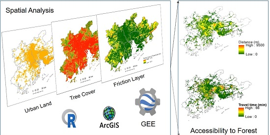
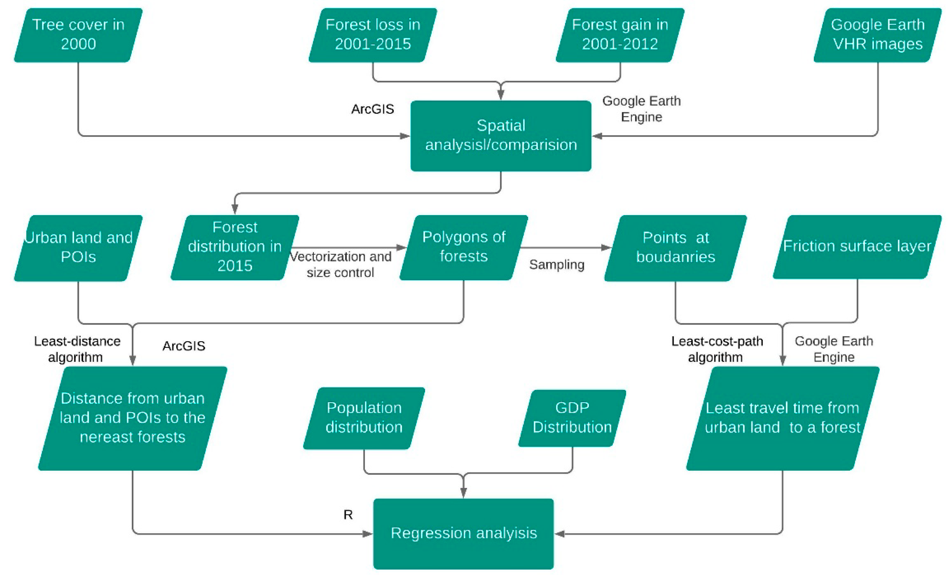
The main data analysis includes delineating the spatial distribution of >2ha forests in 2015, and then using this forest layer to compute the forest accessibility from urban land locations and POIs, quantified with both Euclidian distance and travel time. Finally, with available data on spatial distribution of population density and GDP density, regressions were applied to examine the relationship between forest accessibility and population/GDP. The major processes are demonstrated in Figure 3.

2.3.1. Forest Delineation

We derived the forest cover of the PRD for 2015 based on tree canopy cover in 2000, and forest cover gain and loss after 2000. We defined the forest cover for the year 2000 as all pixels that have tree canopy cover of >10%, which ended up being a total forest area of about 1,720,506 ha. The 10% threshold was following FAO criteria [23] but was also confirmed by visually comparing resulting forest cover with very high resolution images on Google Earth to minimize classification errors. Then, we added the locations that gained forest cover during 2000–2012 but did not lose any forest cover after 2000, and removed locations that showed only forest loss between 2000 and 2015 but no gain during 2000–2012. For locations that were observed having both forest gain and loss during the period, the decision on whether they are forest or not is depending on when the loss event has happened. Note that forest cover loss in Hansen et al. [32] was defined as a change from a forest to non-forest state, or sometimes a stand-replacement disturbance. A stand-replacement disturbance suggests that, after original trees were eliminated (forest loss), new or young trees may have been re-planted (forest gain). Therefore, if a location was observed as undergoing forest loss before 2010 but meanwhile forest gain was reported, we regarded it as remaining as a forest in 2015; if forest loss was observed after 2010 for a location, we regarded it as no longer a forest in 2015. The processes assume that there was no forest gain between 2012 and 2015 (note that there is no database on forest gain after 2012). This assumption is based on the argument that tree growth over a 3-year period is negligible. Lastly, we converted the raster forest layer to polygons and excluded all patches that were <2 ha (i.e., defining ≥ 2 ha as the effective size of forests). Using a randomly selected 600 points for validation by comparing them with Google Earth 2015 VHR images, we assessed the producer’s accuracy at 88.49% and the user’s accuracy at 89.86% for the resulting forest layer.

2.3.2. Accessibility by Distance

Distance is considered as proximity reflecting the frequency of UGS usage, i.e., people are less likely to walk to distant UGS. Distances of 300 m, 500 m, 800 m, 1000 m, 1600 m, and 2000 m have been frequently applied in the literature as an indirect estimate of walking time for measuring accessibility. In this study, we computed the distance to the closest forest patch at 30-m resolution as a measure of accessibility to forests. We then computed the proportions of land or population in the PRD urban land that have forests available within the aforementioned distances. POIs were selected to represent hotspots of human activities, with the proximity to forests from these POIs providing site-specific and category-specific information on accessibility. We therefore also computed the distance for the location of each categorized POI to its closest forest patches, and computed the percentages of POIs that have forests available within different distance thresholds at 300 m, 500 m, 800 m, 1000 m, 1600 m, and 2000 m.

2.3.3. Accessibility by Travel Time

City residents do not solely rely on walking to access UGS. Consequently, we considered multiple avenues of transportation for quantifying accessibility. We estimated the shortest travel time (the travel time with the most efficient route via an optimal combination of walking, driving, taking the bus, boats, and railways, but excluding airlines) from any pixel in the urban area to a forest patch. A least-cost-path algorithm [49], which calculates pixel-level travel time for an optimal path between any two pixels (i.e., the shortest journey time) based on the friction surface layer, was applied to each pixel in relation to all forest locations in the study area. Additionally, because the algorithm is point-based, we extracted the boundaries of each forest patch, and then sample points at these boundaries at 1-km intervals for computing travel time. The least-cost-path algorithm was then applied to compute the travel time from a pixel to each of the points located on the boundaries of all forests, with an optical path selected for the shortest travel time. We assumed that no travel time is needed from inside a forest. Therefore, we masked all pixels inside forest patches with a zero value for travel time. Note that we did not estimate travel time at resolutions of <1 km because higher resolution friction surface databases do not exist. Due to the high computational needs, the estimation of travel time was conducted using Google Earth Engine (https://code.earthengine.google.com/d1b188c4793b7cdef6836a3cbedefc89).

2.3.4. Statistical Analysis

Finally, regression was applied to investigate the relationship between distance to the nearest forest and GDP_d/POP_d, and between least travel time to a forest with GDP_d/POP_d for data extracted at 1-km resolution. Due to the large amount of pixels that may have introduced much noise into the model, the raw data were binned with a 1-min interval for travel time and a 200 m distance interval for Euclidian distance. The regression was then applied to the median value of each bin. Statistical analyses were conducted using R version 3.4.3 [50].

3. Results

3.1. Accessibility by Distance from Points of Interest

The percentages of the total number of POIs with available forests by distances from 300 to 2000 m show similar patterns among all POI types (Figure 3). Less than 20% of the POIs have access to forest patches within 300 m except for parks. There also appears a gradual increase in the percentage of POIs that have an available forest within distances from 300 to 2000 m. The percentage of total POIs with accessible forests at 1000 m increases substantially compared to shorter distances at 300-500 m, which are slightly larger than 45% for all POI types with governmental agencies and schools exceeding 50%. Within a distance of 1600–2000 m (which is about 20–30 min of walking), more than 65–75% of all of the all types of POIs have forests accessible to them. The park POIs, which provide important recreational areas for most urban residents, have better access to forests than other types of POIs at short distances (i.e., 300–500 m) but not at long distances (i.e., >1000 m) (Figure 4). Governmental agencies and schools have better accessibility (i.e., a larger proportion of the total locations with forests available) to nearby forests than other type of POIs at distances >800 m.

3.2. Accessibility from General Urban Area

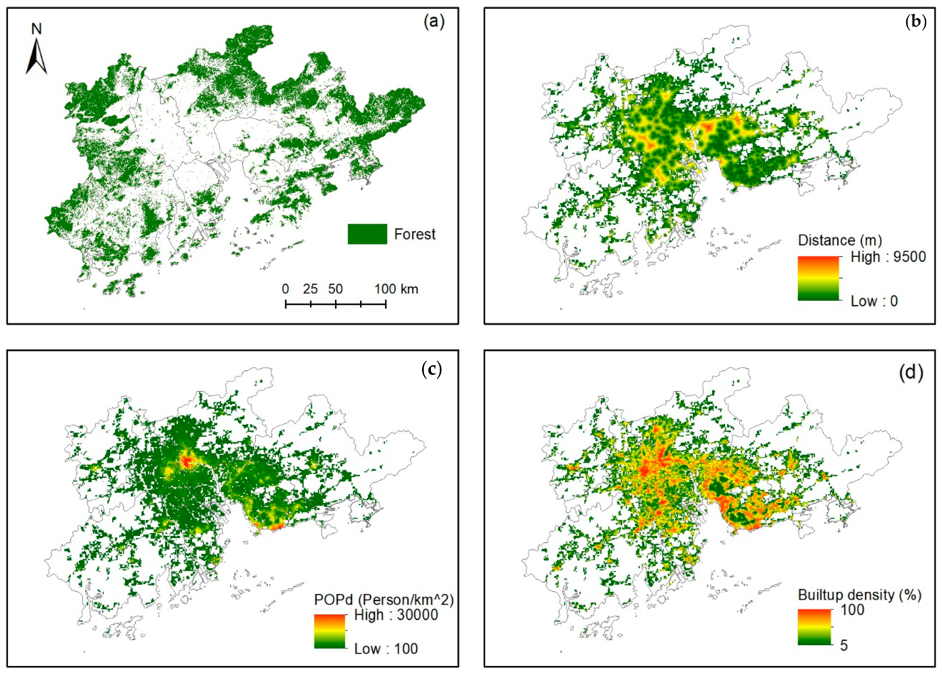
Urban land area in different locations and the corresponding populations have unequal accessibility of forests; this inequality appears to vary by distance (Figure 5). Approximately 33.9% of the total urban lands have forests within 300 m. At the distance of 1000 m, 62.4% of the total urban lands having forest patches available with this distance (which is about 14 min of walking). More than 78.5% of the total urban lands have forest patches within 1600 m. For only 7.28% of the urban land, people have to walk a straight line of >3000 m to reach a forest. From a population perspective, 20.0% of the population lives in urban areas that have forests within 300 m; 51.8% of the population has forests available within 1000 m; and 70.7% of the population has forests available within 1600 m. An interesting result is that the accumulative proportion of urban lands for any given distance is always higher than the accumulative proportion of population to access the same forest. This difference is especially pronounced at shorter distances, indicating that many urban lands closer to forests have lower population densities than those further away from a forest. The urban lands with longer distances to urban forests occur mostly in core urban areas with dense built-up cover and high population densities (Figure 6).

3.3. Travel Accessibility to Forests

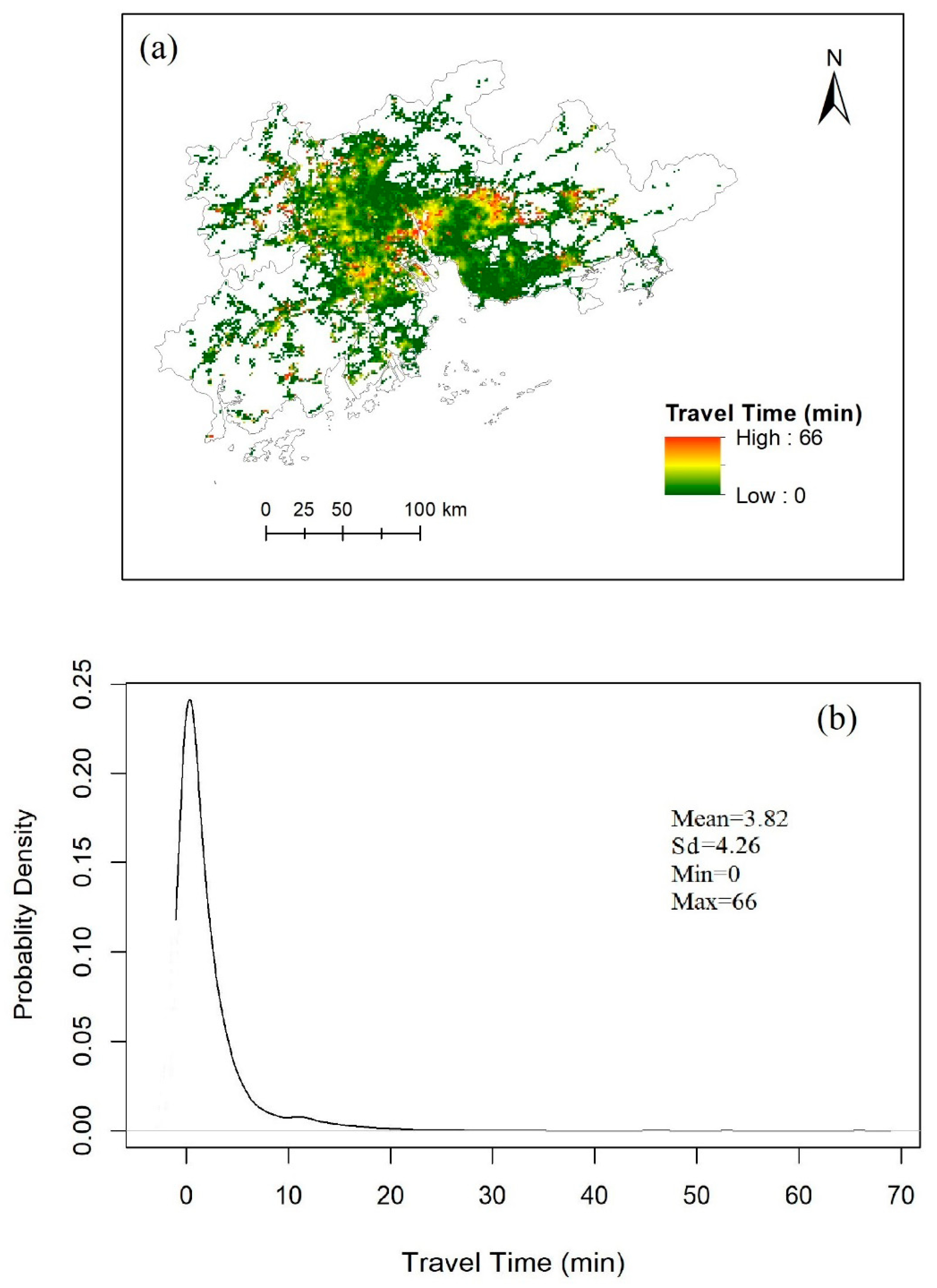
The travel time to a nearest forest patch is <15 min for most PRD urban land areas (95.6%) (Figure 7). A very small proportion (0.4%) of urban land in the PRD requires >30 min to reach a forest. For the residents, ~98% of the population lives in urban land areas with <15 min travel time to reach a forest, and only 0.6% of the population requires >30 min to access a forest. Compared to the urban centers, those living in the urban fringes require more time to travel to the closest forest.

3.4. Relationship of Accessibility with Population and Gross Domestic Product Densities

There appears a large variation in GDP_d with similar travel time to a nearest forest, with a significantly negative relationship between travel times to forests and GDP_d (Figure 8a). Throughout the PRD, more developed (i.e., higher GDP_d) areas tend to have easier access (i.e., shorter travel time) to urban forests due to multiple transport methods (vs. walking). However, if we use the straight Euclidean distance, a longer distance to the nearest forests is found for developed areas, especially when the GDP_d is low (<2+e07$/km²) (Figure 8c). Interestingly, POP_d shows no relationship with travel time. Nevertheless, POP_d and GDP_d have similar relationships with Euclidean distance to the nearest forest, i.e., a higher POPd and GDP_d is more likely to have a longer distance to the nearest forest (Figure 8d).

4. Discussion

4.1. Forests Accessibility

Our results on the distance to nearest forests show that, for a large amount of urban lands and POIs, the closest forests are >1000 m. Distance has been used as an indicator of accessibility of green space [51]. It has been reported that the use of urban green spaces (e.g., direct contact or benefit from the ecosystem services) declines with distance and increases beyond 100–300 m [52,53]. In general, the spatial proximity to green space plays an important role in human health. Reklaitiene at al. [19], for example, found a negative relationship between residential proximity to green space and depression symptoms. Having access to green spaces within 300 m was also found to be positively associated with a lower probability of high-normal blood pressure during pregnancy [20] and abnormal birth weight [54]. Mental health was also reported to decrease for residents that had access to a park within a distance of 400 m, to 800 m, 1600 m, and 3200 m [55]. Compared to the residents who live within <300 m from a green space, residents living > 1000 m away from a green space were shown to have poorer health [56].

All of these studies suggest that living in an area closer a green space is better for human health than living further away. Although no threshold has been identified or accepted from previous studies, most authors suggest a distance of less than 300–1000 m to a green space. This is in consistent with the EEA who recommends a distance of <1000 m. For the PRD, a large proportion of most urban lands (~38%) (Figure 5) and POIs (~45%) (Figure 4) are still >1000 m away from a forest, suggesting that much improvement is needed to serve urban residents. We specifically recommend that the urban designers and planners improve the availability of urban forests at closer distances. Attention is also needed for the hotspots delineated in this study for the PRD (Figure 6b), such as urban centers that lack forests within close distances. Fortunately, the travel time to the nearest forest is mostly within 15 min (Figure 7), which suggests that the urban residents can still access urban forests if they are willing to use other modes of transportation (e.g., bus, subway, or driving). In general, ~15 min is a comfortable travel time in any large urban aggregation such as the PRD. Due to the increasing competition for lands in these urban areas, an alternative policy should be made to improve the PRD’s public transportation systems.

Distance and travel time to urban forests are not independent. Together they provide a more integrated assessment for accessing forests. As aforementioned, because many ecosystem services provided by UGS (e.g., cooling, wind and flood control, and air pollution reduction) are most effective at certain short distances from the UGS [7,20,57], city residents benefit mostly from the ecosystem services provided by urban forests near to their homes. Therefore, city residents do not have to physically contact the nearby urban forests to receive their many benefits. On the other hand, for those forests that are far away from city residents, even though they could be accessed by an advanced mode of transportation in a short time, the benefits provided to visitors depends on how long the visitors can stay there. Nevertheless, for residents who do not have forests close to their homes, short travel times to distant forests become critical to take advantage of the benefits provided by forest ecosystems, such as recreational opportunities, and the positive impacts on physical and mental health. Willingness to travel to forests, however, would depend on travel time, distance, means of transportation, and the socio-demographical characteristics of the visitors [58].

4.2. Inequality of Forest Accessibility

We found large differences in forest accessibility for different urban lands and urban POIs (Figure 4, Figure 5 and Figure 6), which suggests an inequality challenge for residents living/working in these places. Policymakers need to pay additional attention to improve areas that have low accessibility. From our analysis of POIs, it appears that government agencies and schools have better accessibility to forests than other POIs (e.g., parks, residential areas, firms, hotels, and restaurants). More than half of the parks, which are important outdoor recreational sites for many Chinese residents, do not have forests available at 800–100 m distances. In China, parks are popular places used for physical exercise [59], suggesting that green spaces may play an important role in human health [55,60]. In this study, we find that the forest cover surrounding many park POIs in the PRD is not sufficient.

Given the important relationships between green space accessibility and human health, a critical question is whether access to urban forests is distributed disproportionately in an advantageous or disadvantageous manner by resident location, race, ethnicity, or income [60]. Answering this question is beyond the scope of this study because we did not have the necessary spatial data on human demography. However, we attempted to gain some insights by connecting income classes and population densities with accessibility to urban forests. In China, rich people tend to live in urban centers where GDP_d is high [61]. Therefore, it is reasonable to assume that people living in places with higher/lower GDP_d are richer/poorer groups in the PRD. In regard to the spatial proximity in Euclidean distance, people with low income were found to have forests closer to their homes (Figure 6 and Figure 8c), whereas forests were further away from the richer residents in the urban centers. These patterns are different to the findings that residents with low income had lower tree canopy cover in city neighborhoods in Indianapolis [57] and Boston [17], likely due to different stages of urbanization (i.e., urbanization versus suburbanization). Unlike previous studies that relied only on Euclidean distance, we argue that a more significant test of inequality of forest access is by examining the travel time. Our analysis suggests that richer people have a shorter travel time to forests due to more advanced transportation systems within their living landscapes (Figure 8b). Due to the fact that more people live in areas of high GDP_d, the proximity to forests has a negative relationship with population density (Figure 8d). However, while urban areas with higher population densities may have forests within a distant location, these residents have more advanced transportation tools and systems to reach forests. On the other hand, areas with lower POP_d in urban fringes may have a less developed transportation system but have forests closer by (Figure 8b). Therefore, no significant relationship is detected between travel time and population density. Regardless, inequality in accessibility to forests, which is a global phenomenon, exists within cities of the PRD. To improve the environmental good provided by urban forests, an urban planning approach with additional efforts placed on distributing green space more evenly [62], or creating more interconnected green infrastructure [63], should be promoted.

4.3. Limitations and Further Research

We presented the spatial availability in both Euclidean distance (an approximation of walking access) and travel time for accessibility of urban forests. These analyses, however, remain incomprehensive. The concept of access in reality is more complicated and requires more information beyond spatial distance and travel. For example, access to urban forests may also depend on the ownership of forests (e.g., public versus private), entrance fees and restrictions (e.g., for particular groups of people only), fencing, type and structure of the forests, etc. The access points of urban forests are also important. Not everywhere in a forest can be accessed (e.g., gated entrance). As a result, future studies may focus on forest accessibility by including access points of a forest, the physical and regulatory restrictions, entrance fees, and other information about the forests. Furthermore, some studies have shown that human demographics (e.g., gender, age, and cultural groups) may influence how people use or perceive the same green space [64,65]. Future research may gear towards the needs of different groups to evaluate green space accessibility.

Walking and traveling accessibility to urban forests are very important aspects of spatial availability. Walking availability in terms of proximity to trees or other types of green space has been widely studied in the literature, but the traveling accessibility and real walking time have not yet been fully explored. We assessed the travel time, but at a relatively coarse resolution (i.e., 1 km). As the PRD is a metropolitan area with a high population and built-up density, data with a resolution of <100 m would provide a much better profile of forest accessibility [13]. Considering that urban lands are more compact than rural areas and have complicated structure (e.g., buildings, streets, parking plot, green spot, bridges, and blocks), the walking and traveling conditions within each 1 km × 1 km pixel can be very complex. In cities, the walking time from one location to another location is much longer than taking a straight line, and the travel time may also be elongated by many unexpected factors (e.g., parking, traffic, and walkability from bus/subway stations or parking lots to the destination). For these reasons, the travel time in this study might have been underestimated. Future studies can be advanced by including data from accurate GPS navigation systems to track the travel times of public transportation, driving, walking, etc.

The estimate of distance and travel time to forests in regard to POIs, urban lands, and urban residents can also be affected by the resolutions, errors, and uncertainties associated with all input layers. For example, there are omission and commission errors for both the forest and urban land classification [42], some POIs may be missing from our data collection, and the POP_d and GDP_d have uncertainties [43,45]. These errors and uncertainties definitely affect the estimation of forest accessibility in this study but could not be quantified. Data resolution also constrains the accuracy and precision of the data, as details are hidden in a “homogeneous” pixel. We have mentioned that the travel time estimated based on the 1-km resolution friction layer may have ignored many complicated situations within a pixel and thus would have underestimated the actual value. The Euclidean distance, however, was estimated at 30 m resolution, which should have little effect on the results regarding the proximity to POIs, urban land, and urban residents at distance intervals > 100m. Nevertheless, higher resolution data from aerial photos and satellite data such as Sentinels, Landsat 8, and Worldview 3 and 4 are now available for producing more accurate land use land cover maps, and real-time navigation systems are available for accurate estimation of travel time under different travel modes. Future studies should take advantage of them for more accurate estimation of forest accessibility.

Finally, while this study focused on the PRD—a typical metropolitan area with fast urbanization—this framework could be applied to study UGS accessibility in other city clusters. Spatial distributions of urban forests and urban lands are available for many cities through national land use land cover products, or through global products such as the global forest watch program (https://www.globalforestwatch.org/), global urban footprint [66], and human settlement layers [42]. Meanwhile, POIs could be crowd-sourced from many online platforms that involve citizen science, such as such as Geo-Wiki, Open Street Maps, and Google Maps. Powered by cloud-computing engines such as Google Earth Engine, a straightforward extension can be applied to compare forest accessibility by distance and travel time, as well as their relationships with urban land and population distribution in many large city clusters globally.

5. Conclusions

We estimated the accessibility of forests to urban land and urban population in the PRD, China—a rapidly urbanizing area where forest cover has been decreasing. Accessibility was estimated from two aspects: spatial proximity to the nearest forest in Euclidean distance, and time needed to travel to the closest forest. We found that the nearest forests to a large amount of point of interests (POIs) (~450%), urban lands (~38%), and urban residents (~49%) were greater than 1000 m, suggesting a need to improve proximity to forests. There also exist insufficient forests near urban parks that are important for outdoor recreational activities for Chinese residents and visitors. The travel time to a nearby forest is generally less than 15 min for most areas (~95%) and most residents (98%), with an average travel time of 3.8 min. However, we think that the travel time may be underestimated due to limitations caused by coarse data resolution (1-km). The travel time to the closest forest is negatively correlated with GDP_d but not with POP_d. The Euclidean distance to the closest forest has a log-linear relationship with both GDP_d and POP_d. These relationships suggest inequality in forest accessibility for residents with different income levels and for areas with different population densities. Future urban planning in the PRD needs to increase not only the total coverage of forests, but also their spatial allocations for evenness.

References

- Sandström, U.G.; Angelstam, P.; Khakee, A. Urban comprehensive planning—Identifying barriers for the maintenance of functional habitat networks. Landsc. Urban Plan. 2006, 75, 43–57. [Google Scholar] [CrossRef]
- Strohbach, M.; Haase, D.; Kronenberg, J. Urban green space availability in European cities. Ecol. Indic. 2016, 70, 586–596. [Google Scholar] [CrossRef]
- Lupp, G.; Förster, B.; Kantelberg, V.; Markmann, T.; Naumann, J.; Honert, C.; Koch, M.; Pauleit, S. Assessing the recreation value of urban woodland using the ecosystem service approach in two forests in the Munich metropolitan region. Sustainability 2016, 8, 1156. [Google Scholar] [CrossRef]
- Alvey, A.A. Promoting and preserving biodiversity in the urban forest. Urban For. Urban Green. 2006, 5, 195–201. [Google Scholar] [CrossRef]
- Johnston, M.; Percival, G. Trees, people and the built environment. In Proceedings of the Urban Trees Research Conference, Birmingham, UK, 13–14 April 2011; pp. 13–14. [Google Scholar]
- Nowak, D.J.; Greenfield, E.J.; Hoehn, R.E.; Lapoint, E. Carbon storage and sequestration by trees in urban and community areas of the United States. Environ. Pollut. 2013, 178, 229–236. [Google Scholar] [CrossRef] [PubMed] [Green Version]
- Chen, J.; Zhu, L.; Fan, P.; Tian, L.; Lafortezza, R. Do green spaces affect the spatiotemporal changes of PM2.5 in Nanjing? Ecol. Process. 2016, 5, 7. [Google Scholar] [CrossRef]
- Nowak, D.J.; Crane, D.E.; Stevens, J.C. Air pollution removal by urban trees and shrubs in the United States. Urban For. Urban Green. 2006, 4, 115–123. [Google Scholar] [CrossRef] [Green Version]
- Livesley, S.J.; McPherson, G.M.; Calfapietra, C. The urban forest and ecosystem services: impacts on urban water, heat, and pollution cycles at the tree, street, and city scale. J. Environ. Qual. 2016, 45, 119. [Google Scholar] [CrossRef]
- McGrane, S.J. Impacts of urbanisation on hydrological and water quality dynamics, and urban water management: a review. Hydrol. Sci. J. 2016, 61, 2295–2311. [Google Scholar] [CrossRef] [Green Version]
- Berlin Digital Environmental Altas. Availability of Public, Near-Residential Green Space (Edition 2013). Available online: https://www.stadtentwicklung.berlin.de/umwelt/umweltatlas/eda605_01.htm (accessed on 16 July 2018).
- City of Leipzig. Umweltqualitätsziele und -standards für die Stadt Leipzig. Available online: https://www.leipzig.de/fileadmin/mediendatenbank/leipzig-de/Stadt/02.3_Dez3_Umwelt_Ordnung_Sport/36_Amt_fuer_Umweltschutz/Publikationen/Indikatoren/Umweltqualitatsziele_und-standards_fur_die_Stadt_Leipzig.pdf (accessed on 18 March 2019).
- Fan, P.; Xu, L.; Yue, W.; Chen, J. Accessibility of public urban green space in an urban periphery: The case of Shanghai. Landsc. Urban Plan. 2017, 165, 177–192. [Google Scholar] [CrossRef]
- David Stanners and Philippe Bourdeau. Europe’s Environment: The Dobris Assessment; European Environment Agency: Copenhagen, Denmark, 1995. [Google Scholar]
- World Health Organization. Urban Planning, Environment and Health: From Evidence to Policy Action; World Health Organization: Geneva, Switzerland, 2017. [Google Scholar]
- Lu, J.; Monac, M.; Newman, A.; Rae, R.A.; Campbell, L.K.; Falxa-Raymond, N.; Svendsen, E.S. MillionTreesNYC: The Integration of Research and Practice; New York City Department of Parks & Recreation: New York, NY, USA, 2014. [Google Scholar]
- Danford, R.S.; Cheng, C.; Strohbach, M.W.; Ryan, R.; Nicolson, C.; Warren, P.S. What does it take to achieve equitable urban tree canopy distribution? A boston case study. Cities Environ. 2014, 7, 2. [Google Scholar]
- Khalil, R. Quantitative evaluation of distribution and accessibility of urban green spaces (Case study: City of Jeddah). Int. J. GEOMATICS Geosci. 2014, 4, 526–535. [Google Scholar]
- Reklaitiene, R.; Grazuleviciene, R.; Dedele, A.; Virviciute, D.; Vensloviene, J.; Tamosiunas, A.; Baceviciene, M.; Luksiene, D.; Sapranaviciute-Zabazlajeva, L.; Radisauskas, R.; et al. The relationship of green space, depressive symptoms and perceived general health in urban population. Scand. J. Public Health 2014, 42, 669–676. [Google Scholar] [CrossRef]
- Grazuleviciene, R.; Dedele, A.; Danileviciute, A.; Vencloviene, J.; Grazulevicius, T.; Andrusaityte, S.; Uzdanaviciute, I.; Nieuwenhuijsen, M.J. The influence of proximity to city parks on blood pressure in early pregnancy. Int. J. Environ. Res. Public Health 2014, 11, 2958–2972. [Google Scholar] [CrossRef] [PubMed]
- Moore, L.V.; Diez Roux, A.V.; Evenson, K.R.; McGinn, A.P.; Brines, S.J. Availability of recreational resources in minority and low socioeconomic status areas. Am. J. Prev. Med. 2008, 34, 16–22. [Google Scholar] [CrossRef]
- Maroko, A.R.; Maantay, J.A.; Sohler, N.L.; Grady, K.L.; Arno, P.S. The complexities of measuring access to parks and physical activity sites in New York City: a quantitative and qualitative approach. Int. J. Health Geogr. 2009, 8, 34. [Google Scholar] [CrossRef]
- FAO. FRA 2000 on Definitions of Forest and Forest Change; FAO: Rome, Italy, 2000. [Google Scholar]
- Barbosa, O.; Tratalos, J.A.; Armsworth, P.R.; Davies, R.G.; Fuller, R.A.; Johnson, P.; Gaston, K.J. Who benefits from access to green space? A case study from Sheffield, UK. Landsc. Urban Plan. 2007, 83, 187–195. [Google Scholar] [CrossRef]
- Weiss, D.J.; Nelson, A.; Gibson, H.S.; Temperley, W.; Peedell, S.; Lieber, A.; Hancher, M.; Poyart, E.; Belchior, S.; Fullman, N.; et al. A global map of travel time to cities to assess inequalities in accessibility in 2015. Nature 2018, 553, 333–336. [Google Scholar] [CrossRef]
- Žlender, V.; Ward Thompson, C. Accessibility and use of peri-urban green space for inner-city dwellers: A comparative study. Landsc. Urban Plan. 2017. [Google Scholar] [CrossRef]
- Yu, W.; Zhou, W. The spatiotemporal pattern of urban expansion in China: A comparison study of three urban megaregions. Remote Sens. 2017, 9, 45. [Google Scholar] [CrossRef]
- Zhang, Q.; Seto, K.C. Mapping urbanization dynamics at regional and global scales using multi-temporal DMSP/OLS nighttime light data. Remote Sens. Environ. 2011, 115, 2320–2329. [Google Scholar] [CrossRef]
- Lu, X.; Fung, J.C.H.; Wu, D. Modeling wet deposition of acid substances over the PRD region in China. Atmos. Environ. 2015, 122, 819–828. [Google Scholar] [CrossRef]
- Zhang, Y.; Wang, Y.; Wang, Y.; Xi, H. Investigating the impacts of landuse-landcover (LULC) change in the Pearl River Delta region on water quality in the Pearl River estuary and Hong Kong’s coast. Remote Sens. 2009, 1, 1055–1064. [Google Scholar] [CrossRef]
- Li, L.; Yang, J.; Wang, Y. Retrieval of high-resolution atmospheric particulate matter concentrations from satellite-based aerosol optical thickness over the Pearl River Delta area, China. Remote Sens. 2015, 7, 7914–7937. [Google Scholar] [CrossRef]
- Hansen, M.C.; Potapov, P.V.; Moore, R.; Hancher, M.; Turubanova, S.A.; Tyukavina, A.; Thau, D.; Stehman, S.V.; Goetz, S.J.; Loveland, T.R.; et al. High-resolution global maps of 21st-century forest cover change. Science 2013, 342, 850–853. [Google Scholar] [CrossRef]
- Gong, C.; Yu, S.; Joesting, H.; Chen, J. Determining socioeconomic drivers of urban forest fragmentation with historical remote sensing images. Landsc. Urban Plan. 2013. [Google Scholar] [CrossRef]
- Tian, L.; Chen, J.; Yu, S.X. Coupled dynamics of urban landscape pattern and socioeconomic drivers in Shenzhen, China. Landsc. Ecol. 2014. [Google Scholar] [CrossRef]
- The World Bank. World Bank Report Provides New Data to Help Ensure Urban Growth Benefits the Poor. Available online: http://www.worldbank.org/en/news/press-release/2015/01/26/world-bank-report-provides-new-data-to-help-ensure-urban-growth-benefits-the-poor (accessed on 17 July 2018).
- Shen, J. Urbanization, Regional Development and Governance in China; Routledge: Abingdon-on-Thames, UK, 2018; ISBN 9781315143255. [Google Scholar]
- Tyrväinen, L.; Pauleit, S.; Seeland, K.; De Vries, S. Benefits and uses of urban forests and trees. In Urban Forests and Trees: A Reference Book; Springer: Berlin/Heidelberg, Germany, 2005; ISBN 354025126X. [Google Scholar]
- Miller, J. Examining the Hansen Global Forest Change (2000–2014) Dataset within an Australian Local Government Area; University of Southern Queensland: Toowoomba, Australia, 2016. [Google Scholar]
- Brodersen, K.H.; Ong, C.S.; Stephan, K.E.; Buhmann, J.M. The balanced accuracy and its posterior distribution. In Proceedings of the 2010 20th International Conference on Pattern Recognition, Istanbul, Turkey, 23–26 August 2010; IEEE: Piscataway, NJ, USA, 2010; pp. 3121–3124. [Google Scholar]
- Florczyk, A.J.; Pesaresi, M.; Ehrlich, D.; Ferri, S.; Syrris, V.; Soille, P.; Kemper, T.; Julea, A.; Halkia, M.; Freire, S.; et al. Operating Procedure for the Production of the Global Human Settlement Layer from Landsat Data of the Epochs 1975, 1990, 2000, and 2014; Joint Research Center: Brussels, Belgium, 2016. [Google Scholar]
- Klotz, M.; Kemper, T.; Geiß, C.; Esch, T.; Taubenböck, H. How good is the map? A multi-scale cross-comparison framework for global settlement layers: Evidence from Central Europe. Remote Sens. Environ. 2016, 178, 191–212. [Google Scholar] [CrossRef] [Green Version]
- Pesaresi, M.; Freire, S. GHS Settlement Grid, Following the REGIO Model 2014 in Application to GHSL Landsat and CIESIN GPW v4-Multitemporal (1975-1990-2000-2015); Joint Research Center: Brussels, Belgium, 2016. [Google Scholar]
- Doxsey-Whitfield, E.; MacManus, K.; Adamo, S.B.; Pistolesi, L.; Squires, J.; Borkovska, O.; Baptista, S.R. Taking advantage of the improved availability of census data: A first look at the gridded population of the World, version 4. Pap. Appl. Geogr. 2015, 1, 226–234. [Google Scholar] [CrossRef]
- Bai, Z.; Wang, J.; Wang, M.; Gao, M.; Sun, J. Accuracy assessment of multi-source gridded population distribution datasets in China. Sustainability 2018, 10, 1363. [Google Scholar] [CrossRef]
- Kummu, M.; Taka, M.; Guillaume, J.H.A. Gridded global datasets for Gross Domestic Product and Human Development Index over 1990–2015. Sci. Data 2018, 5, 180004. [Google Scholar] [CrossRef] [Green Version]
- Cai, J.; Huang, B.; Song, Y. Using multi-source geospatial big data to identify the structure of polycentric cities. Remote Sens. Environ. 2017, 202, 210–221. [Google Scholar] [CrossRef]
- Yao, Y.; Liu, X.; Li, X.; Zhang, J.; Liang, Z.; Mai, K.; Zhang, Y. Mapping fine-scale population distributions at the building level by integrating multisource geospatial big data. Int. J. Geogr. Inf. Sci. 2017, 1–25. [Google Scholar] [CrossRef]
- Ye, T.; Zhao, N.; Yang, X.; Ouyang, Z.; Liu, X.; Chen, Q.; Hu, K.; Yue, W.; Qi, J.; Li, Z.; Jia, P. Improved population mapping for China using remotely sensed and points-of-interest data within a random forests model. Sci. Total Environ. 2019, 658, 936–946. [Google Scholar] [CrossRef] [PubMed]
- Dijkstra, E.W. A note on two problems in connexion with graphs. Numer. Math. 1959, 1, 269–271. [Google Scholar] [CrossRef] [Green Version]
- R Core Team. R: A Language and Environment for Statistical Computing; R Foundation for Statistical Computing: Vienna, Austria, 2013. [Google Scholar]
- Ekkel, E.D.; de Vries, S. Nearby green space and human health: Evaluating accessibility metrics. Landsc. Urban Plan. 2017, 157, 214–220. [Google Scholar] [CrossRef]
- Nielsen, T.S.; Hansen, K.B. Do green areas affect health? Results from a Danish survey on the use of green areas and health indicators. Health Place 2007, 13, 839–850. [Google Scholar] [CrossRef]
- Grahn, P.; Stigsdotter, U.A. Landscape planning and stress. Urban For. Urban Green. 2003, 2, 1–18. [Google Scholar] [CrossRef]
- Dadvand, P.; Wright, J.; Martinez, D.; Basagaña, X.; McEachan, R.R.C.; Cirach, M.; Gidlow, C.J.; de Hoogh, K.; Gražulevičiene, R.; Nieuwenhuijsen, M.J. Inequality, green spaces, and pregnant women: Roles of ethnicity and individual and neighbourhood socioeconomic status. Environ. Int. 2014, 71, 101–108. [Google Scholar] [CrossRef] [PubMed]
- Sturm, R.; Cohen, D. Proximity to urban parks and mental health. J. Ment. Health Policy Econ. 2014, 17. [Google Scholar] [CrossRef]
- Stigsdotter, U.K.; Ekholm, O.; Schipperijn, J.; Toftager, M.; Kamper-Jørgensen, F.; Randrup, T.B. Health promoting outdoor environments - Associations between green space, and health, health-related quality of life and stress based on a Danish national representative survey. Scand. J. Public Health 2010, 38, 411–417. [Google Scholar] [CrossRef] [PubMed]
- Hauru, K.; Eskelinen, H.; Yli-Pelkonen, V.; Kuoppamäki, K.; Setälä, H. Residents’ perceived benefits and the use of urban nearby forests. Int. J. Appl. For. 2015, 2, 1–23. [Google Scholar] [CrossRef]
- Rossi, S.D.; Byrne, J.A.; Pickering, C.M. The role of distance in peri-urban national park use: Who visits them and how far do they travel? Appl. Geogr. 2015. [Google Scholar] [CrossRef]
- Giles-Corti, B.; Macintyre, S.; Clarkson, J.P.; Pikora, T.; Donovan, R.J. Environmental and lifestyle factors associated with overweight and obesity in Perth, Australia. Am. J. Heal. Promot. 2003, 18, 93–102. [Google Scholar] [CrossRef] [PubMed]
- Wolch, J.R.; Byrne, J.; Newell, J.P. Urban green space, public health, and environmental justice: The challenge of making cities “just green enough”. Landsc. Urban Plan. 2014, 125, 234–244. [Google Scholar] [CrossRef]
- Gu, C.; Wu, L.; Cook, I. Progress in research on Chinese urbanization. Front. Archit. Res. 2012. [Google Scholar] [CrossRef]
- Yao, L.; Liu, J.; Wang, R.; Yin, K.; Han, B. Effective green equivalent—A measure of public green spaces for cities. Ecol. Indic. 2014, 47, 123–127. [Google Scholar] [CrossRef] [Green Version]
- Lafortezza, R.; Davies, C.; Sanesi, G.; Konijnendijk, C.C. Green infrastructure as a tool to support spatial planning in European urban regions. IForest 2013, 6, 102–108. [Google Scholar] [CrossRef]
- Gungor, B.S.; Chen, J.; Wu, S.R.; Zhou, P.; Shirkey, G. Does plant knowledge within urban forests and parks directly influence visitor pro-environmental behaviors. Forests 2018, 9, 171. [Google Scholar] [CrossRef]
- Zheng, B.; Zhang, Y.; Chen, J. Preference to home landscape: Wildness or neatness? Landsc. Urban Plan. 2011. [Google Scholar] [CrossRef]
- Esch, T.; Marconcini, M.; Felbier, A.; Roth, A.; Heldens, W.; Huber, M.; Schwinger, M.; Taubenbock, H.; Muller, A.; Dech, S. Urban footprint processor-Fully automated processing chain generating settlement masks from global data of the TanDEM-X mission. IEEE Geosci. Remote Sens. Lett. 2013. [Google Scholar] [CrossRef]
Figure 1.
Forest loss in the Pearl River Delta (PRD) from 2001 through 2016, as percentages of total forest area in 2000, which is about 1,720,506 ha. The forest loss was computed based on Hansen et al.’s forest loss layers at 30-m resolution [32] through zonal statistics analysis in Google Earth Engine.
Figure 2.
Location of the Pearl River Delta (PRD) economic zone in southern China. Hong Kong and Macao are also broadly defined as parts of the greater PRD but are excluded in this study because of different governances.
Figure 3.
A flowchart that demonstrates the main processes in this study used to estimate the forest accessibility by using both distance and travel time. POIs: points of interest; GDP: gross domestic product; VHR: very high resolution.
Figure 4.
Proportion (%) of the total number of Points of Interest (POI) that have forests accessible at distances of 300 m, 500 m, 800 m, 1000 m, 1600 m, and 2000 m. The POI type is labeled on top of each panel.
Figure 5.
The changes in the accumulated proportion of urban land areas (%) and the corresponding population (%) that have forests available with fixed distances. Note: due to data resolution (30-m for forest cover), the statistics were computed at 100 m intervals, with a starting distance of 300 m.
Figure 6.
The spatial distribution of forests (a), Euclidean straight distance to the closest forest (b), population density (POPd) (c), and built-up density (d) in the Pearl River Delta (PRD).
Figure 7.
The travel time to the nearest forest (a) and the accompanying probability density distribution (b).
Figure 8.
The linear relationship between GDP density (GDPd) and (a) population density (POPd) (b) travel time to the nearest forest; and the log-linear relationship between GDPd and (c) POPd (d) the Euclidian distance to the closest forests. Data are grouped with a 1-min interval for travel time and 200 m for Euclidian distance. The black dots represent the median value from each group while the gray bars show the 10% and 90% quantiles. The regression analysis is performed with median values.
© 2019 by the authors. Licensee MDPI, Basel, Switzerland. This article is an open access article distributed under the terms and conditions of the Creative Commons Attribution (CC BY) license (http://creativecommons.org/licenses/by/4.0/).
Share and Cite
MDPI and ACS Style
Zhang, R.; Chen, J.; Park, H.; Zhou, X.; Yang, X.; Fan, P.; Shao, C.; Ouyang, Z. Spatial Accessibility of Urban Forests in the Pearl River Delta (PRD), China. Remote Sens. 2019, 11, 667. https://doi.org/10.3390/rs11060667
AMA Style
Zhang R, Chen J, Park H, Zhou X, Yang X, Fan P, Shao C, Ouyang Z. Spatial Accessibility of Urban Forests in the Pearl River Delta (PRD), China. Remote Sensing. 2019; 11(6):667. https://doi.org/10.3390/rs11060667
Chicago/Turabian StyleZhang, Rong, Jiquan Chen, Hogeun Park, Xuhui Zhou, Xuchao Yang, Peilei Fan, Changliang Shao, and Zutao Ouyang. 2019. "Spatial Accessibility of Urban Forests in the Pearl River Delta (PRD), China" Remote Sensing 11, no. 6: 667. https://doi.org/10.3390/rs11060667
Note that from the first issue of 2016, this journal uses article numbers instead of page numbers. See further details here.