Article

A Novel Tri-Training Technique for the Semi-Supervised Classification of Hyperspectral Images Based on Regularized Local Discriminant Embedding Feature Extraction

1
Key Laboratory for Land Environment and Disaster Monitoring of NASG, China University of Mining and Technology, Xuzhou 221116, China
2
Key Laboratory of Geographic Information Science (Ministry of Education), East China Normal University, Shanghai 200241, China
3
Department of Electrical and Computer Engineering, Mississippi State University, Starkville, MS 39762, USA
4
Chang Guang Satellite Technology Co. Ltd., Changchun 130033, China
*
Authors to whom correspondence should be addressed.
Remote Sens. 2019, 11(6), 654; https://doi.org/10.3390/rs11060654
Submission received: 1 February 2019 / Revised: 12 March 2019 / Accepted: 15 March 2019 / Published: 18 March 2019

Abstract

:
This paper introduces a novel semi-supervised tri-training classification algorithm based on regularized local discriminant embedding (RLDE) for hyperspectral imagery. In this algorithm, the RLDE method is used for optimal feature information extraction, to solve the problems of singular values and over-fitting, which are the main problems in the local discriminant embedding (LDE) and local Fisher discriminant analysis (LFDA) methods. An active learning method is then used to select the most useful and informative samples from the candidate set. In the experiments undertaken in this study, the three base classifiers were multinomial logistic regression (MLR), k-nearest neighbor (KNN), and random forest (RF). To confirm the effectiveness of the proposed RLDE method, experiments were conducted on two real hyperspectral datasets (Airborne Visible/Infrared Imaging Spectrometer (AVIRIS) and Reflective Optics System Imaging Spectrometer (ROSIS)), and the proposed RLDE tri-training algorithm was compared with its counterparts of tri-training alone, LDE, and LFDA. The experiments confirmed that the proposed approach can effectively improve the classification accuracy for hyperspectral imagery.

1. Introduction

Hyperspectral sensors have hundreds of spectrally contiguous bands, which can provide abundant spectral information [1]. Due to the high spectral resolution, hyperspectral images (HSIs) have been widely used in applications such as agricultural mapping [2], water quality analysis [3], and mineral identification [4]. The key component in these applications is the classification. Some of the conventional supervised classifiers can offer satisfactory classification performances, but the performance is dependent on both the quantity and quality of the training samples. However, labeled training samples can be costly, difficult, and time-consuming to obtain, and it is difficult for the traditional supervised classifiers to obtain good performances when the number of labeled training samples is limited [5]. Despite the fact that deep learning based methods have now been developed for HSI classification, including convolutional neural networks (CNNs) [6,7,8], 3D convolutional neural networks (3D-CNNs) [9,10], and long short-term memory (LSTM) networks [11,12], these problems still exist. Therefore, how to use unlabeled samples to improve the classification performance has become a hot research topic. The use of unlabeled samples to improve the classification performance is known as semi-supervised learning [13]. Common semi-supervised learning algorithms include multi-view learning algorithms [14], self-learning algorithms [15], tri-training algorithms [16], graph-based approaches [17], and the transductive support vector machine (TSVM) algorithm [18]. High-dimensional data processing needs more storage and computation time [19,20]. In addition, the spectral bands in an HSI are highly correlated, and the classification performance deteriorates as the dimensionality increases (the Hughes phenomenon) with limited training samples [21,22]. Therefore, in order to reduce the time consumption and improve the classification performance, it is necessary to extract the useful spectral information before performing classification.
The basic technique of spectral information extraction is dimension reduction, the goal of which is to embed the high-dimensional data in a low-dimensional space containing the crucial information [23,24]. Research into dimension reduction has experienced rapid development in recent years. Linear dimension reduction methods obtain the spectral information in the low-dimensional space by building a linear model. Typical methods include principal component analysis (PCA) [25], linear discriminant analysis (LDA) [26], direct linear discriminant analysis (DLDA) [27], and the maximum margin criterion (MMC) [28]. These methods are simple to operate, efficient, and have a strong generalization ability for linear datasets. However, these methods cannot obtain satisfactory performances in nonlinear datasets. Therefore, nonlinear dimension reduction methods have been proposed for use with nonlinear datasets [29]. Common nonlinear dimension reduction methods include kernel based approaches [30,31] and manifold learning algorithms [32]. In [33], kernel PCA was first proposed to solve the sparsity and dimensionality problems of nonlinear datasets. In [34], a new nonlinear dimension reduction method combining a kernel function with Fisher discriminant analysis was used in the classification of HSIs. In [35,36], Song et al. proposed models to learn a set of robust hash functions to map the high-dimensional data points into binary hash codes by effectively utilizing the local structural information. However, how to select a suitable kernel function lacks a theoretical basis.
The manifold learning algorithms depict the intrinsic structure of high-dimensional data by constructing a representation of the data lying in a low-dimensional manifold [31]. Tenenbaum [37] tried to preserve the geodesic distances based on multi-dimensional scaling, and proposed the isometric feature mapping (Isomap) method. In [38], locally linear embedding (LLE) was used to embed data points in a low-dimensional space by finding the optimal linear reconstruction in a small neighborhood. He et al. [39] subsequently proposed the neighborhood preserving embedding algorithm based on LLE, and regarded the error minimization as the objective function. In [40], the local discriminant embedding (LDE) algorithm was used to extend global LDA to a local version, so as to perform the local discriminant embedding in a graph embedding framework. However, the aforementioned manifold learning algorithms have singularity and cannot preserve the data diversity in the case of limited training samples.
Therefore, in this paper, we propose a new feature extraction method—regularized local discriminant embedding (RLDE)—to preserve the local feature information and overcome the singularity when training samples are limited. In order to make full use of the unlabeled samples, we select the semi-supervised tri-training algorithm. We also use an active learning method to select the unlabeled samples and use ensemble learning to improve the classification result.

2. Spatial Mean Filtering and Feature Extraction

X = [ x 1 , x 2 , , x m ] R n × m denotes the training dataset with n-dimensional feature vectors; Y = [ y 1 , y 2 , , y m ] R represents the corresponding labels; m is the number of training samples; and all the datasets are denoted as { x i } i = 1 l R n , where l is the number of datasets.

2.1. Spatial Mean Filtering

To reduce noise and smooth the homogeneous regions, we first use spatial mean filtering to preprocess the HSIs. The spatial mean filtering of a labeled pixel X i is denoted as:
X i =   X i +   k = 1 w 2 1 v k X i k 1 + k = 1 w 2 1 v k ,
where w is the width of the neighborhood window; s = w 2 1 is the number of neighbors of X i ; v k = exp { γ 0 | | X i X i k | | 2 } stands for the spectral distance of the neighboring pixels to the central pixel; and γ 0 represents the degree of filtering.

2.2. Local Discriminant Embedding (LDE)

LDE is a nonlinear supervised dimension reduction method. The local information of homogeneous and heterogeneous samples is preserved by defining inter-class graphs and within-class graphs [41,42]. The basic idea is to simultaneously attain between-class separation and within-class local structure preservation. The objective function of LDE is denoted as:
{ J ( V ) = a r g m a x i , j V T x i V T x j 2 ω i , j s . t . i , j V T x i V T x j 2 ω i , j = 1 ,
where V is the optimal projection matrix; and ω , ω are the weight matrix of the heterogeneous neighboring sample points and the weight matrix of the nearest-neighbor sample points, which are defined as:
ω i , j = { e x p [ x i x j 2 / t ]   i f   x i N ( x j )   o r   x j N ( x i )                                 a n d   y x i y x j 0                               o t h e r w i s e ,
ω i , j = { e x p [ x i x j 2 / t ]   i f   x i N ( x j )   o r   x j N ( x i )                                 a n d   y x i = y x j 0                               o t h e r w i s e ,
where t is a constant parameter, and the value of t is the square of the mean value of the Euclidean distances between the sample points. N ( x ) is the k neighborhood samples of training sample x .
Equation (2) can be converted into:
J = i , j t r { V T ( x i x j ) ( x i x j ) T V } ω i , j .
After conversion, we can obtain:
J = 2 t r { V T X ( D W ) X T V } .
Thus, the objective function can be written as follows:
{ J ( V ) = 2 t r { V T X ( D W ) X T V } s . t .   2 t r { V T X ( D W ) X T V } = 1 ,
where D and D are diagonal matrices, and the diagonal elements are D i , i = ω i , j and D i , i = ω i , j . W and W are affinity weight matrices, which are sparse and symmetric, as computed by Equations (3) and (4), respectively.
The optimal LDE projection is obtained by finding the eigenvectors corresponding to nonzero small eigenvalues of the following generalized Eigen-decomposition problem:
X (   D     W   ) X T V = λ X ( D W ) X T V .

2.3. Regularized Local Discriminant Embedding (RLDE)

The manifold structure of all the data can be obtained after simulating the manifold structure of the training data through the LDE and local Fisher discriminant analysis (LFDA) algorithms [43,44]. These algorithms can not only detect the internal structure, but can also preserve the discriminative structure of the data [45]. However, the LDE and LFDA algorithms have the following shortcomings: (1) when the number of training samples is smaller than the spectral dimension, the singular value problem occurs in the process of solving the projection vector and (2) in attempting to preserve the local difference information, the over-fitting problem occurs [46]. Therefore, we propose the RLDE method to solve the above problems. The objective function of this method is derived from Equation (2):
J ( V ) = { a r g m a x { α i , j V T X i V T X j 2 ω i , j i , j V T X i V T X j 2 ω i , j + ( 1 α ) R r e g f ( x ) } s . t .   V V T = 1 ,
where
R r e g f ( x ) = i , j V T X i V T X j 2 i , j V T X i V T X j 2 ω i , j
is the added regular constraint, and α is a regularization parameter with a value of [0,1]. Equation (10) is equivalent to:
{ J ( V ) = a r g m a x { 2 t r { α V T X ( D W ) X T V + ( 1 α ) V T X X T V } / 2 t r { α V T X ( D W ) X T V + ( 1 α ) d i a g ( V T X ( D W ) X T V ) X X T } } s . t .   V V T = 1 .
The optimized objective of LDE is to maximize i , j V T X i V T X j 2 ω i , j and minimize i , j V T X i V T X j 2 ω i , j , where X X T is utilized to preserve the maximal data variance. The diagonal regularization in the denominator improves the stability of the solution, without impacting the local intra-class neighborhood preserving ability. RLDE is suitable for the small-sample-size HSI classification problem. The item V T X ( D W ) X T V is used to maintain the intra-class relationships. The item X X T is used to keep the maximal data variance.
The optimal RLDE projection is obtained by finding the eigenvectors corresponding to nonzero small eigenvalues of the following generalized Eigen-decomposition problem:
( α X ( D W ) X T + ( 1 α ) X X T ) V = λ ( α ( X ( D W ) X T ) + ( 1 α ) ( d i a g ( X ( D W ) X T ) ) ) V .

2.4. Cooperative Training Strategy Combining Local Features

In [47], the optimal classifier combination selected by the diversity measures was multinomial logistic regression (MLR), k-nearest neighbor (KNN), and extreme learning machine (ELM). In this study, the correlation coefficient, disagreement metric, and double-fault measure were implemented to select the optimal classifier combination. It was found that the combination of MLR, KNN, and random forest (RF) achieved the best performance. Hence, the base classifiers were selected as MLR, KNN, and RF in this research. The procedure of the proposed method can be summarized as follows.
(1)
A mean filtering process is employed to reduce the noise in the HSI.
(2)
The local feature information of training samples L i is extracted by the RLDE method, and is labeled L i .
(3)
The classifier h i is trained with L i , to obtain the predicted classification result S i .
(4)
For the classifier h i , another two classifiers are selected which agree on the labeling of these samples to build the candidate set U i .
(5)
The active learning method is used to select the most useful and informative samples L i from the candidate sets L i = L i L i and U i = U i U i .
(6)
The process is terminated if the stopping condition is met; otherwise, go to Step (2).
The final classification result is obtained by the majority voting method.
Pseudo-code Describing the RLDE Tri-Training Algorithm
Algorithm: RLDE tri-training
Input: L: Original labeled sample set
   U: Unlabeled sample set
   BT: Breaking ties algorithm
   MV: Majority voting algorithm
Process:
   L←SMF(L); U←SMF(U)
   L1L; L2L; L3L
   Repeat until none of hi(i∈{1,2,3}) changes
      L 1 ←RLDE( L 1 ); L 2 ←RLDE( L 2 ); L 3 ←RLDE( L 3 )
      h 1 MLR( L 1 ); h 2 KNN( L 2 ); h 1 RF( L 3 )
      S 1 h 1 ( U 1 ) ; S 2 h 2 ( U 2 ) ; S 3 h 3 ( U 3 )
     For i ∈ {1,2,3} do
       S i S j S k (i ≠ j ≠ k)
       L i ←BT( S i )
       L i L i L i ; U i ( U i L i )
     End of for
   End of repeat
OUTPUT: S MV( S 1 + S 2 + S 3 )

3. Experimental Results and Analysis

In the spatial mean filtering (SMF) operation, the parameters for the Airborne Visible/Infrared Imaging Spectrometer (AVIRIS) dataset were set as follows: the degree of filtering   γ 0 = 0.9 and the filtering window w = 9. The parameters for the Reflective Optics System Imaging Spectrometer (ROSIS) dataset were set as γ 0 = 0.9 and w = 7. These parameters can prevent over-filtering and increase the similarity and consistency of the neighboring pixels. In the feature extraction, the parameter in RLDE was selected as α = 0.5 for the AVIRIS dataset and 0.7 for the ROSIS dataset. We selected L = 5, 10, and 15 samples per class as the initial labeled training sets. We set k = 3 for KNN, and the parameter settings of MLR and RF were set as the default values. The number of most useful and informative samples in each iteration was set as 100. All the experiments were carried out 10 times, and the average results are reported. The initial training samples also have an impact on the accuracy (see Section 4). The experiments were therefore performed with the optimal feature number for each dataset.

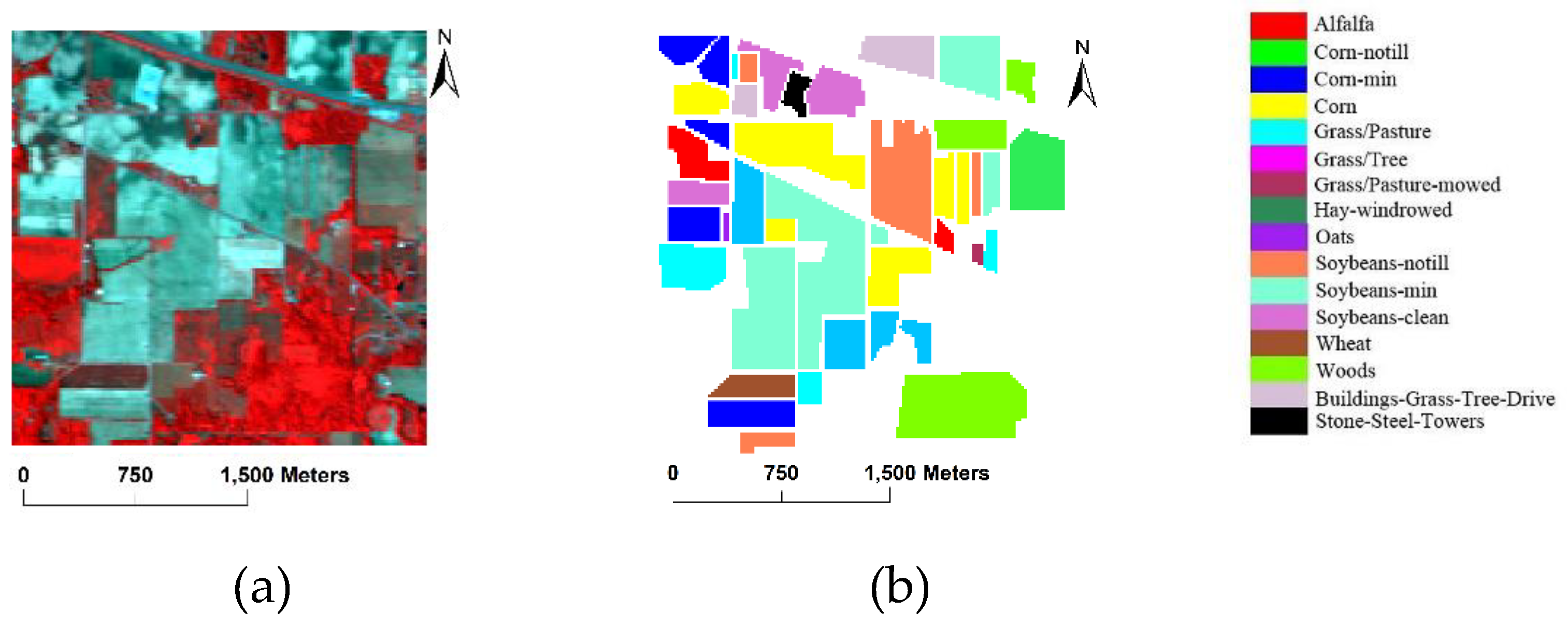
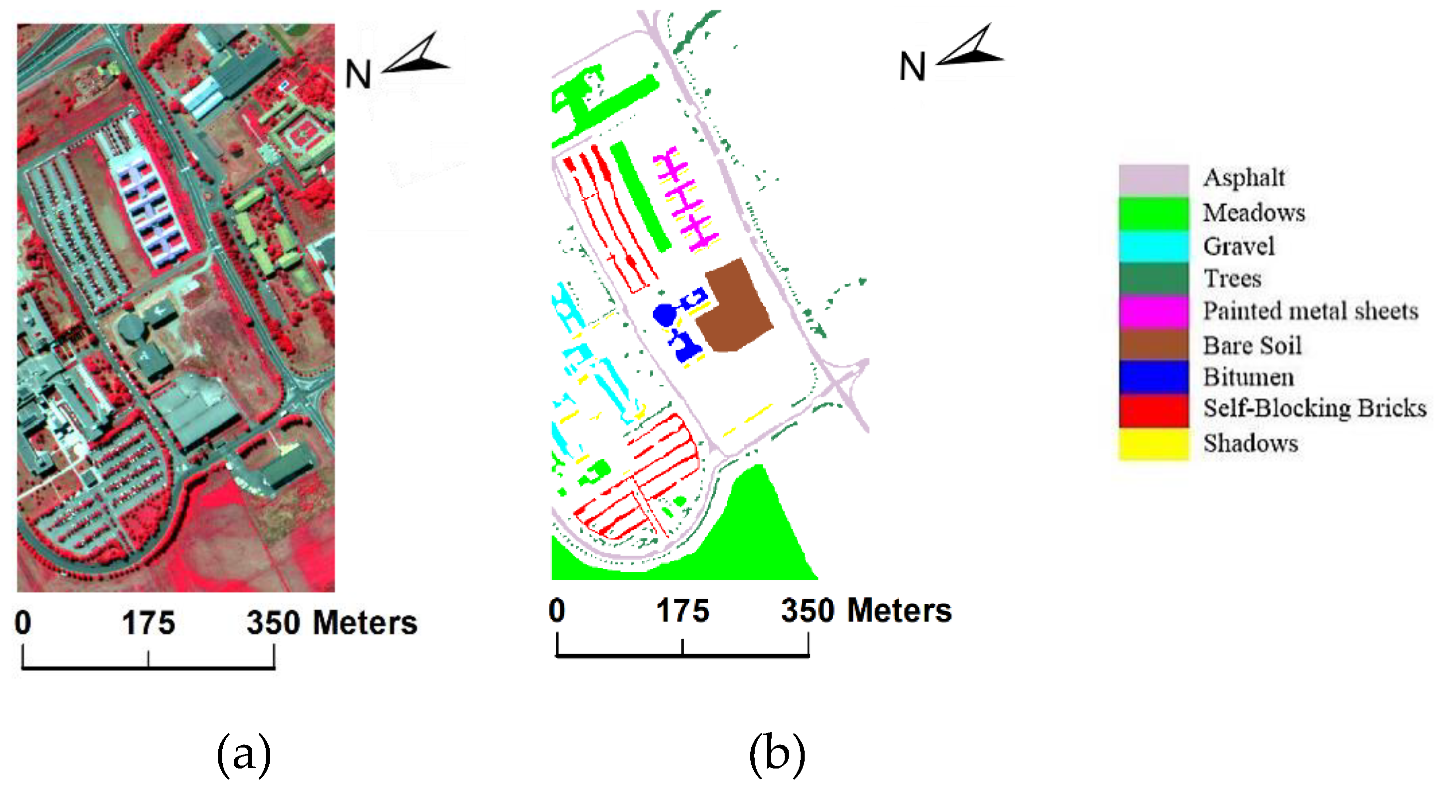
3.1. Data Used in the Experiments

In the experiments, two real HSIs were used to evaluate the proposed approach. The HSI used in the first experiment was collected by the AVIRIS sensor over the Indian Pines test site in Northwestern Indiana in 1992. This dataset has a spatial size of 145 × 145 pixels and is made up of 224 spectral bands in the wavelength range of 0.4–2.5 um at 10 nm intervals, with a spatial resolution of 20 m. In total, 202 bands were used in the experiment after the noisy and water absorption bands were removed. For illustrative purposes, the image scene in pseudocolor is shown in Figure 1a. The ground-truth map available for the scene with 16 mutually exclusive ground-truth classes is shown in Figure 1b.
The HSI used in the second experiment was collected by the ROSIS sensor over the urban area of the University of Pavia, Italy. This dataset has a spatial size of 610 × 340 pixels and is made up of 115 spectral bands in the wavelength range of 0.43–0.68 um, with a spatial resolution of 1.3 m. In total, 103 bands were used in the experiment after the noisy and water absorption bands were removed. For illustrative purposes, the image scene in pseudocolor is shown in Figure 2a. The ground-truth map available for the scene with nine mutually exclusive ground-truth classes is shown in Figure 2b.

3.2. The Effect of the Spatial Mean Filtering

Table 1 and Figure 3 show the classification results of the tri-training algorithm based on the RLDE method, using spatial mean filtering (SMF) and non-spatial mean filtering (non-SMF). As the unlabeled samples are continuously added, the classification accuracy increases. However, when the iterations reach seven, the classification accuracy starts to level off. In the AVIRIS experiment, with 5, 10, and 15 initial training samples per class, the overall accuracy (OA) of SMF increases by 12.19%, 11.39%, and 11.3% compared with non-SMF. In the ROSIS experiment, the OA of SMF increases by 7.56%, 6.45%, and 6.57% compared with non-SMF. Therefore, we used SMF to process the datasets in the subsequent experiments.

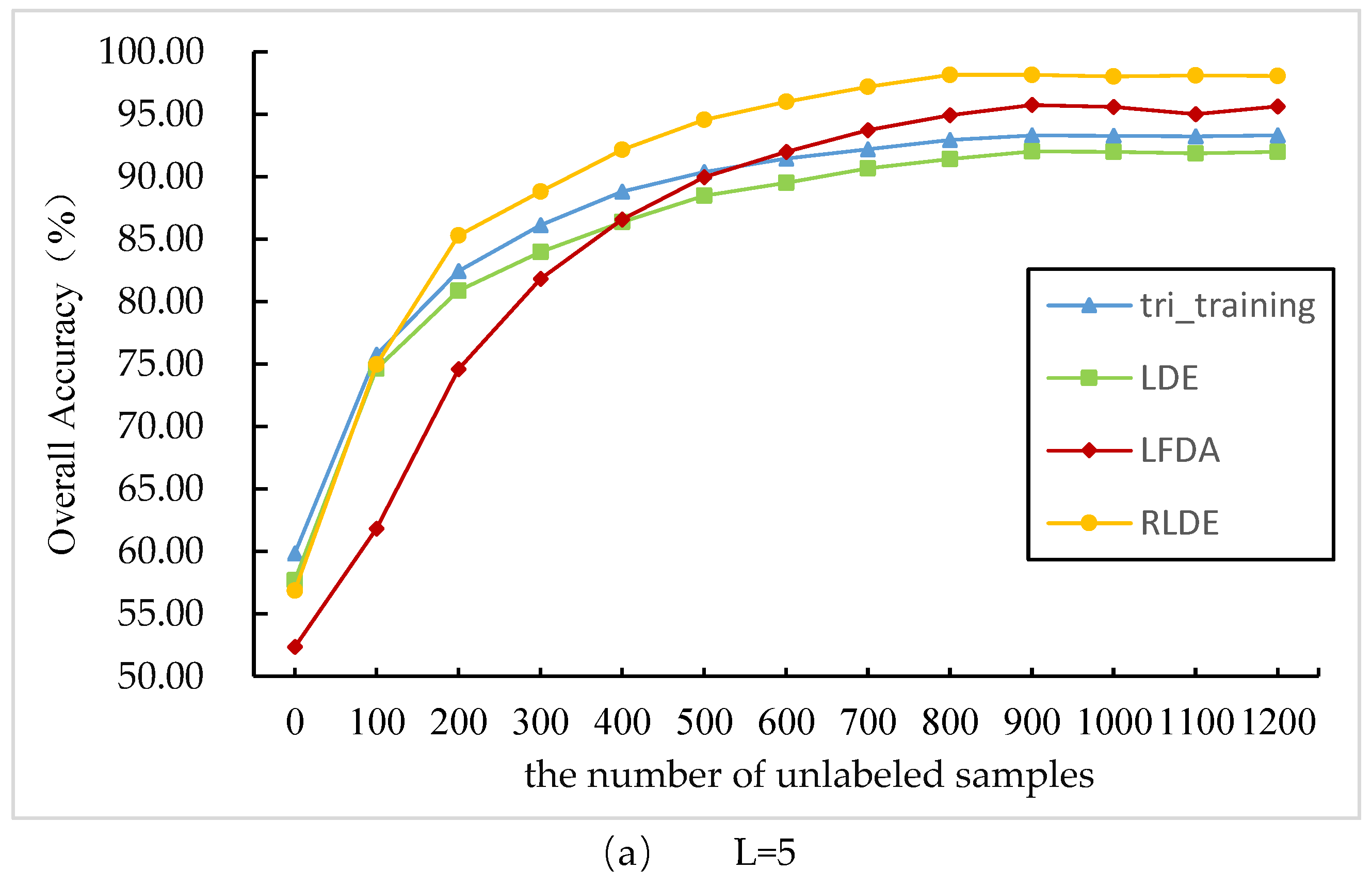
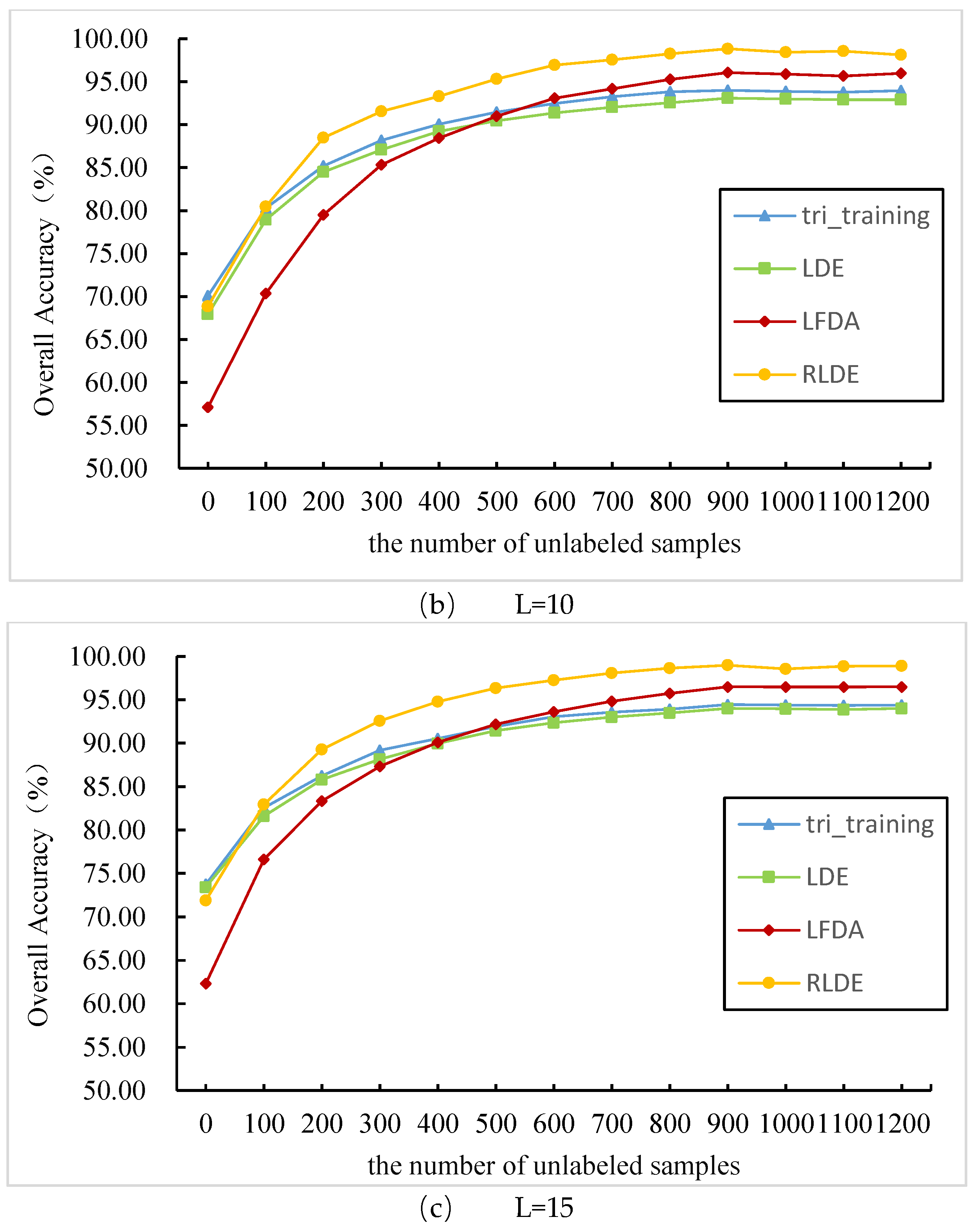
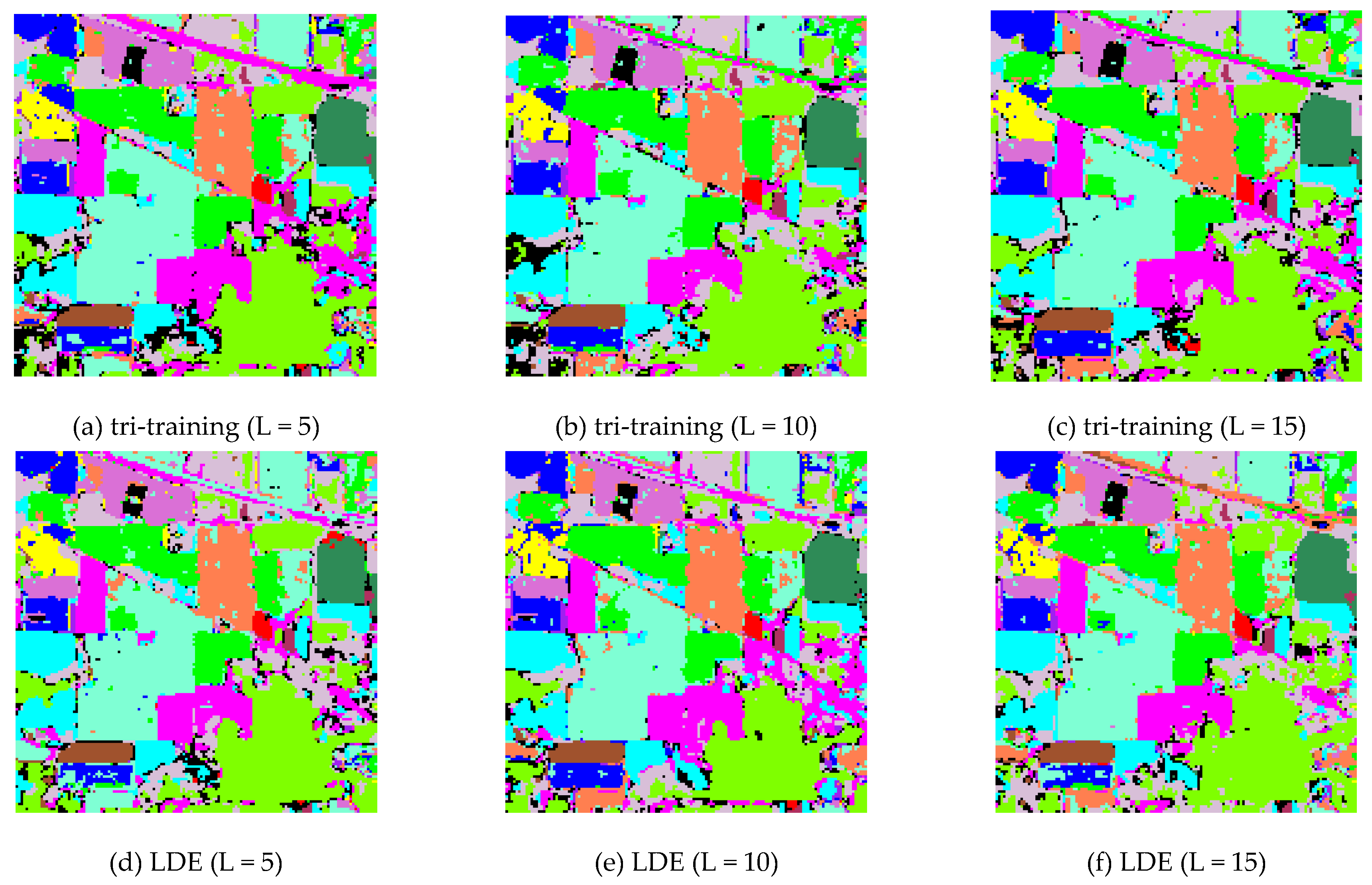
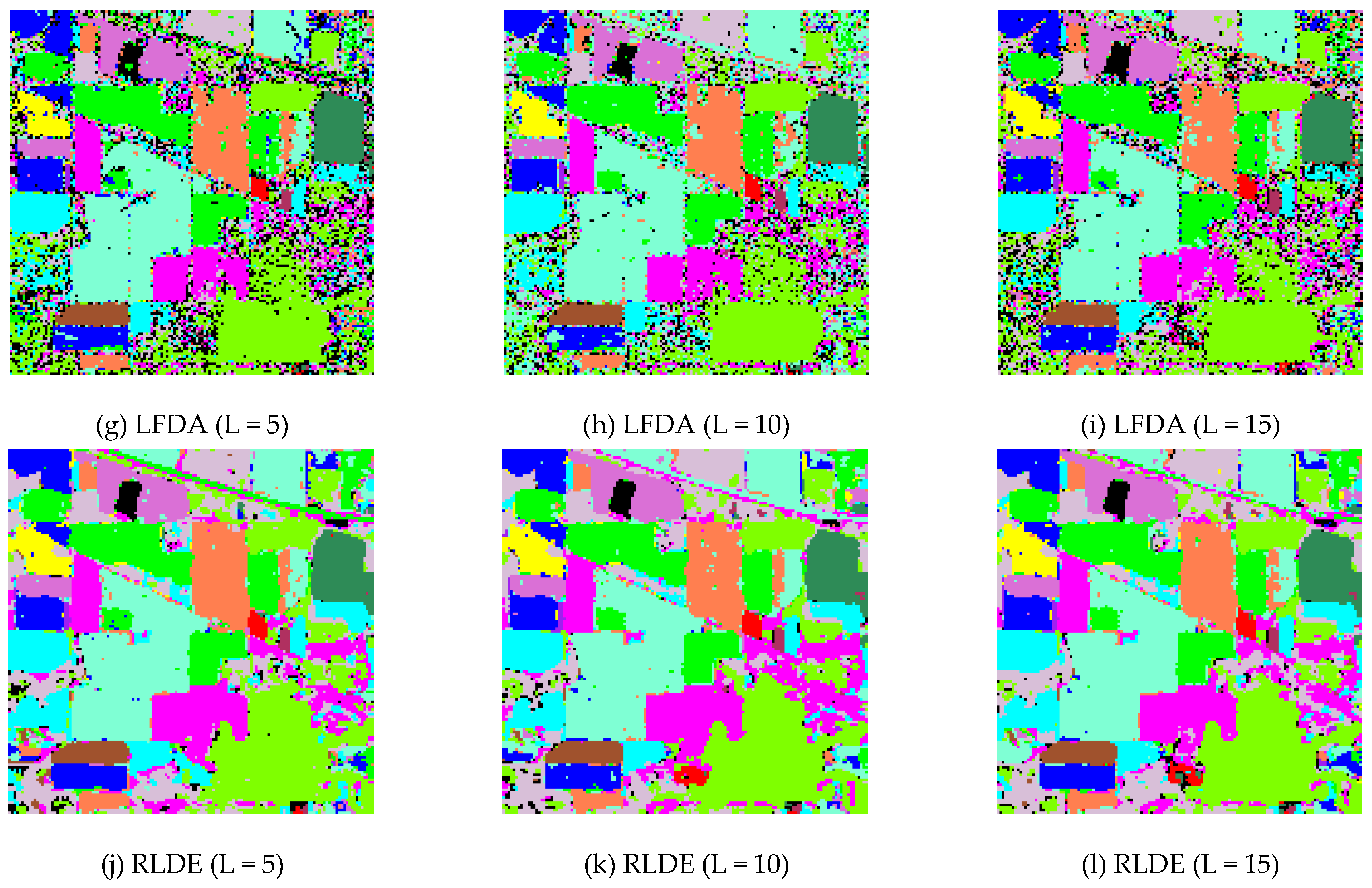
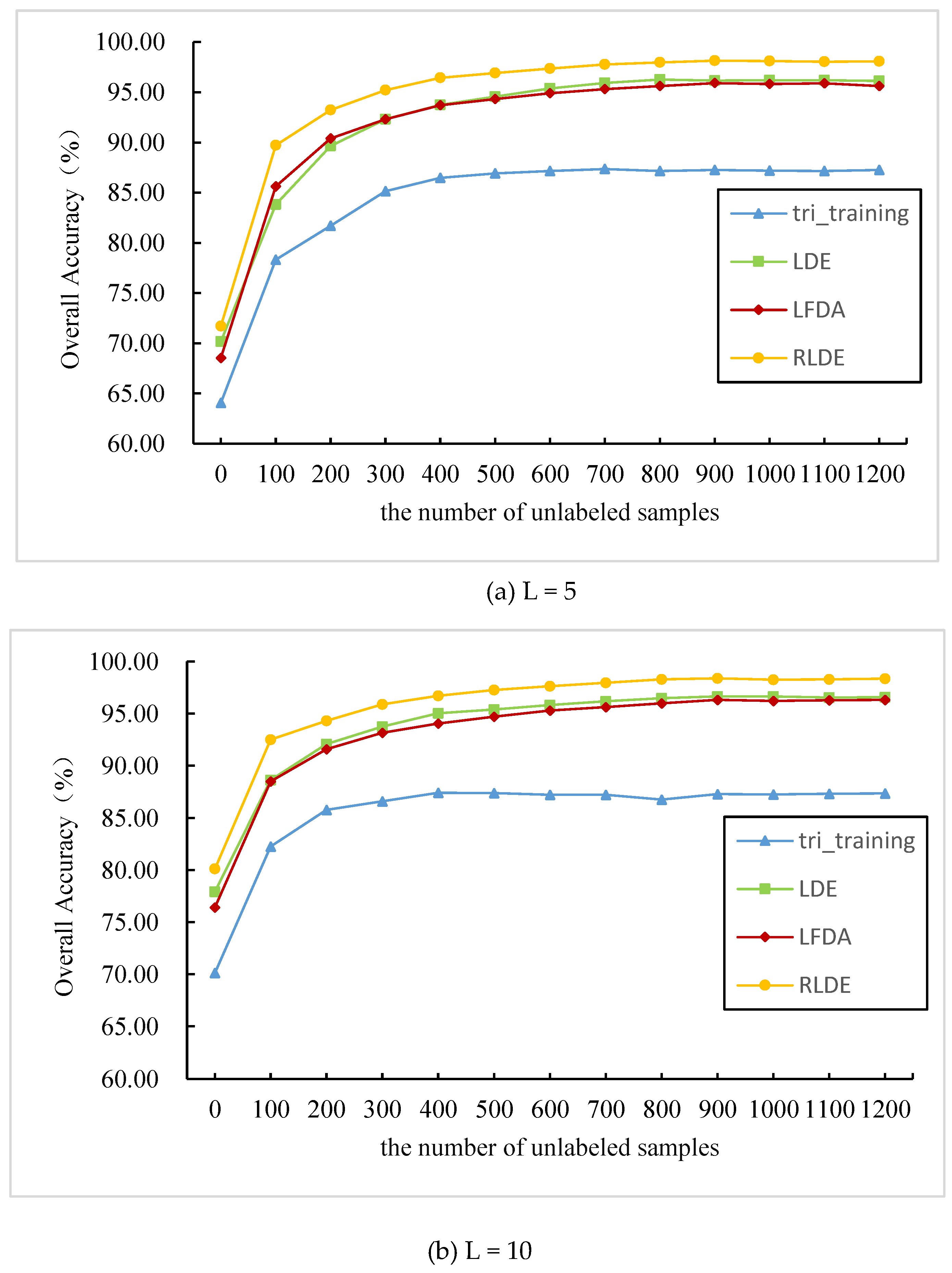
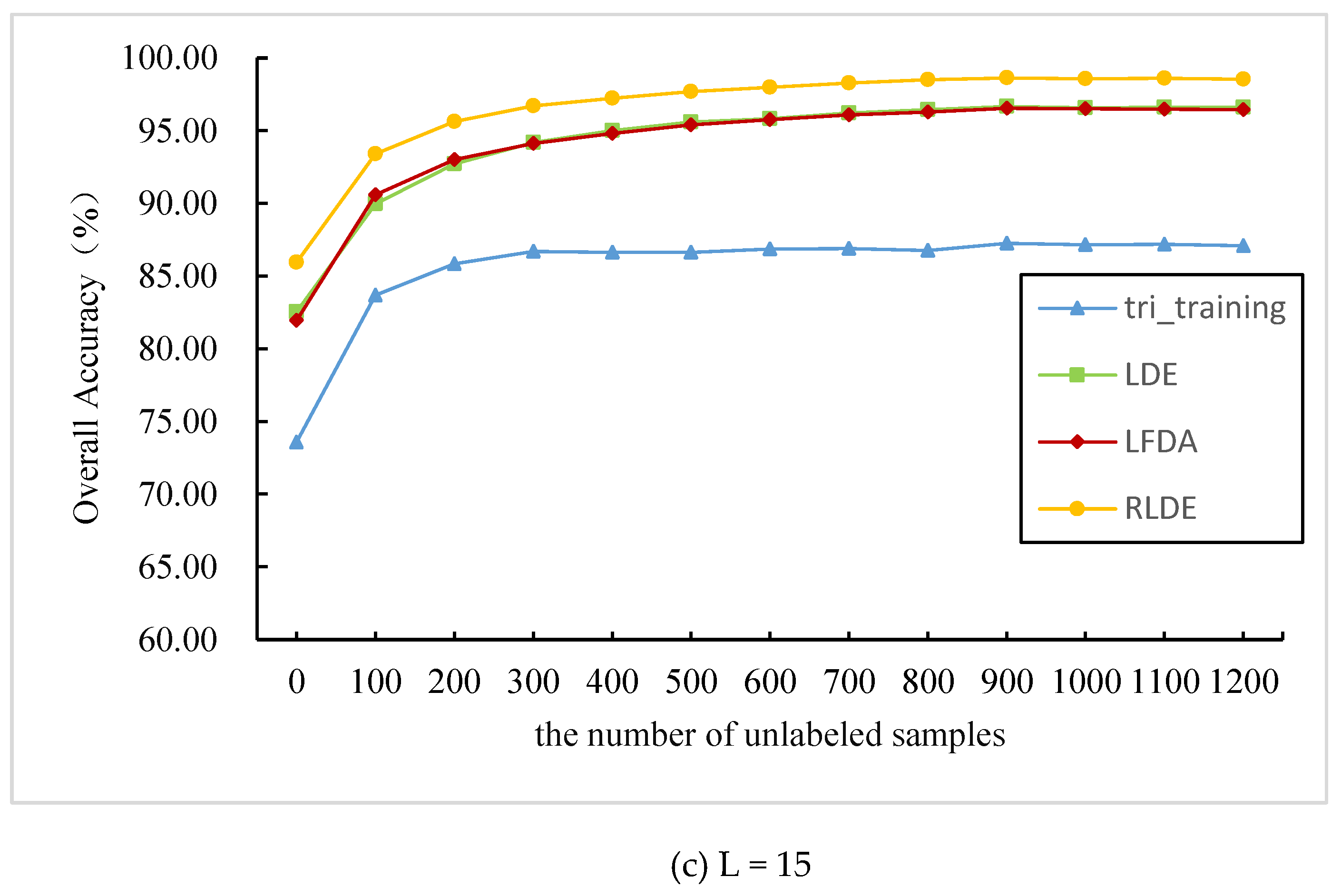
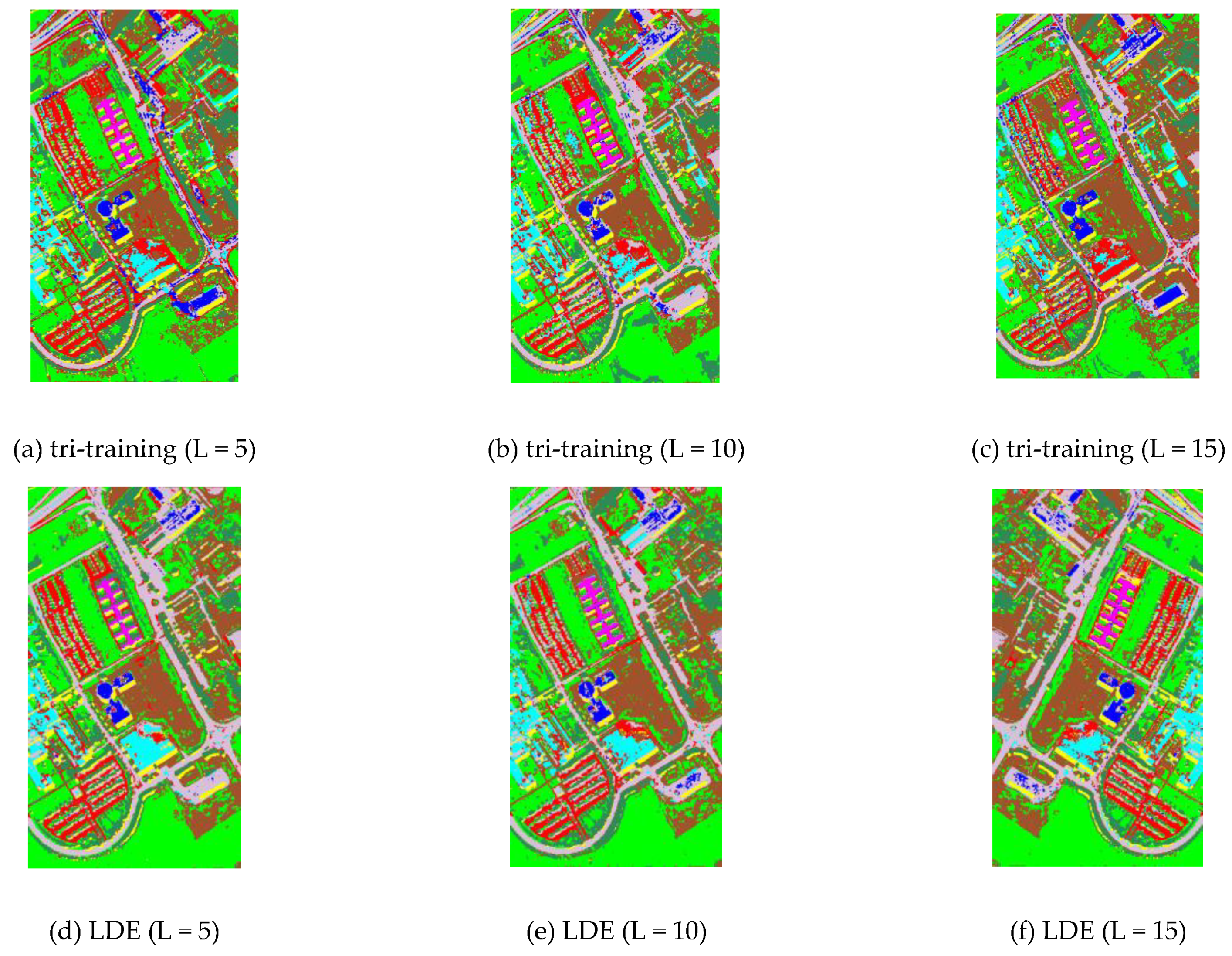
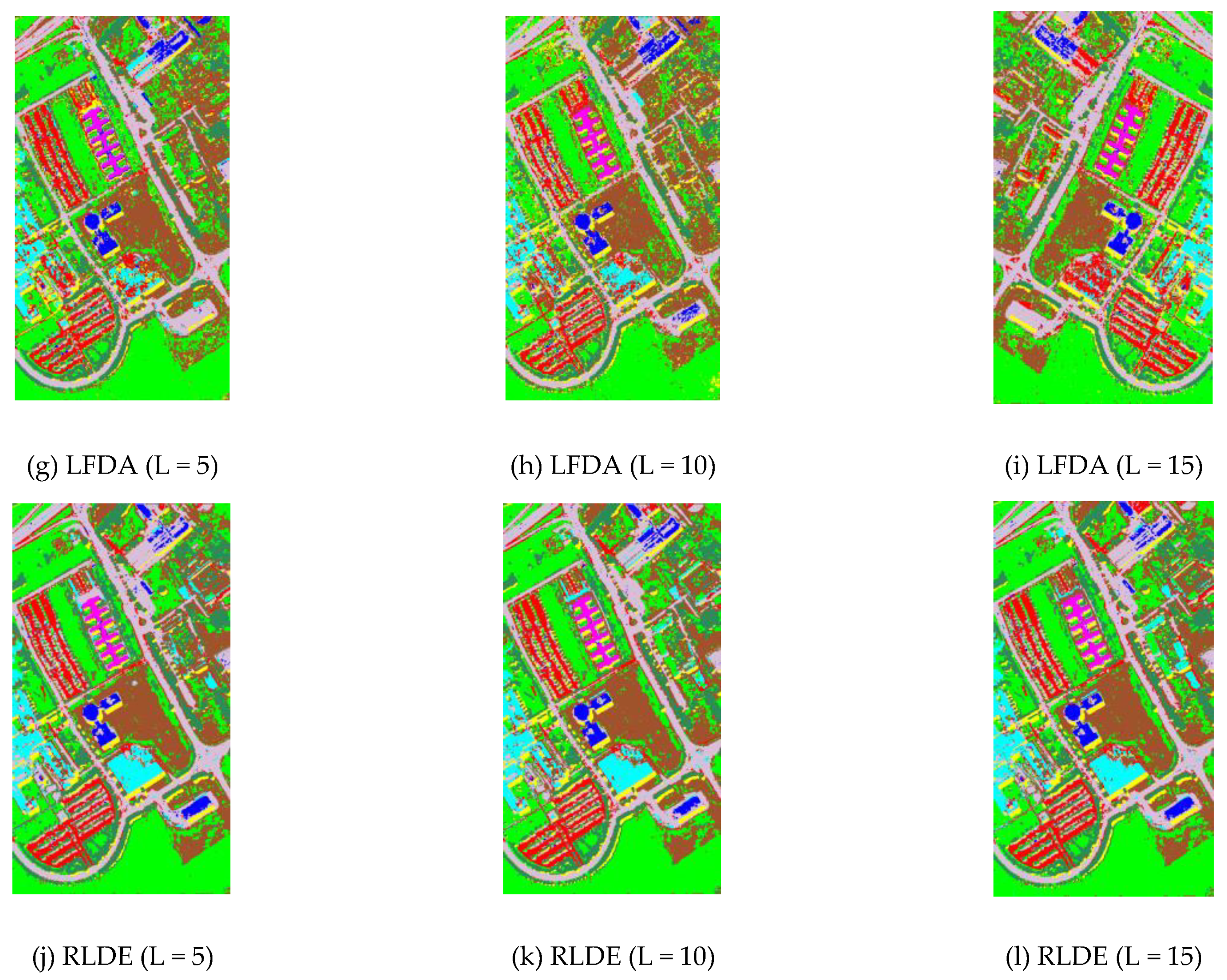
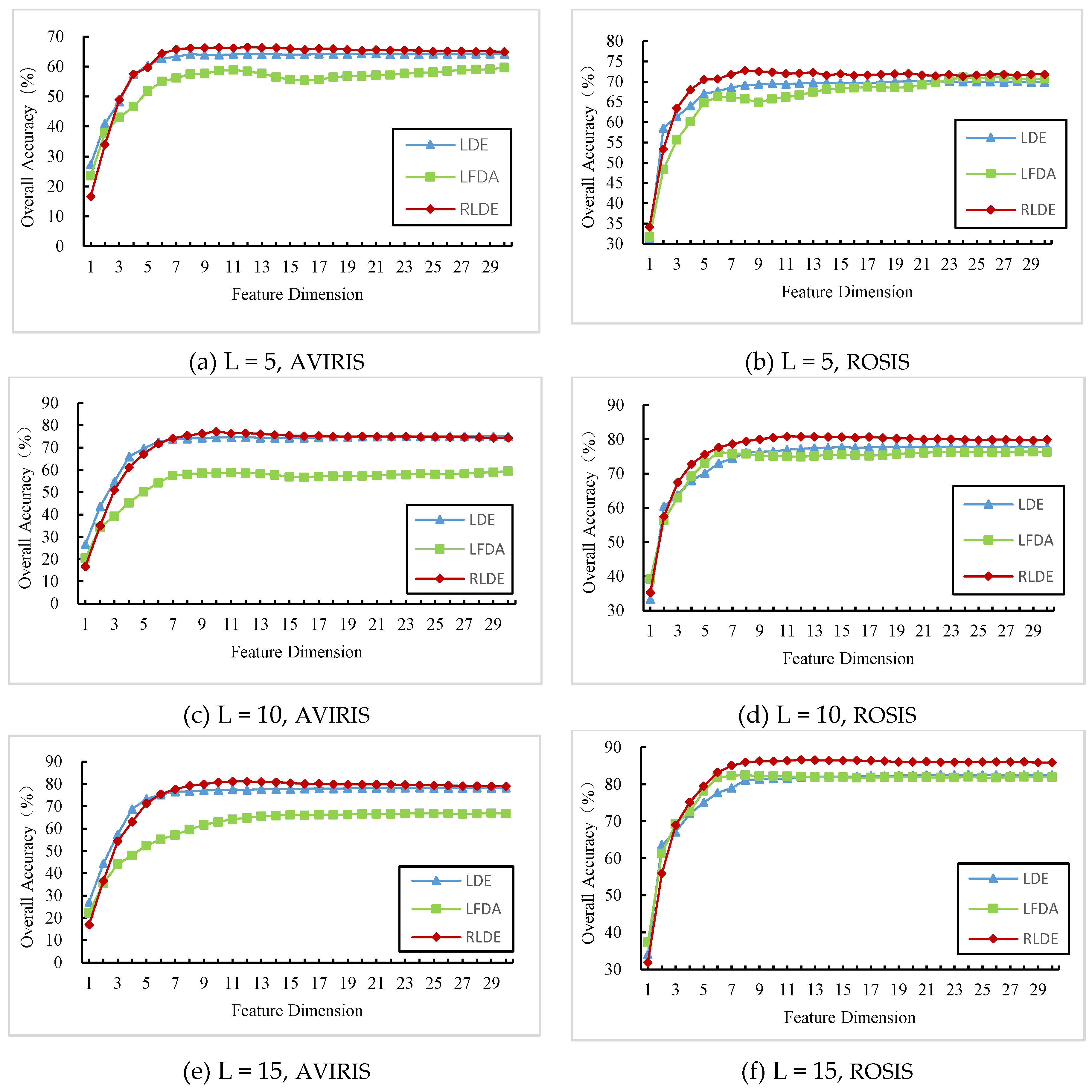
3.3. Comparison between the Different Feature Extraction Methods: AVIRIS Data

Figure 4 shows the classification results of the tri-training algorithm alone and the classification results of the tri-training algorithm based on the RLDE, LDE, and LFDA methods with the AVIRIS data. Specifically, the tri-training algorithm based on the LFDA method was proposed by Zhang and Jia in 2011 [48]. From Table 2 and Figure 4 and Figure 5, we can see that the classification accuracy is not significantly related to the number of initial samples when the number of unlabeled samples reaches 900 or more. For example, the classification accuracy using the LDE feature extraction method is 92.03%, 93.09%, and 94.01% when the number of initial samples is 5, 10, and 15, respectively. This indicates that the proposed algorithm is both reliable and robust. The proposed tri-training classification algorithm based on RLDE feature extraction performs the best among all the methods with different initial training samples. The OA is improved by 4.85%, 6.13%, and 2.42% compared with tri-training alone, LDE, and LFDA when the initial samples are 5. The OA is 4.84 %, 5.75%, and 2.78% higher than that of tri-training alone, LDE, and LFDA when the initial samples are 10. When the initial samples are 15, the classification accuracy is 4.53 %, 4.97%, and 2.48% higher than that of tri-training alone, LDE, and LFDA. Meanwhile, the classification accuracy based on the RLDE feature extraction method reaches 98.98%, which indicates that the proposed tri-training classification algorithm is superior to the other methods.

3.4. Comparison between the Different Feature Extraction Methods: ROSIS Data
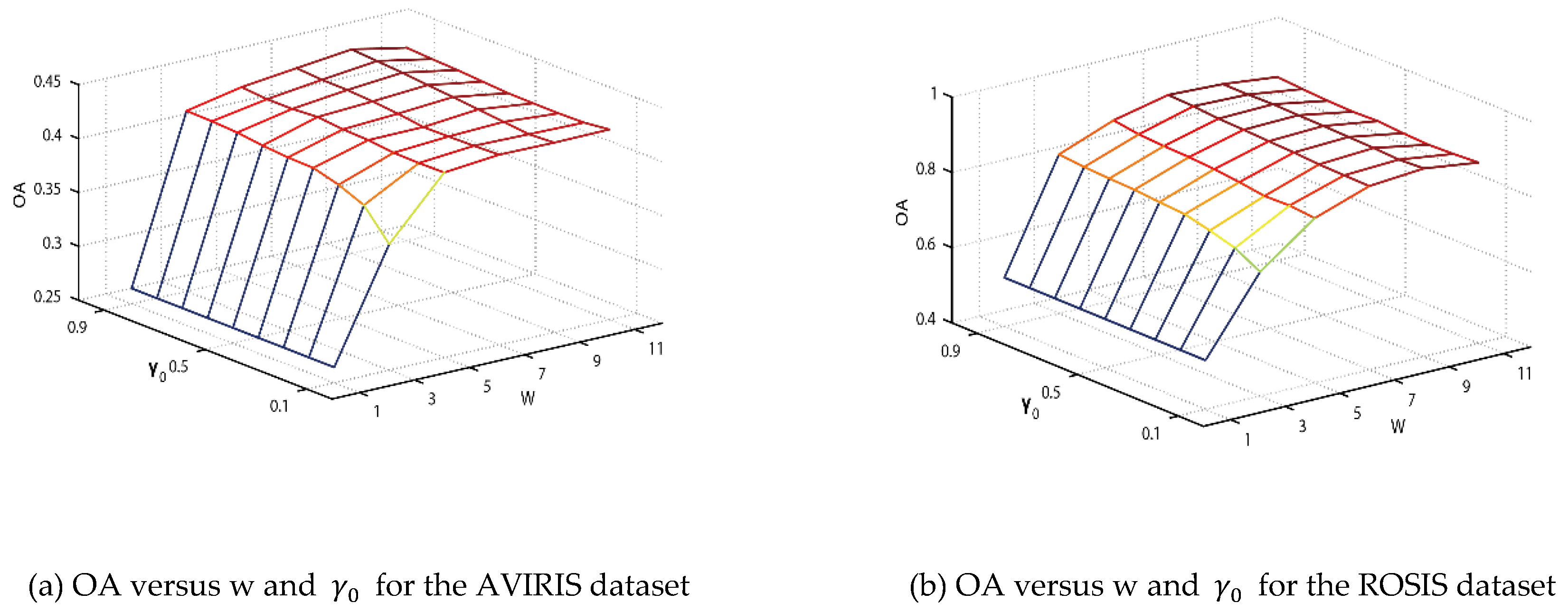
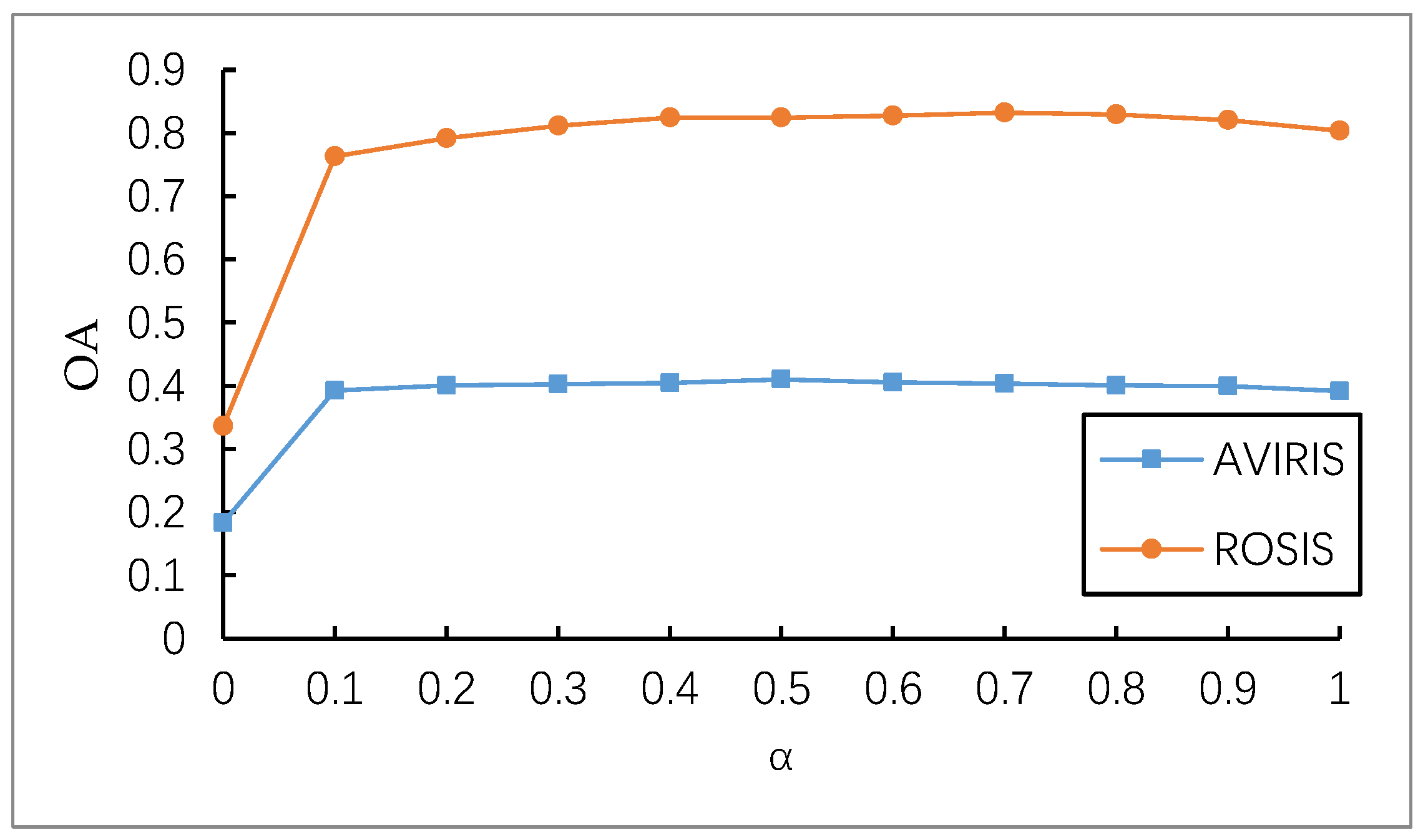
Figure 6 shows the classification results of the tri-training algorithm alone and the classification results of the tri-training algorithm based on the RLDE, LDE, and LFDA methods with the ROSIS data. From Table 3 and Figure 6 and Figure 7, we can see that, as the unlabeled samples are continuously added, the classification accuracy increases. However, when the unlabeled samples reach 700, the OA becomes stable. The classification accuracy is not significantly related to the number of initial samples when the number of unlabeled samples reaches 900 or more. For example, the classification accuracy using the LDE feature extraction method is 96.16%, 96.66%, and 96.66% when the number of initial samples is 5, 10, and 15, respectively. This indicates that the proposed algorithm is both reliable and robust. The proposed tri-training classification algorithm based on RLDE feature extraction performs the best among all the methods under the different initial training samples. The OA is improved by 10.79%, 1.73%, and 2.06% compared with tri-training alone, LDE, and LFDA when the initial samples are five. The OA is 10.97%, 1.73%, and 2.06% higher than that of tri-training alone, LDE, and LFDA when the initial samples are 10. When the initial samples are 15, the OA is 11.36%, 1.96%, and 2.08% higher than that of tri-training alone, LDE, and LFDA, respectively. Meanwhile, the classification accuracy based on the RLDE feature extraction method reaches 98.62%.

4. Discussion

In this section, the hyperparameters, w, γ 0 , and α are experimentally analyzed. In the SMF, both w and γ 0 affect the final precision. Hence, parameter w was chosen from the range of {1, 3, 5, 7, 9, 11}, and parameter γ 0 was chosen from the range of {0.1, 0.2, 0.3, …, 0.9}. In this parameter analysis, α was always set to 0.1. In the RLDE feature extraction method, α is the essential parameter, and was chosen from the range of {0, 0.1, 0.2, …, 1}. Parameter w was set to 3, and γ 0 was set to 0.2. Fifteen samples in each class were selected as the training set, and no addition operation was conducted with the training samples.
Figure 8 shows the OA versus w and γ 0 for the AVIRIS and ROSIS datasets, where it is shown that γ 0 has less impact on the classification accuracy than w. The optimal value of w is 9 for the AVIRIS dataset and 7 for the ROSIS dataset. The classification accuracy tends to be stable with parameter w within a range from 5 to 9. Figure 9 shows the OA versus α for the AVIRIS and ROSIS datasets. The optimal value of parameter α is 0.5 for the AVIRIS dataset and 0.7 for the ROSIS dataset.
The initial training sample conditions has an impact on the accuracy. In this section, optimal feature selection is discussed. In this analysis, the range of the spectral information dimension was set from 1 to 30. With 5, 10, and 15 initial training samples per class, and different feature extraction methods, we selected the optimal feature information for all the dimensions, as shown in Table 4 and Figure 10.
For the AVIRIS data, when the number of initial training samples per class is 5, the maximum OA and the dimension of LDE are 64.35% and 20, respectively. RLDE and LFDA can obtain the maximum OA when the feature information dimension is 12 and 30, respectively. When the number of initial training samples per class is 10, the maximum OA is obtained (75.16%) and the dimension of LDE is 26. RLDE and LFDA can obtain the maximum OA when the feature information dimension is 10 and 30, respectively. When the number of initial training samples per class is 15, the maximum OA is obtained (78.35%) and the dimension of PCA is 30. RLDE and LFDA can obtain the maximum OA when the feature information dimension is 10 and 24, respectively. Among the four different feature extraction methods, RLDE can obtain the highest classification accuracy and requires the smallest feature information dimension. With 5, 10, and 15 initial training samples per class, the feature information dimensions of all the methods were set as shown in Table 2 in the experiments.
For the ROSIS data, when the number of initial training samples per class is 5, the maximum OA and the dimension of LDE are 70.20% and 21, respectively. RLDE and LFDA can obtain the maximum OA when the feature information dimension is 8 and 24, respectively. When the number of initial training samples per class is 10, the maximum OA and the dimension of LDE are 77.93% and 24, respectively. RLDE and LFDA can obtain the maximum OA when the feature information dimension is 11 and 38, respectively. When the number of initial training samples per class is 15, the maximum OA and the dimension of LDE are 82.61% and 24, respectively. RLDE and LFDA can obtain the maximum OA when the feature information dimension is 12 and 8, respectively. Among the four different feature extraction methods, RLDE can obtain the highest classification accuracy and requires the smallest feature information dimension. With 5, 10, and 15 initial training samples per class, the feature information dimensions of all the methods were set based on Table 1 in the experiments.
Finally, we compared the proposed method with the other state-of-the-art deep learning methods of 1D-CNN, the CNN classifier proposed by Hu et al. [7], the five-layer CNN classifier proposed by Mei et al. [49], and the M3D-DCNN classifier proposed by He et al. [50]. All the methods, were compared under the same experimental settings (number of training samples, patch size, etc.) The OAs achieved by the different methods with the different HSI datasets are listed in Table 5. As can be seen, the proposed method shows a performance that is better than or comparable to the performance of the other four methods.

5. Conclusions

Hyperspectral sensors acquire hundreds of spectrally contiguous bands and provide abundant (but redundant) spectral information. In order to reduce the time consumption and improve the classification performance, it is necessary to extract the discriminant information before performing classification. In this paper, a novel semi-supervised tri-training algorithm for HSI classification has been proposed in conjunction with RLDE. The RLDE algorithm finds the optimal feature information, preserves the local information, and overcomes the singularity in the case of limited training samples. In the proposed algorithm, active learning is used to select the unlabeled samples, and ensemble learning is used to improve the classification result. In a comparison with other state-of-the-art deep learning methods, the proposed method achieved the highest classification accuracy with the least feature information.

Author Contributions

D.O. and K.T. conceived and designed the experiments; D.O. performed the experiments; D.O., K.T., J.Z., Y.C., and X.W. analyzed the data; D.O., K.T., Q.D., and J.Z. wrote the paper.

Funding

This research was supported in part by the National Natural Science Foundation of China (nos. 41871337, 41471356) and the Priority Academic Program Development of Jiangsu Higher Education Institutions.

Acknowledgments

The authors would like to thank Paolo Gamba at Pavia University for providing the ROSIS dataset and David Landgrede at Purdue University for providing the AVIRIS dataset.

Conflicts of Interest

The authors declare no conflict of interest.

References

  1. Ben-Dor, E.; Schläpfer, D.; Plaza, A.J.; Malthus, T. Hyperspectral remote sensing. In Airborne Measurements for Environmental Research: Methods and Instruments; Wiley-VCH Verlag & Co. KGaA: Weinheim, Germany, 2013; pp. 1249–1259. [Google Scholar]
  2. Groves, P.; Tian, L.F.; Bajwa, S.G.; Bajcsy, P. Hyperspectral image data mining for band selection in agricultural applications. Trans. ASAE 2004, 47, 895–907. [Google Scholar]
  3. Plaza, J.; Pérez, R.; Plaza, A.; Martínez, P.; Valencia, D. Mapping oil spills on sea water using spectral mixture analysis of hyperspectral image data. In Chemical and Biological Standoff Detection III; International Society for Optics and Photonics: Bellingham, WA, USA, 2005; Volume 5995, pp. 79–86. [Google Scholar]
  4. Iranzad, A. Hyperspectral Mineral Identification Using SVM and SOM; Brock University: St. Catharines, ON, Canada, 2013. [Google Scholar]
  5. Blum, A.; Mitchell, T. Combining labeled and unlabeled data with co-training. In Proceedings of the Eleventh Conference on Computational Learning Theory, Madisson, WI, USA, 24–26 July 1998; pp. 92–100. [Google Scholar]
  6. Peng, L.; Hui, Z.; Eom, K.B. Active deep learning for classification of hyperspectral images. IEEE J. Sel. Top. Appl. Earth Observat. Remote Sens. 2017, 10, 712–724. [Google Scholar]
  7. Hu, W.; Huang, Y.; Wei, L.; Zhang, F.; Li, H. Deep convolutional neural networks for hyperspectral image classification. J. Sens. 2015, 2015, 258619. [Google Scholar] [CrossRef]
  8. Song, J.; Zhang, H.; Li, X.; Gao, L.; Wang, M.; Hong, R. Self-supervised video hashing with hierarchical binary auto-encoder. IEEE Trans. Image Process. A Publ. IEEE Signal Process. Soc. 2018, 27, 3210. [Google Scholar] [CrossRef]
  9. Li, Y.; Zhang, H.; Shen, Q. Spectral-spatial classification of hyperspectral imagery with 3d convolutional neural network. Remote Sens. 2017, 9, 67. [Google Scholar] [CrossRef]
  10. Wang, X.; Gao, L.; Wang, P.; Sun, X.; Liu, X. Two-stream 3d convnet fusion for action recognition in videos with arbitrary size and length. IEEE Trans. Multimed. 2018, 20, 634–644. [Google Scholar] [CrossRef]
  11. Wang, X.; Gao, L.; Song, J.; Shen, H. Beyond frame-level cnn: Saliency-aware 3d cnn with lstm for video action recognition. IEEE Signal Process. Lett. 2017, 24, 510–514. [Google Scholar] [CrossRef]
  12. Mou, L.; Ghamisi, P.; Zhu, X.X. Deep recurrent neural networks for hyperspectral image classification. IEEE Trans. Geosci. Remote Sens. 2017, 55, 3639–3655. [Google Scholar] [CrossRef]
  13. Goldberg, A.B.; Zhu, X.; Singh, A.; Xu, Z.; Nowak, R. Multi-manifold semi-supervised learning. Ynh Lr on Arfal Nllgn & Mahn Larnng 2009, 5, 169–176. [Google Scholar]
  14. Tan, K.; Zhou, S.; Du, Q. Semisupervised discriminant analysis for hyperspectral imagery with block-sparse graph. IEEE Geosci. Remote Sens. Lett. 2015, 12, 1–5. [Google Scholar]
  15. Tuia, D.; Ratle, F.; Pacifici, F.; Kanevski, M.F. Active learning methods for remote sensing image classification. IEEE Trans. Geosci. Remote Sens. 2009, 47, 2218–2232. [Google Scholar] [CrossRef]
  16. Huang, R.; He, W. Using tri-training to exploit spectral and spatial information for hyperspectral data classification. In Proceedings of the International Conference on Computer Vision in Remote Sensing, Xiamen, China, 16–18 December 2012; pp. 30–33. [Google Scholar]
  17. Zhou, Z.H.; Li, M. Tri-training: Exploiting unlabeled data using three classifiers. IEEE Trans. Knowl. Data Eng. 2005, 17, 1529–1541. [Google Scholar] [CrossRef]
  18. Tan, K.; Li, E.; Du, Q.; Du, P. An efficient semi-supervised classification approach for hyperspectral imagery. Isprs J. Photogramm. Remote Sens. 2014, 97, 36–45. [Google Scholar] [CrossRef]
  19. Nixon, M. Feature Extraction & Image Processing for Computer Vision, 3rd ed.; Academic Press: Cambridge, MA, USA, 2008; pp. 595–599. [Google Scholar]
  20. Rui, Y.; Huang, T.S.; Chang, S.F. Image retrieval: Current techniques, promising directions, and open issues. J. Vis. Commun. Image Represent. 1999, 10, 39–62. [Google Scholar] [CrossRef]
  21. Hughes, G.F.; Hughes, G. On the mean accuracy of statistical pattern recognizers. IEEE Trans. Inf. Theory 1968, 14, 55–63. [Google Scholar] [CrossRef]
  22. Melgani, F.; Bruzzone, L. Classification of hyperspectral remote sensing images with support vector machines. IEEE Trans. Geosci. Remote Sens. 2004, 42, 1778–1790. [Google Scholar] [CrossRef] [Green Version]
  23. Pevný, T.; Filler, T.; Bas, P. Using High-Dimensional Image Models to Perform Highly Undetectable Steganography; Springer: Berlin/Heidelberg, Germany, 2010; pp. 161–177. [Google Scholar]
  24. Yu, L.; Liu, H. Feature selection for high-dimensional data: A fast correlation-based filter solution. In Proceedings of the Twentieth International Conference on Machine Learning, Washington, DC, USA, 21–24 August 2003; pp. 856–863. [Google Scholar]
  25. Draper, B.A.; Baek, K.; Bartlett, M.S.; Beveridge, J.R. Recognizing faces with pca and ica. Comput. Vis. Image Underst. 2003, 91, 115–137. [Google Scholar] [CrossRef]
  26. Liu, Z.P. Linear Discriminant Analysis; John Wiley & Sons, Inc.: Hoboken, NJ, USA, 2006; pp. 2464–2485. [Google Scholar]
  27. Kukharev, G.; Forczmaski, P.L. Face recognition by means of two-dimensional direct linear discriminant analysis. In Proceedings of the 8th International Conference on Pattern Recognition and Information Processing, Minsk, Belarus, 18–20 May 2005; Volume 280. [Google Scholar]
  28. Li, H.; Jiang, T.; Zhang, K. Efficient and robust feature extraction by maximum margin criterion. IEEE Trans. Neural Netw. 2006, 17, 157–165. [Google Scholar] [CrossRef]
  29. Bilgin, G.; Erturk, S.; Yildirim, T. Nonlinear dimension reduction methods and segmentation of hyperspectral images. In Proceedings of the IEEE Signal Processing, Communication and Applications Conference, Aydin, Turkey, 20–22 April 2008; pp. 1–4. [Google Scholar]
  30. Camps-Valls, G.; Gomez-Chova, L.; Munoz-Mari, J.; Rojo-Alvarez, J.L. Kernel-based framework for multitemporal and multisource remote sensing data classification and change detection. IEEE Trans. Geosci. Remote Sens. 2008, 46, 1822–1835. [Google Scholar] [CrossRef]
  31. Song, J.; Gao, L.; Nie, F.; Shen, H.; Yan, Y.; Sebe, N. Optimized graph learning with partial tags and multiple features for image and video annotation. IEEE Trans. Image Process. 2016, 25, 4999–5011. [Google Scholar] [CrossRef]
  32. Zhang, Z.; Wang, J.; Zha, H. Adaptive manifold learning. IEEE Trans. Pattern Anal. Mach. Intell. 2012, 34, 253–265. [Google Scholar] [CrossRef]
  33. Wu, W.; Massart, D.L.; Jong, S.D. The kernel pca algorithms for wide data. Part i: Theory and algorithms. Chemom. Intell. Lab. Syst. 1997, 36, 165–172. [Google Scholar] [CrossRef]
  34. Mika, S.; Rätsch, G.; Weston, J.; Schölkopf, B.; Müller, K.R. Fisher discriminant analysis with kernels. In Neural Networks for Signal Processing IX: Proceedings of the 1999 IEEE Signal Processing Society Workshop; The Institute of Electrical and Electronics Engineers, Inc.: New York, NY, USA, 1999; pp. 41–48. [Google Scholar]
  35. Song, J.; Yang, Y.; Li, X.; Huang, Z.; Yang, Y. Robust hashing with local models for approximate similarity search. IEEE Trans. Cybern. 2014, 44, 1225. [Google Scholar] [CrossRef]
  36. Song, J.; Yang, Y.; Huang, Z.; Shen, H.T.; Luo, J. Effective multiple feature hashing for large-scale near-duplicate video retrieval. IEEE Trans. Multimed. 2013, 15, 1997–2008. [Google Scholar] [CrossRef]
  37. Tenenbaum, J.B.; De, S.V.; Langford, J.C. A global geometric framework for nonlinear dimensionality reduction. Science 2000, 290, 2319. [Google Scholar] [CrossRef]
  38. Roweis, S.T.; Saul, L.K. Nonlinear dimensionality reduction by locally linear embedding. Science 2000, 290, 2323. [Google Scholar] [CrossRef]
  39. He, X.; Cai, D.; Yan, S.; Zhang, H.J. Neighborhood preserving embedding. In Proceedings of the Tenth IEEE International Conference on Computer Vision, Beijing, China, 17–21 October 2005; pp. 1208–1213. [Google Scholar]
  40. Chen, H.T.; Chang, H.W.; Liu, T.L. Local discriminant embedding and its variants. In Proceedings of the IEEE Computer Society Conference on Computer Vision & Pattern Recognition, San Diego, CA, USA, 20–25 June 2005; pp. 846–853. [Google Scholar]
  41. Zhou, Y.; Peng, J.; Chen, C.L.P. Dimension reduction using spatial and spectral regularized local discriminant embedding for hyperspectral image classification. IEEE Trans. Geosci. Remote Sens. 2015, 53, 1082–1095. [Google Scholar] [CrossRef]
  42. Liao, W.; Pizurica, A.; Philips, W.; Pi, Y. Feature extraction for hyperspectral images based on semi-supervised local discriminant analysis. IEEE Trans. Geosci. Remote Sens. 2013, 51, 401–404. [Google Scholar]
  43. Sugiyama, M.; Idé, T.; Nakajima, S.; Sese, J. Semi-Supervised Local Fisher Discriminant Analysis for Dimensionality Reduction; Springer: Berlin/Heidelberg, Germany, 2008; pp. 35–61. [Google Scholar]
  44. Hua, G.; Brown, M.; Winder, S. Discriminant embedding for local image descriptors. In Proceedings of the IEEE International Conference on Computer Vision, Rio De Janeiro, Brazil, 14–21 October 2007; pp. 1–8. [Google Scholar]
  45. Wan, M.; Yang, G.; Lai, Z.; Jin, Z. Feature extraction based on fuzzy local discriminant embedding with applications to face recognition. IET Comput. Vis. 2011, 5, 301–308. [Google Scholar] [CrossRef]
  46. Pang, Y.; Yu, N. Regularized local discrimimant embedding. In Proceedings of the IEEE International Conference on Acoustics, Speech and Signal Processing, Toulouse, France, 14–19 May 2006; p. III. [Google Scholar]
  47. Tan, K.; Zhu, J.; Du, Q.; Wu, L.; Du, P. A novel tri-training technique for semi-supervised classification of hyperspectral images based on diversity measurement. Remote Sens. 2016, 8, 749. [Google Scholar] [CrossRef]
  48. Zhang, G.; Jia, X. Feature selection using kernel based local fisher discriminant analysis for hyperspectral image classification. In Proceedings of the IEEE International Geoscience and Remote Sensing Symposium, Vancouver, BC, Canada, 24–29 July 2011; pp. 1728–1731. [Google Scholar]
  49. Mei, S.; Ji, J.; Bi, Q.; Hou, J.; Qian, D.; Wei, L. Integrating spectral and spatial information into deep convolutional neural networks for hyperspectral classification. In Proceedings of the IEEE International Geoscience and Remote Sensing Symposium, Beijing, China, 10–15 July 2016. [Google Scholar]
  50. He, M.; Bo, L.; Chen, H. Multi-scale 3d deep convolutional neural network for hyperspectral image classification. In Proceedings of the IEEE International Conference on Image Processing, Beijing, China, 17–20 September 2017. [Google Scholar]
Figure 1. (a) Pseudocolor composite of the Airborne Visible/Infrared Imaging Spectrometer (AVIRIS) Indian Pines dataset. (b) The test area with 16 mutually exclusive ground-truth classes.
Remotesensing 11 00654 g001
Figure 2. (a) Pseudocolor composite of the Reflective Optics System Imaging Spectrometer (ROSIS) Pavia scene. (b) The test area with nine mutually exclusive ground-truth classes.
Remotesensing 11 00654 g002
Figure 3. The results of cooperative training classification based on RLDE local feature extraction.
Remotesensing 11 00654 g003
Figure 4. AVIRIS data classification accuracy, as obtained by the different feature extraction methods under different initial training samples.
Remotesensing 11 00654 g004aRemotesensing 11 00654 g004b
Figure 5. Co-training classification results based on the different feature extraction methods.
Remotesensing 11 00654 g005aRemotesensing 11 00654 g005b
Figure 6. AVIRIS data classification accuracy, as obtained by the different feature extraction methods under different initial training samples.
Remotesensing 11 00654 g006aRemotesensing 11 00654 g006b
Figure 7. Co-training classification results based on the different feature extraction methods.
Remotesensing 11 00654 g007aRemotesensing 11 00654 g007b
Figure 8. Overall accuracy (OA) versus w and γ 0 for the AVIRIS and ROSIS datasets.
Remotesensing 11 00654 g008
Figure 9. OA versus α for the AVIRIS and ROSIS datasets.
Remotesensing 11 00654 g009
Figure 10. AVIRIS data and ROSIS data classification accuracy for different feature dimension, as obtained by the different feature extraction methods under different initial training samples.
Remotesensing 11 00654 g010
Table 1. Results of cooperative training classification based on the regularized local discriminant embedding (RLDE) local feature extraction method (%).
12345678910
AVIRISNon- SMF543.1161.5969.3173.8877.5879.9381.9183.2984.8686.15
1053.0166.7172.7077.0479.5681.8683.6984.6485.9586.96
1560.5769.5274.9278.2180.9182.5683.9485.4486.4587.35
SMF559.0179.0186.6090.7593.3694.9896.3797.1397.8398.34
1069.7783.5188.9392.1494.4895.6796.5597.3597.9298.35
1576.5486.0090.9693.4795.2396.2197.1497.7998.3098.65
ROSISNon- SMF562.4579.9884.8386.5387.5188.4389.1089.7890.1990.58
1069.8383.3586.6888.7289.6190.3690.8791.2791.6391.94
1575.3684.3587.6588.8889.8690.5490.8891.3891.7092.05
SMF571.7089.7193.2495.2196.4396.9297.3697.7597.9698.14
1080.1192.5294.3395.9196.7397.2797.6397.9698.2998.39
1585.9493.4195.6396.6997.2397.6897.9798.2698.4998.62
Table 2. Tri-training classification results based on the different feature extraction methods (%).
12345678910
L = 5Tri-trainingOA59.8375.7682.4686.1388.8090.3891.4492.2192.9393.31
Kappa55.4172.3879.9684.1587.2189.0190.2391.1191.9392.36
LDEOA57.6974.6580.8883.9986.3688.4789.5190.6791.4292.03
Kappa56.6571.9378.5081.9384.5786.9788.1289.4490.3090.99
LFDAOA52.3461.8374.6181.8486.5689.9592.0193.7494.9295.74
Kappa61.0970.8079.2084.2588.2390.9792.5694.0895.0295.67
RLDEOA56.8674.9685.2988.8292.1494.5695.9997.1998.1698.16
Kappa52.7871.8783.3787.3491.0793.8195.4496.8097.9097.90
L = 10Tri-trainingOA70.0780.2985.2188.1790.0791.4792.4993.2593.8194.00
Kappa66.5677.5183.1086.5188.6890.2791.4392.3192.9493.16
LDEOA67.9378.9584.4887.0689.2290.4691.3792.0492.5493.09
Kappa67.3277.1582.8085.4887.8989.2890.3091.0191.5892.18
LFDAOA57.0970.3679.5185.3188.4291.0093.0794.1695.2896.06
Kappa69.0775.2182.2187.0689.5091.7093.5394.3295.2596.00
RLDEOA68.8580.4588.4891.5393.3295.3296.9697.5498.2698.84
Kappa65.5978.1186.9590.4192.4294.6796.5397.2098.0298.68
L = 15Tri-trainingOA73.7582.5686.2589.1790.5591.9393.0493.5793.9294.45
Kappa70.6080.1284.3187.6489.2290.8092.0792.6793.0793.68
LDEOA73.4381.6185.8388.1589.9791.4392.3693.0393.4894.01
Kappa72.6879.8284.2186.7088.6690.2991.3292.0792.5993.21
LFDAOA62.3276.6283.3687.3190.1192.1793.6294.8595.7496.50
Kappa68.9180.6885.3688.3190.6292.3993.6294.8095.6096.36
RLDEOA71.8982.9689.2992.5794.7796.3497.2898.0898.6398.98
Kappa68.9280.8287.8891.5794.0595.8396.9097.8298.4498.84
Table 3. Tri-training classification results based on the different feature extraction methods (%).
12345678910
L = 5tri-trainingOA64.0578.3081.7185.1386.4786.9187.1687.3587.1487.26
Kappa55.6271.6776.0580.2582.0782.7583.0983.3583.1183.26
LDEOA70.1583.8089.6392.2993.7294.5695.3795.9296.2696.16
Kappa62.7878.4286.1489.6791.6192.7593.8294.5695.0294.89
LFDAOA68.5485.6190.4092.3093.7094.3394.8895.3195.6095.90
Kappa65.1681.6287.1489.5391.4092.2292.9993.5793.9794.36
RLDEOA71.7089.7193.2495.2196.4396.9297.3697.7597.9698.14
Kappa67.1687.2291.2493.6895.2295.8496.4196.9397.2197.44
L = 10tri-trainingOA70.1282.2785.7886.5987.4287.3987.2387.2286.7587.30
Kappa63.0376.5380.9882.2183.3483.3983.2583.2482.7083.37
LDEOA77.9288.6492.1093.7695.0395.4095.8496.1996.5096.66
Kappa72.2784.8189.3891.6493.3793.8694.4594.9295.3495.55
LFDAOA76.4188.5291.5993.1894.0794.7395.3295.6595.9896.33
Kappa73.8586.0989.4191.2492.2493.0293.7694.1794.5795.04
RLDEOA80.1192.5294.3395.9196.7397.2797.6397.9698.2998.39
Kappa76.4590.3892.5394.5195.5896.3096.7897.2197.6697.80
L = 15tri-trainingOA73.5883.7085.8586.7086.6486.6286.8486.8986.7587.26
Kappa66.9478.4181.2482.4682.4482.4882.8182.8882.7483.37
LDEOA82.5489.9892.7194.2095.0295.5895.8196.2196.4596.66
Kappa77.7286.6690.2492.2493.3594.1094.4194.9595.2895.55
LFDAOA81.9490.5992.9994.1294.8295.3895.7596.0996.3096.54
Kappa79.6187.8490.5692.0192.9793.7094.2094.6494.9295.26
RLDEOA85.9493.4195.6396.6997.2397.6897.9798.2698.4998.62
Kappa83.6191.4594.2195.5696.2596.8597.2297.6297.9498.10
Table 4. The optimal feature number and classification accuracy of the different feature extraction methods under different initial training sample conditions.
Training SamplesL = 5L = 10L = 15
Feature Extraction Method
AVIRISLDE64.35%(20)75.16%(26)78.35%(30)
LFDA59.72%(30)59.48%(30)66.90%(24)
RLDE66.54%(12)77.23%(10)81.20%(11)
ROSISLDE70.20%(21)77.93%(24)82.61%(24)
RLDE72.76%(8)80.95%(11)86.62%(12)
LFDA71.09%(24)76.43%(28)82.50%(8)
Table 5. The classification OA of the different deep learning methods with the different hyperspectral image (HSI) datasets.
Dataset1D-CNNHu et al. [7] Mei et al. [49]M3D-DCNN [50]Proposed Method
Indian Pines82.39%90.07%95.70%97.61%98.98%
Pavia Univ.93.29%92.74%98.00%98.49%98.62%

