Efficient Identification of Corn Cultivation Area with Multitemporal Synthetic Aperture Radar and Optical Images in the Google Earth Engine Cloud Platform


Abstract
:
1. Introduction
2. Materials
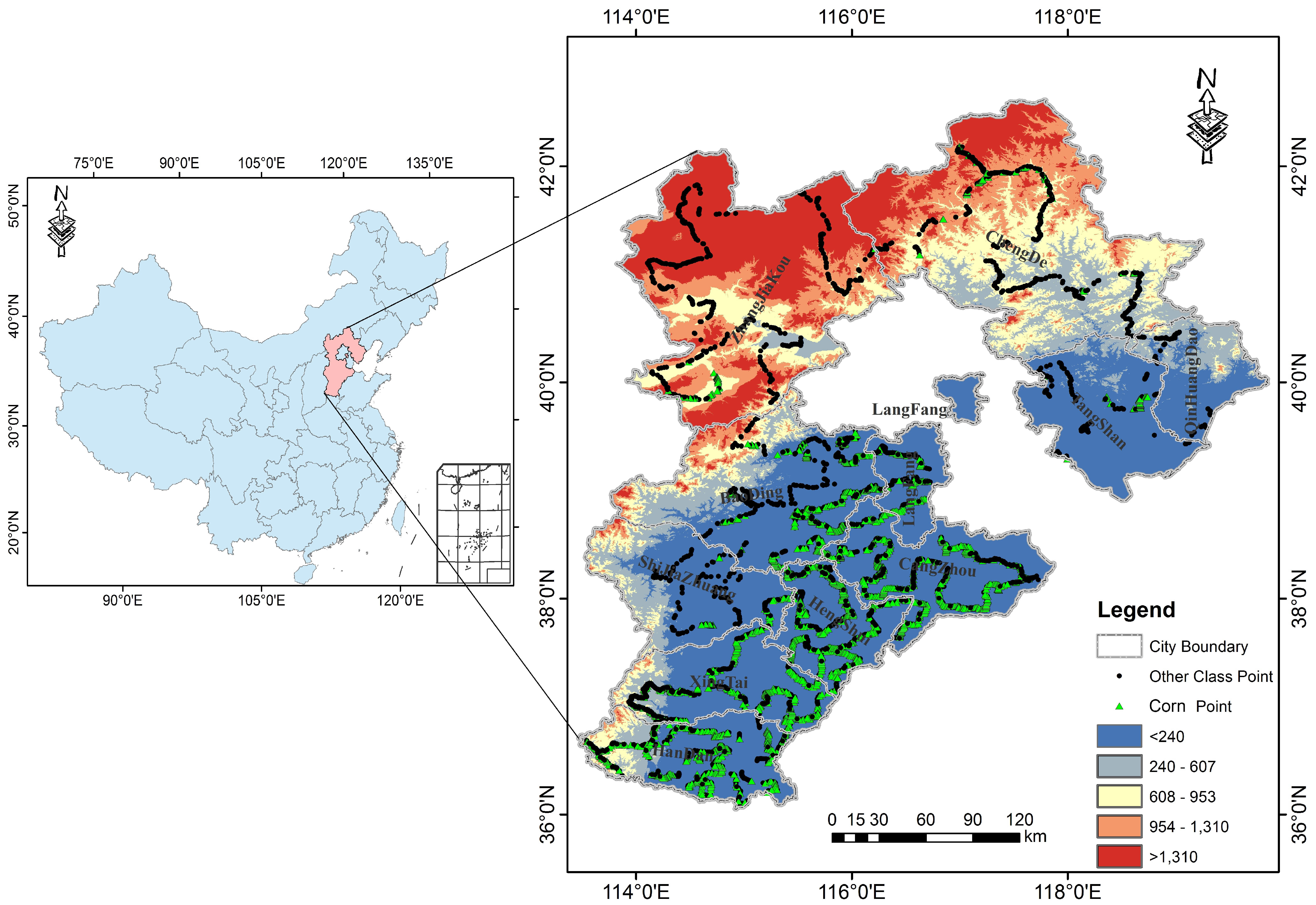
2.1. Study Area
2.2. Sentinel-2 Imagery and Preprocessing
2.3. Sentinel-1 SAR Data
2.4. Reference Dataset
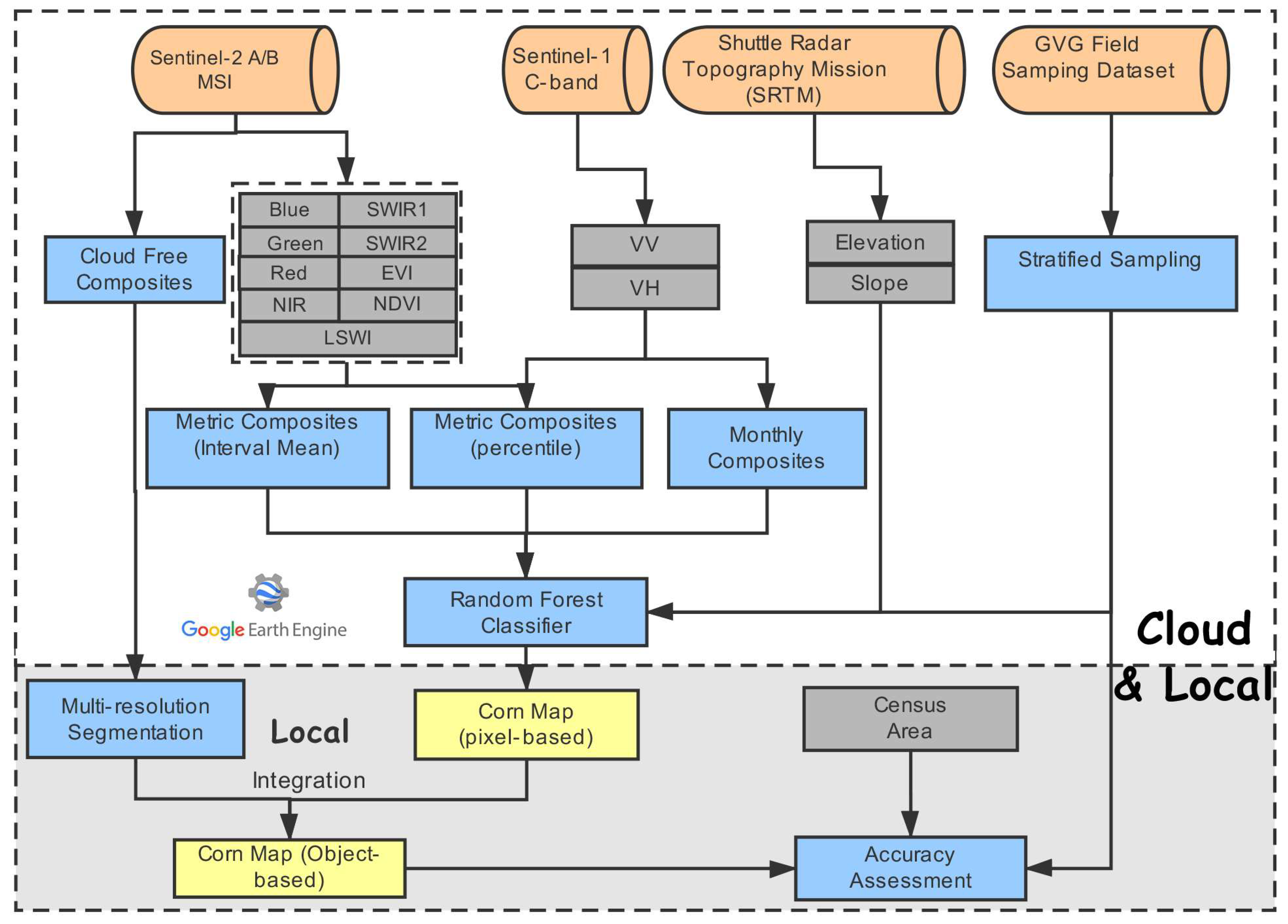
3. Methodology
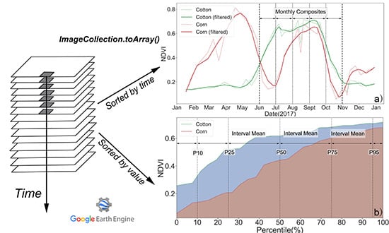
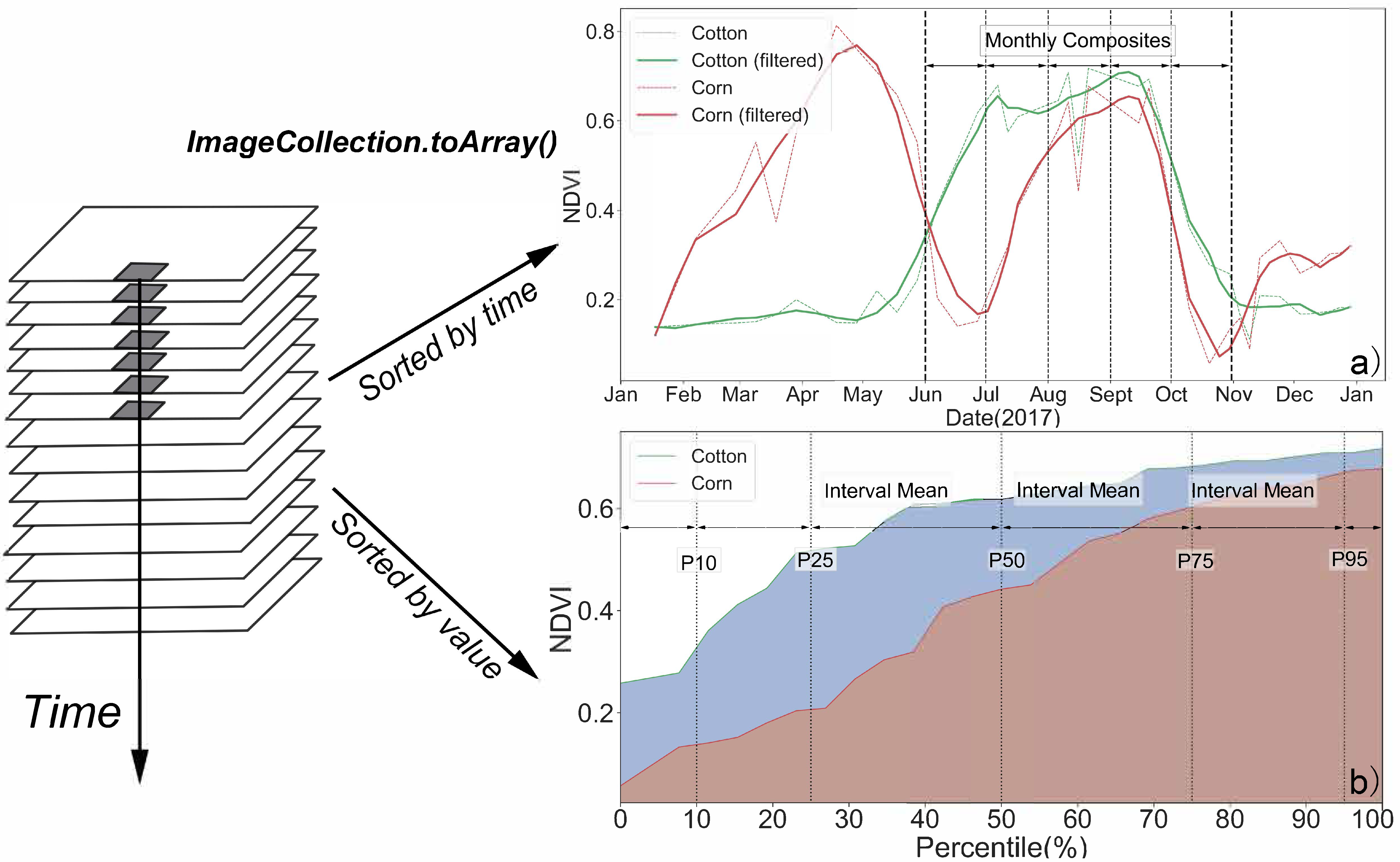
3.1. Image Compositing
3.2. Pixel-Based Classification
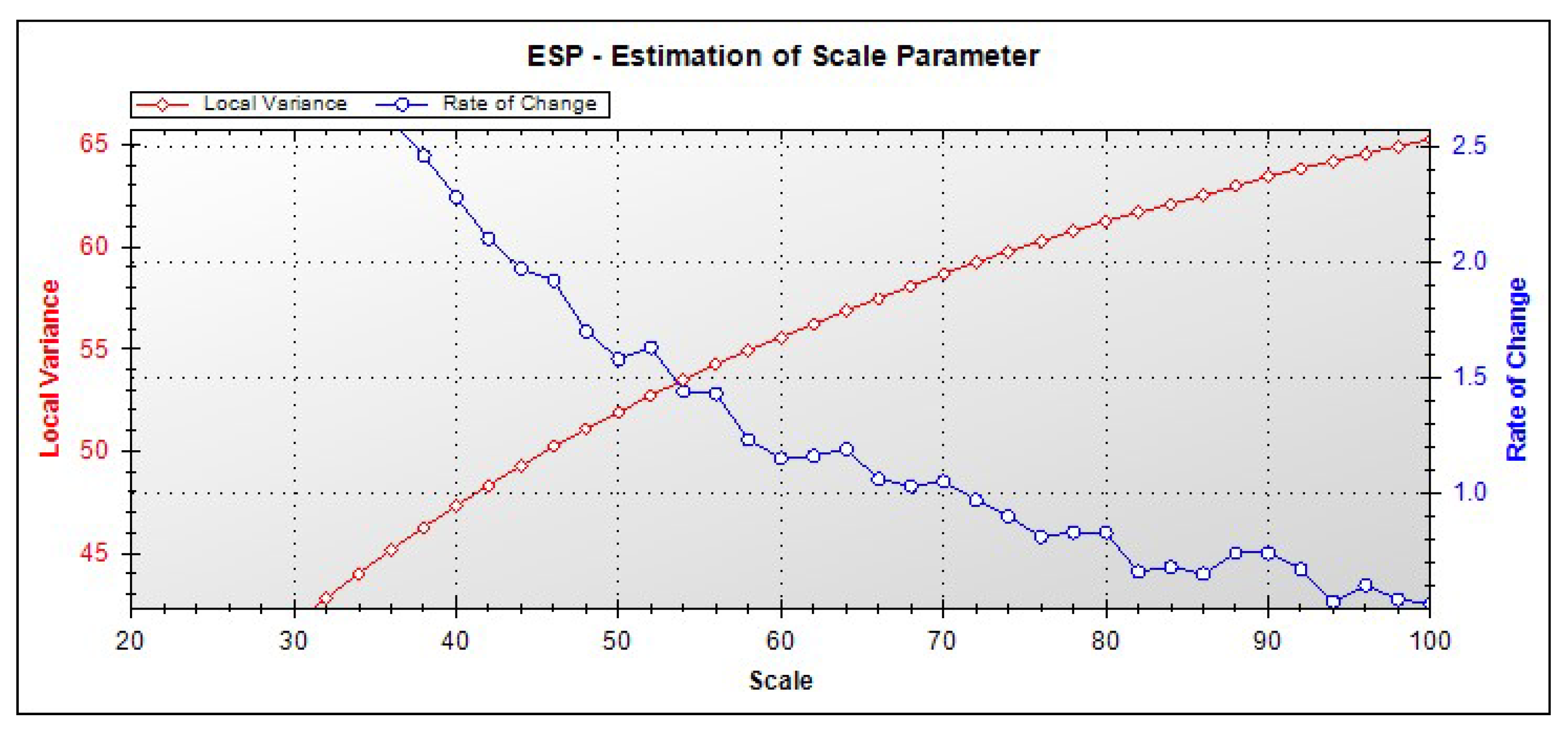
3.3. Object Segmentation and Integration with Pixel-Based Results
3.4. Accuracy Assessment
4. Results
4.1. Optical and SAR Image Composites
4.2. Corn Map of Hebei Province
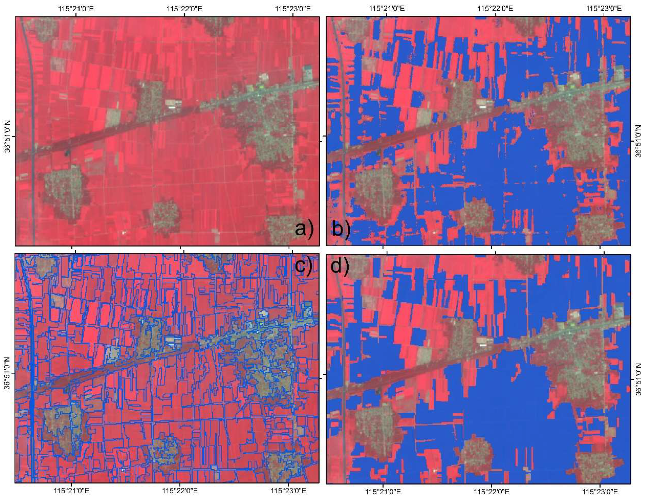
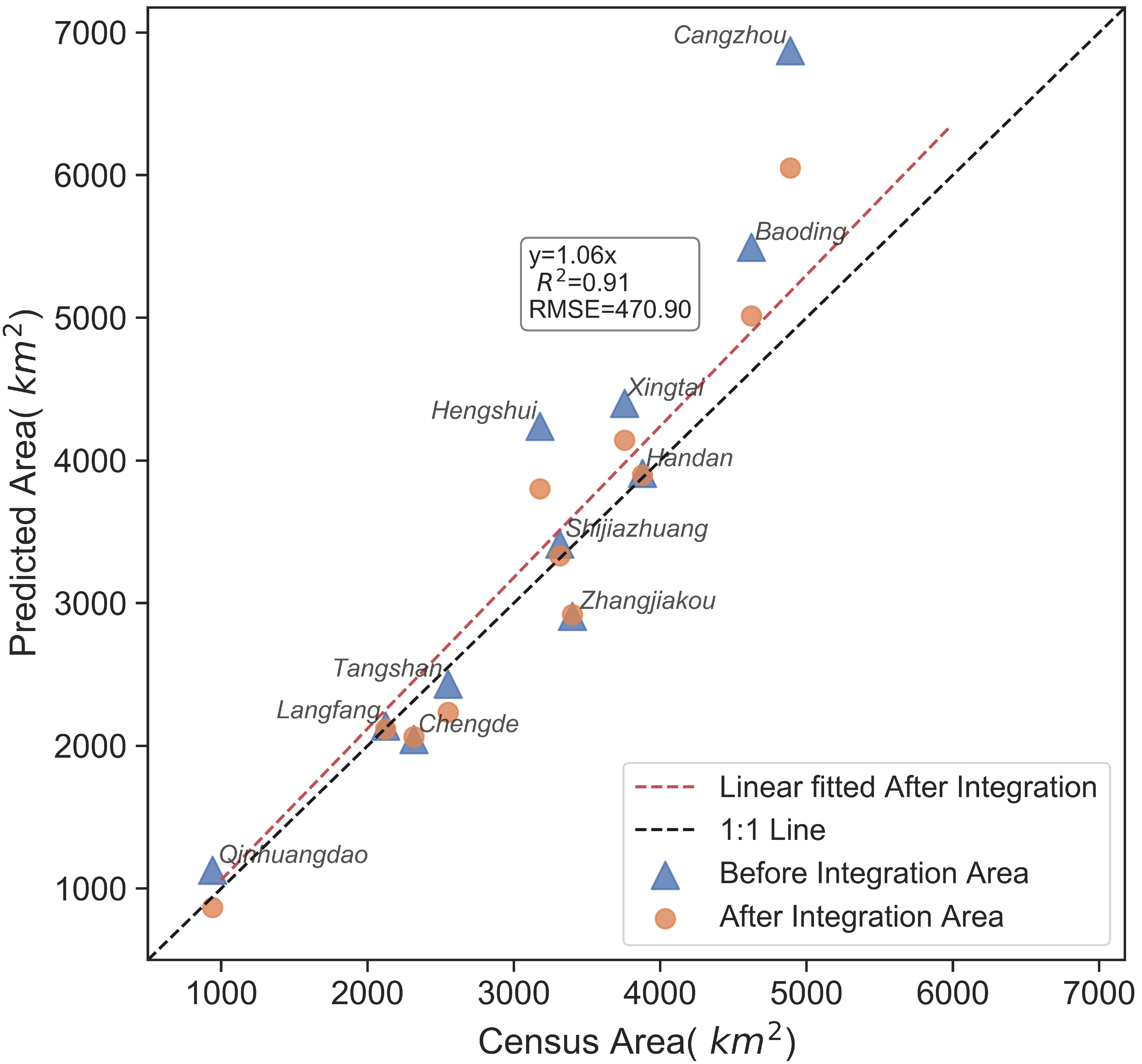
4.3. Comparison before and after Integration
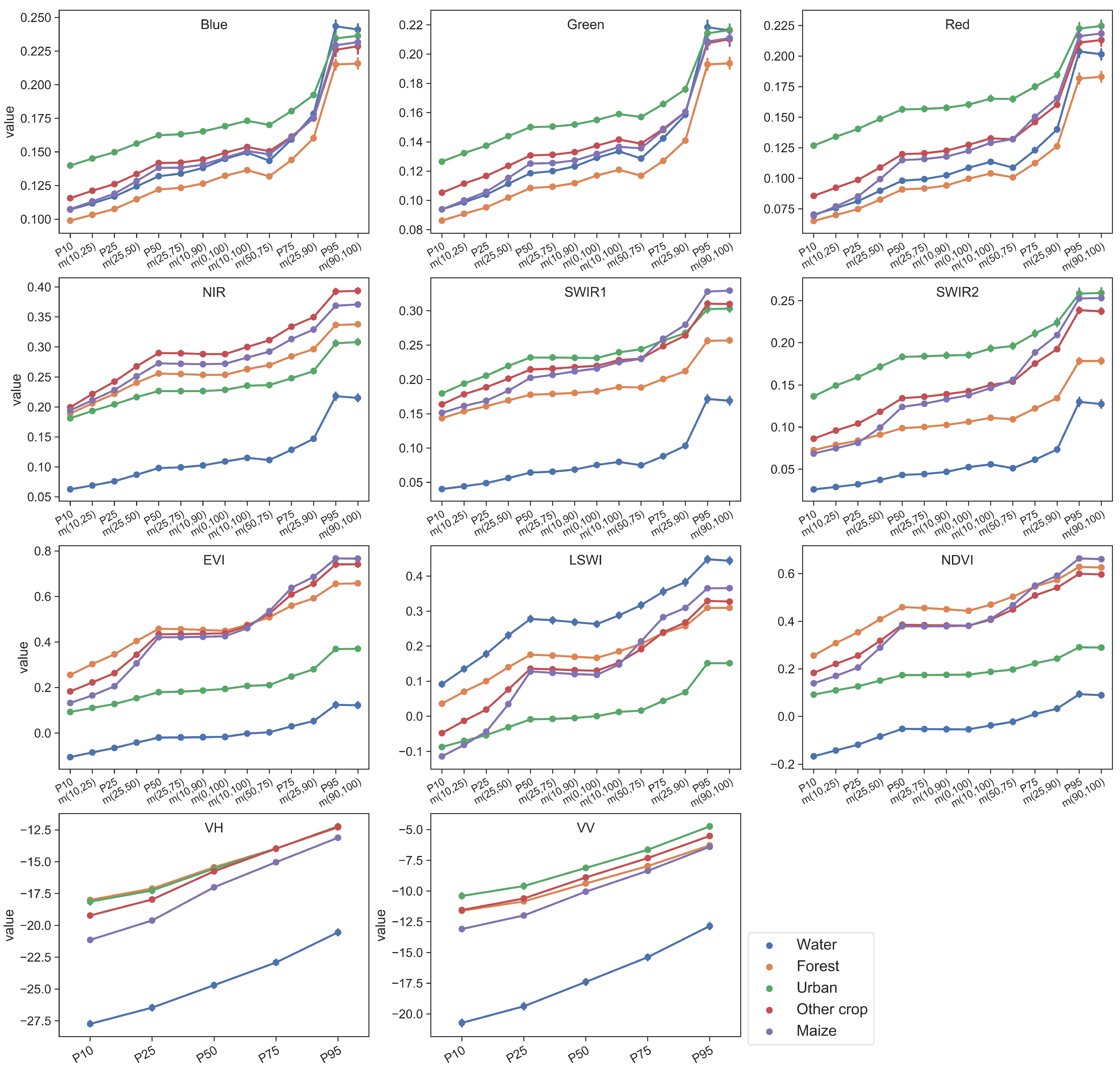
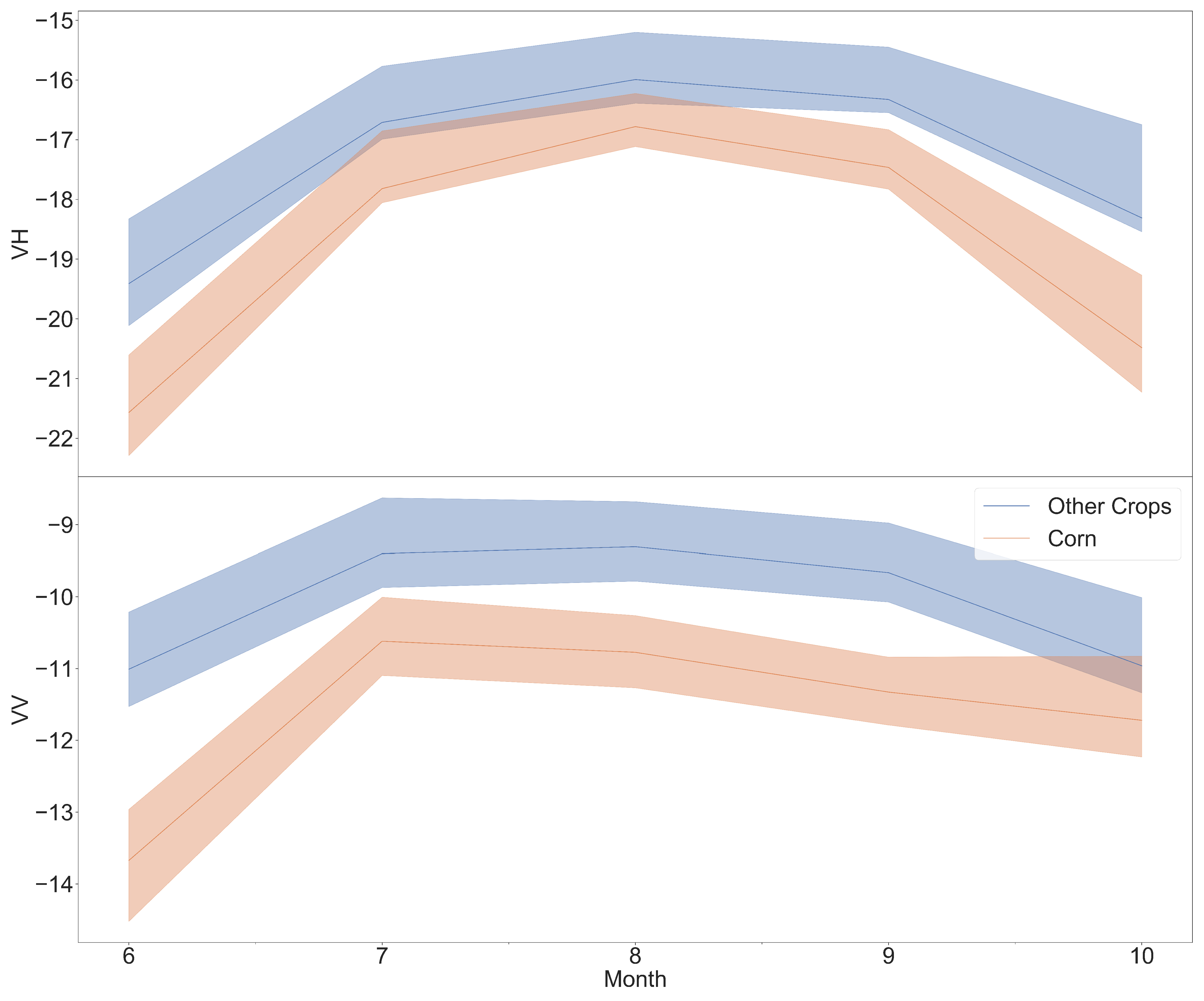
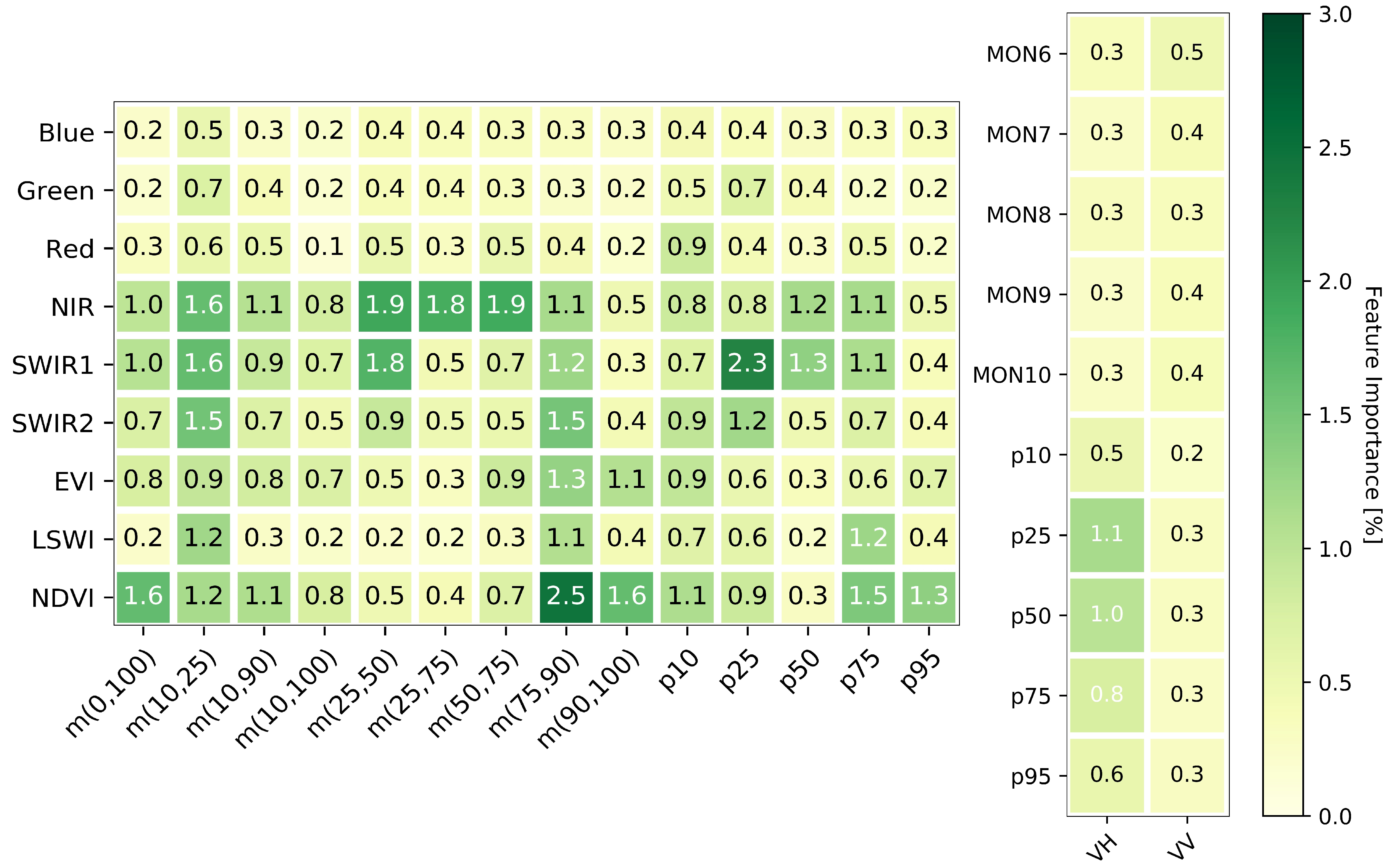
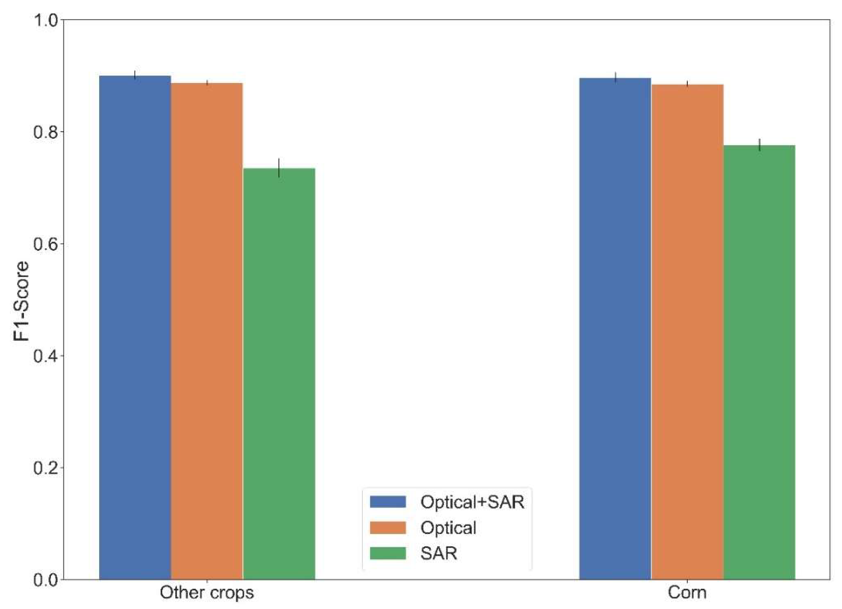
4.4. Contribution of the Features to Classification
5. Discussion
5.1. Reliability of Corn Mapping Using Optical and SAR Images in GEE
5.2. Uncertainty Analysis and Outlook
6. Conclusions
Author Contributions
Funding
Acknowledgments
Conflicts of Interest
References
- Zhang, X.; Wu, B.; Ponce-Campos, G.; Zhang, M.; Chang, S.; Tian, F. Mapping up-to-date paddy rice extent at 10 m resolution in china through the integration of optical and synthetic aperture radar images. Remote Sens. 2018, 10, 1200. [Google Scholar] [CrossRef]
- Zhong, L.; Gong, P.; Biging, G.S. Efficient corn and soybean mapping with temporal extendability: A multi-year experiment using landsat imagery. Remote Sens. Environ. 2014, 140, 1–13. [Google Scholar] [CrossRef]
- Griggs, D.; Stafford-Smith, M.; Gaffney, O.; Rockström, J.; Öhman, M.C.; Shyamsundar, P.; Steffen, W.; Glaser, G.; Kanie, N.; Noble, I. Policy: Sustainable development goals for people and planet. Nature 2013, 495, 305. [Google Scholar] [CrossRef]
- Wu, B.; Yan, N.; Xiong, J.; Bastiaanssen, W.G.M.; Zhu, W.; Stein, A. Validation of ETWatch using field measurements at diverse landscapes: A case study in Hai basin of china. J. Hydrol. 2012, 436–437, 67–80. [Google Scholar] [CrossRef]
- Yan, N.; Wu, B.; Perry, C.; Zeng, H. Assessing potential water savings in agriculture on the Hai basin plain, china. Agric. Water Manag. 2015, 154, 11–19. [Google Scholar] [CrossRef]
- Zhang, J.; Feng, L.; Yao, F. Improved maize cultivated area estimation over a large scale combining modis–evi time series data and crop phenological information. ISPRS J. Photogramm. Remote Sens. 2014, 94, 102–113. [Google Scholar] [CrossRef]
- Zwart, S.J.; Bastiaanssen, W.G.M. Review of measured crop water productivity values for irrigated wheat, rice, cotton and maize. Agric. Water Manag. 2004, 69, 115–133. [Google Scholar] [CrossRef]
- Song, X.-P.; Potapov, P.V.; Krylov, A.; King, L.; Di Bella, C.M.; Hudson, A.; Khan, A.; Adusei, B.; Stehman, S.V.; Hansen, M.C. National-scale soybean mapping and area estimation in the united states using medium resolution satellite imagery and field survey. Remote Sens. Environ. 2017, 190, 383–395. [Google Scholar] [CrossRef]
- Gao, F.; Anderson, M.C.; Zhang, X.; Yang, Z.; Alfieri, J.G.; Kustas, W.P.; Mueller, R.; Johnson, D.M.; Prueger, J.H. Toward mapping crop progress at field scales through fusion of landsat and MODIS imagery. Remote Sens. Environ. 2017, 188, 9–25. [Google Scholar] [CrossRef]
- Dong, J.; Xiao, X.; Menarguez, M.A.; Zhang, G.; Qin, Y.; Thau, D.; Biradar, C.; Moore, B., 3rd. Mapping paddy rice planting area in northeastern Asia with landsat 8 images, phenology-based algorithm and google earth engine. Remote Sens. Environ. 2016, 185, 142–154. [Google Scholar] [CrossRef]
- Wardlow, B.; Egbert, S.; Kastens, J. Analysis of time-series Modis 250 m vegetation index data for crop classification in the U.S. Central great plains. Remote Sens. Environ. 2007, 108, 290–310. [Google Scholar] [CrossRef]
- Wu, B.; Li, Q. Crop planting and type proportion method for crop acreage estimation of complex agricultural landscapes. Int. J. Appl. Earth Obs. Geoinf. 2012, 16, 101–112. [Google Scholar] [CrossRef]
- Immitzer, M.; Vuolo, F.; Atzberger, C. First experience with sentinel-2 data for crop and tree species classifications in central Europe. Remote Sens. 2016, 8, 166. [Google Scholar] [CrossRef]
- Zeng, L.; Wardlow, B.D.; Wang, R.; Shan, J.; Tadesse, T.; Hayes, M.J.; Li, D. A hybrid approach for detecting corn and soybean phenology with time-series MODIS data. Remote Sens. Environ. 2016, 181, 237–250. [Google Scholar] [CrossRef]
- Bargiel, D. A new method for crop classification combining time series of radar images and crop phenology information. Remote Sens. Environ. 2017, 198, 369–383. [Google Scholar] [CrossRef]
- Peña-Barragán, J.M.; Ngugi, M.K.; Plant, R.E.; Six, J. Object-based crop identification using multiple vegetation indices, textural features and crop phenology. Remote Sens. Environ. 2011, 115, 1301–1316. [Google Scholar] [CrossRef] [Green Version]
- Larrañaga, A.; Álvarez-Mozos, J. On the added value of Quad-Pol Data in a multi-temporal crop classification framework based on RADARSAT-2 imagery. Remote Sens. 2016, 8, 335. [Google Scholar] [CrossRef]
- Mascolo, L.; Lopez-Sanchez, J.M.; Vicente-Guijalba, F.; Nunziata, F.; Migliaccio, M.; Mazzarella, G. A complete procedure for crop phenology estimation with PolSAR data based on the complex Wishart classifier. IEEE Trans. Geosci. Remote Sens. 2016, 54, 6505–6515. [Google Scholar] [CrossRef]
- Wardlow, B.D.; Egbert, S.L. Large-area crop mapping using time-series MODIS 250 m NDVI data: An assessment for the U.S. Central great plains. Remote Sens. Environ. 2008, 112, 1096–1116. [Google Scholar] [CrossRef]
- Estel, S.; Kuemmerle, T.; Alcántara, C.; Levers, C.; Prishchepov, A.; Hostert, P. Mapping farmland abandonment and recultivation across Europe using MODIS NDVI time series. Remote Sens. Environ. 2015, 163, 312–325. [Google Scholar] [CrossRef]
- Pan, Z.; Huang, J.; Zhou, Q.; Wang, L.; Cheng, Y.; Zhang, H.; Blackburn, G.A.; Yan, J.; Liu, J. Mapping crop phenology using NDVI time-series derived from HJ-1 A/B data. Int. J. Appl. Earth Obs. Geoinf. 2015, 34, 188–197. [Google Scholar] [CrossRef] [Green Version]
- Estel, S.; Kuemmerle, T.; Levers, C.; Baumann, M.; Hostert, P. Mapping cropland-use intensity across Europe using MODIS NDVI time series. Environ. Res. Lett. 2016, 11, 024015. [Google Scholar] [CrossRef]
- Zhang, G.; Xiao, X.; Dong, J.; Kou, W.; Jin, C.; Qin, Y.; Zhou, Y.; Wang, J.; Menarguez, M.A.; Biradar, C. Mapping paddy rice planting areas through time series analysis of MODIS land surface temperature and vegetation index data. ISPRS J. Photogramm. Remote Sens. 2015, 106, 157–171. [Google Scholar] [CrossRef] [Green Version]
- Arvor, D.; Jonathan, M.; Meirelles, M.S.P.; Dubreuil, V.; Durieux, L. Classification of modis evi time series for crop mapping in the state of Mato Grosso, brazil. Int. J. Remote Sens. 2011, 32, 7847–7871. [Google Scholar] [CrossRef]
- Skakun, S.; Franch, B.; Vermote, E.; Roger, J.-C.; Becker-Reshef, I.; Justice, C.; Kussul, N. Early season large-area winter crop mapping using MODIS NDVI data, growing degree days information and a gaussian mixture model. Remote Sens. Environ. 2017, 195, 244–258. [Google Scholar] [CrossRef]
- Lee, E.; Kastens, J.H.; Egbert, S.L. Investigating collection 4 versus collection 5 MODIS 250 m NDVI time-series data for crop separability in Kansas, USA. Int. J. Remote Sens. 2016, 37, 341–355. [Google Scholar] [CrossRef]
- Massey, R.; Sankey, T.T.; Congalton, R.G.; Yadav, K.; Thenkabail, P.S.; Ozdogan, M.; Sánchez Meador, A.J. Modis phenology-derived, multi-year distribution of conterminous U.S. Crop types. Remote Sens. Environ. 2017, 198, 490–503. [Google Scholar] [CrossRef]
- Löw, F.; Prishchepov, A.; Waldner, F.; Dubovyk, O.; Akramkhanov, A.; Biradar, C.; Lamers, J. Mapping cropland abandonment in the Aral Sea Basin with MODIS time series. Remote Sens. 2018, 10, 159. [Google Scholar] [CrossRef]
- De Wit, A.J.W.; Clevers, J.G.P.W. Efficiency and accuracy of per-field classification for operational crop mapping. Int. J. Remote Sens. 2004, 25, 4091–4112. [Google Scholar] [CrossRef]
- Zheng, B.; Myint, S.W.; Thenkabail, P.S.; Aggarwal, R.M. A support vector machine to identify irrigated crop types using time-series Landsat NDVI data. Int. J. Appl. Earth Obs. Geoinf. 2015, 34, 103–112. [Google Scholar] [CrossRef]
- Vieira, M.A.; Formaggio, A.R.; Rennó, C.D.; Atzberger, C.; Aguiar, D.A.; Mello, M.P. Object based image analysis and data mining applied to a remotely sensed Landsat time-series to map sugarcane over large areas. Remote Sens. Environ. 2012, 123, 553–562. [Google Scholar] [CrossRef]
- Schultz, B.; Immitzer, M.; Formaggio, A.; Sanches, I.; Luiz, A.; Atzberger, C. Self-guided segmentation and classification of multi-temporal Landsat 8 images for crop type mapping in southeastern brazil. Remote Sens. 2015, 7, 14482–14508. [Google Scholar] [CrossRef]
- Kontgis, C.; Schneider, A.; Ozdogan, M. Mapping rice paddy extent and intensification in the vietnamese mekong river delta with dense time stacks of Landsat data. Remote Sens. Environ. 2015, 169, 255–269. [Google Scholar] [CrossRef]
- Bontemps, S.; Arias, M.; Cara, C.; Dedieu, G.; Guzzonato, E.; Hagolle, O.; Inglada, J.; Matton, N.; Morin, D.; Popescu, R.; et al. Building a data set over 12 globally distributed sites to support the development of agriculture monitoring applications with sentinel-2. Remote Sens. 2015, 7, 16062–16090. [Google Scholar] [CrossRef]
- Inglada, J.; Arias, M.; Tardy, B.; Hagolle, O.; Valero, S.; Morin, D.; Dedieu, G.; Sepulcre, G.; Bontemps, S.; Defourny, P.; et al. Assessment of an operational system for crop type map production using high temporal and spatial resolution satellite optical imagery. Remote Sens. 2015, 7, 12356–12379. [Google Scholar] [CrossRef]
- Matton, N.; Canto, G.; Waldner, F.; Valero, S.; Morin, D.; Inglada, J.; Arias, M.; Bontemps, S.; Koetz, B.; Defourny, P. An automated method for annual cropland mapping along the season for various globally-distributed agrosystems using high spatial and temporal resolution time series. Remote Sens. 2015, 7, 13208–13232. [Google Scholar] [CrossRef]
- Valero, S.; Morin, D.; Inglada, J.; Sepulcre, G.; Arias, M.; Hagolle, O.; Dedieu, G.; Bontemps, S.; Defourny, P.; Koetz, B. Production of a dynamic cropland mask by processing remote sensing image series at high temporal and spatial resolutions. Remote Sens. 2016, 8, 55. [Google Scholar] [CrossRef]
- Skriver, H. Crop classification by multitemporal C- and L-band single- and dual-polarization and fully polarimetric SAR. IEEE Trans. Geosci. Remote Sens. 2012, 50, 2138–2149. [Google Scholar] [CrossRef]
- Freeman, A.; Villasenor, J.; Klein, J.; Hoogeboom, P.; Groot, J. On the use of multi-frequency and polarimetric radar backscatter features for classification of agricultural crops. Int. J. Remote Sens. 1994, 15, 1799–1812. [Google Scholar] [CrossRef]
- Schmullius, C.; Schrage, T. Classification, Crop Parameter Estimation and Synergy Effects Using Airborne DLR E-SAR and DAEDALUS Images. In Proceedings of the 1998 IEEE International Geoscience and Remote Sensing Symposium, IGARSS’98, Seattle, WA, USA, 6–10 July 1998; pp. 97–99. [Google Scholar]
- Lee, J.-S.; Grunes, M.R.; Pottier, E. Quantitative comparison of classification capability: Fully polarimetric versus dual and single-polarization SAR. IEEE Trans. Geosci. Remote Sens. 2001, 39, 2343–2351. [Google Scholar]
- Del Frate, F.; Schiavon, G.; Solimini, D.; Borgeaud, M.; Hoekman, D.H.; Vissers, M.A. Crop classification using multiconfiguration C-band SAR data. IEEE Trans. Geosci. Remote Sens. 2003, 41, 1611–1619. [Google Scholar] [CrossRef]
- Jia, K.; Li, Q.; Tian, Y.; Wu, B.; Zhang, F.; Meng, J. Crop classification using multi-configuration SAR data in the north china plain. Int. J. Remote Sens. 2011, 33, 170–183. [Google Scholar] [CrossRef]
- McNairn, H.; Shang, J.; Jiao, X.; Champagne, C. The contribution of ALOS PALSAR multipolarization and polarimetric data to crop classification. IEEE Trans. Geosci. Remote Sens. 2009, 47, 3981–3992. [Google Scholar] [CrossRef]
- Gorelick, N.; Hancher, M.; Dixon, M.; Ilyushchenko, S.; Thau, D.; Moore, R. Google earth engine: Planetary-scale geospatial analysis for everyone. Remote Sens. Environ. 2017, 202, 18–27. [Google Scholar] [CrossRef]
- Hansen, M.C.; Potapov, P.V.; Moore, R.; Hancher, M.; Turubanova, S.; Tyukavina, A.; Thau, D.; Stehman, S.; Goetz, S.; Loveland, T. High-resolution global maps of 21st-century forest cover change. Science 2013, 342, 850–853. [Google Scholar] [CrossRef]
- Patel, N.N.; Angiuli, E.; Gamba, P.; Gaughan, A.; Lisini, G.; Stevens, F.R.; Tatem, A.J.; Trianni, G. Multitemporal settlement and population mapping from Landsat using google earth engine. Int. J. Appl. Earth Obs. Geoinf. 2015, 35, 199–208. [Google Scholar] [CrossRef]
- Xiong, J.; Thenkabail, P.S.; Gumma, M.K.; Teluguntla, P.; Poehnelt, J.; Congalton, R.G.; Yadav, K.; Thau, D. Automated cropland mapping of continental Africa using google earth engine cloud computing. ISPRS J. Photogramm. Remote Sens. 2017, 126, 225–244. [Google Scholar] [CrossRef]
- Goldblatt, R.; You, W.; Hanson, G.; Khandelwal, A. Detecting the boundaries of urban areas in india: A dataset for pixel-based image classification in google earth engine. Remote Sens. 2016, 8, 634. [Google Scholar] [CrossRef]
- Azzari, G.; Lobell, D.B. Landsat-based classification in the cloud: An opportunity for a paradigm shift in land cover monitoring. Remote Sens. Environ. 2017, 202, 64–74. [Google Scholar] [CrossRef]
- Huang, H.; Chen, Y.; Clinton, N.; Wang, J.; Wang, X.; Liu, C.; Gong, P.; Yang, J.; Bai, Y.; Zheng, Y.; et al. Mapping major land cover dynamics in Beijing using all Landsat images in google earth engine. Remote Sens. Environ. 2017, 202, 166–176. [Google Scholar] [CrossRef]
- National Bureau of Statistics of China. National Data. Available online: http://data.stats.gov.cn/easyquery.htm?cn=E0103&zb=A0D0P®=130000&sj=2016 (accessed on 22 October 2018).
- Cai, Y.; Guan, K.; Peng, J.; Wang, S.; Seifert, C.; Wardlow, B.; Li, Z. A high-performance and in-season classification system of field-level crop types using time-series Landsat data and a machine learning approach. Remote Sens. Environ. 2018, 210, 35–47. [Google Scholar] [CrossRef]
- Tucker, C.J. Red and photographic infrared linear combinations for monitoring vegetation. Remote Sens. Environ. 1979, 8, 127–150. [Google Scholar] [CrossRef] [Green Version]
- Huete, A.; Didan, K.; Miura, T.; Rodriguez, E.P.; Gao, X.; Ferreira, L.G. Overview of the radiometric and biophysical performance of the MODIS vegetation indices. Remote Sen. Environ. 2002, 83, 195–213. [Google Scholar] [CrossRef]
- Xiao, X.; Boles, S.; Liu, J.; Zhuang, D.; Liu, M. Characterization of forest types in Northeastern China, using multi-temporal spot-4 vegetation sensor data. Remote Sens. Environ. 2002, 82, 335–348. [Google Scholar] [CrossRef]
- Sellers, P.; Berry, J.; Collatz, G.; Field, C.; Hall, F. Canopy reflectance, photosynthesis, and transpiration. III. A reanalysis using improved leaf models and a new canopy integration scheme. Remote Sens. Environ. 1992, 42, 187–216. [Google Scholar] [CrossRef]
- Veci, L. Sentinel-1 Toolbox; SAR Basics Tutoria; Array Systems Computing Inc.: North York, ON, Canada, 2016. [Google Scholar]
- RADI. Gvg for Android. Available online: https://play.google.com/store/apps/details?id=com.sysapk.gvg&hl=en_US (accessed on 29 October 2018).
- Benediktsson, J.A.; Swain, P.H.; Ersoy, O.K. Neural network approaches versus statistical methods in classification of multisource remote sensing data. In Proceedings of the 12th Canadian Symposium on Remote Sensing Geoscience and Remote Sensing Symposium, Vancouver, BC, Canada, 6–10 July 1990. [Google Scholar]
- Blaschke, T. Object based image analysis for remote sensing. ISPRS J. Photogramm. Remote Sens. 2010, 65, 2–16. [Google Scholar] [CrossRef] [Green Version]
- Potapov, P.V.; Turubanova, S.A.; Hansen, M.C.; Adusei, B.; Broich, M.; Altstatt, A.; Mane, L.; Justice, C.O. Quantifying forest cover loss in democratic republic of the Congo, 2000–2010, with Landsat ETM+ data. Remote Sens. Environ. 2012, 122, 106–116. [Google Scholar] [CrossRef]
- Breiman, L. Random forests. Mach. Learn. 2001, 45, 5–32. [Google Scholar] [CrossRef]
- Belgiu, M.; Drăguţ, L. Random forest in remote sensing: A review of applications and future directions. ISPRS J. Photogramm. Remote Sens. 2016, 114, 24–31. [Google Scholar] [CrossRef]
- Yan, J.; Lin, L.; Zhou, W.; Ma, K.; Pickett, S.T.A. A novel approach for quantifying particulate matter distribution on leaf surface by combining SEM and object-based image analysis. Remote Sens. Environ. 2016, 173, 156–161. [Google Scholar] [CrossRef] [Green Version]
- Lu, M.; Chen, J.; Tang, H.; Rao, Y.; Yang, P.; Wu, W. Land cover change detection by integrating object-based data blending model of Landsat and MODIS. Remote Sens. Environ. 2016, 184, 374–386. [Google Scholar] [CrossRef]
- Drǎguţ, L.; Tiede, D.; Levick, S.R. Esp: A tool to estimate scale parameter for multiresolution image segmentation of remotely sensed data. Int. J. Geogr. Inf. Sci. 2010, 24, 859–871. [Google Scholar] [CrossRef]
- Dragut, L.; Csillik, O.; Eisank, C.; Tiede, D. Automated parameterisation for multi-scale image segmentation on multiple layers. ISPRS J. Photogramm. Remote Sens. 2014, 88, 119–127. [Google Scholar] [CrossRef] [Green Version]
- National Bureau of Statistics of China. National Data. Available online: http://data.stats.gov.cn/english/easyquery.htm?cn=E0103 (accessed on 11 March 2018).
- Pedregosa, F.; Varoquaux, G.; Gramfort, A.; Michel, V.; Thirion, B.; Grisel, O.; Blondel, M.; Prettenhofer, P.; Weiss, R.; Dubourg, V. Scikit-learn: Machine learning in python. J. Mach. Learn. Res. 2011, 12, 2825–2830. [Google Scholar]
- Ghulam, A.; Li, Z.-L.; Qin, Q.; Yimit, H.; Wang, J. Estimating crop water stress with ETM+ NIR and SWIR data. Agric. For. Meteorol. 2008, 148, 1679–1695. [Google Scholar] [CrossRef]
- You, J.; Li, X.; Low, M.; Lobell, D.; Ermon, S. Deep gaussian process for crop yield prediction based on remote sensing data. In Proceedings of the Thirty-First AAAI Conference on Artificial Intelligence, AAAI, San Francisco, CA, USA, 4–9 February 2017; pp. 4559–4566. [Google Scholar]
- ESA. First Sentinel-2B Images Delivered by Laser. Available online: https://www.esa.int/Our_Activities/Observing_the_Earth/Copernicus/Sentinel-2/First_Sentinel-2B_images_delivered_by_laser (accessed on 11 December 2018).
- Massey, R.; Sankey, T.T.; Yadav, K.; Congalton, R.G.; Tilton, J.C. Integrating cloud-based workflows in continental-scale cropland extent classification. Remote Sens. Environ. 2018, 219, 162–179. [Google Scholar] [CrossRef]
- Sundermeyer, M.; Schlüter, R.; Ney, H. Lstm neural networks for language modeling. In Proceedings of the Thirteenth Annual Conference of the International Speech Communication Association, Portland, OR, USA, 9–13 September 2012. [Google Scholar]
- RuBwurm, M.; Körner, M. Temporal vegetation modelling using long short-term memory networks for crop identification from medium-resolution multi-spectral satellite images. In Proceedings of the CVPR Workshops, Honolulu, HI, USA, 21–26 July 2017; pp. 1496–1504. [Google Scholar]


| Hebei Province | Map Data | ||||
|---|---|---|---|---|---|
| Other Crops | Corn | Total | Producer’s Accuracy | ||
| Field data | Other Crops | 784 | 86 | 870 | 90.11% |
| Corn | 94 | 817 | 911 | 89.68% | |
| Total | 878 | 903 | 1781 | ||
| User’s Accuracy | 89.29% | 90.48% | |||
| F1-Score | 89.70% | 90.08% | Overall Accuracy | 89.89% | |
| Region | Crop | Producer’s Accuracy | User’s Accuracy | F1-Score |
|---|---|---|---|---|
| Baoding | Other Crops | 82.05% | 74.42% | 78.05% |
| Corn | 92.57% | 95.14% | 93.84% | |
| Cangzhou | Other Crops | 87.72% | 92.59% | 90.09% |
| Corn | 96.40% | 93.86% | 95.11% | |
| Chengde | Other Crops | 86.67% | 90.28% | 88.44% |
| Corn | 86.27% | 81.48% | 83.81% | |
| Handan | Other Crops | 92.31% | 94.12% | 93.20% |
| Corn | 88.10% | 84.73% | 86.38% | |
| Hengshui | Other Crops | 85.81% | 86.93% | 86.36% |
| Corn | 88.57% | 87.57% | 88.07% | |
| Langfang | Other Crops | 97.92% | 92.16% | 94.95% |
| Corn | 91.49% | 97.73% | 94.51% | |
| Qinhuangdao | Other Crops | 80.36% | 90.00% | 84.91% |
| Corn | 90.20% | 80.70% | 85.19% | |
| Shijiazhuang | Other Crops | 84.85% | 93.33% | 88.89% |
| Corn | 89.47% | 77.27% | 82.93% | |
| Tangshan | Other Crops | 90.91% | 90.91% | 90.91% |
| Corn | 90.00% | 90.00% | 90.00% | |
| Xingtai | Other Crops | 95.38% | 83.22% | 88.89% |
| Corn | 79.51% | 94.17% | 86.22% | |
| Zhangjiakou | Other Crops | 90.00% | 96.43% | 93.10% |
| Corn | 93.75% | 83.33% | 88.24% |
© 2019 by the authors. Licensee MDPI, Basel, Switzerland. This article is an open access article distributed under the terms and conditions of the Creative Commons Attribution (CC BY) license (http://creativecommons.org/licenses/by/4.0/).
Share and Cite
Tian, F.; Wu, B.; Zeng, H.; Zhang, X.; Xu, J. Efficient Identification of Corn Cultivation Area with Multitemporal Synthetic Aperture Radar and Optical Images in the Google Earth Engine Cloud Platform. Remote Sens. 2019, 11, 629. https://doi.org/10.3390/rs11060629
Tian F, Wu B, Zeng H, Zhang X, Xu J. Efficient Identification of Corn Cultivation Area with Multitemporal Synthetic Aperture Radar and Optical Images in the Google Earth Engine Cloud Platform. Remote Sensing. 2019; 11(6):629. https://doi.org/10.3390/rs11060629
Chicago/Turabian StyleTian, Fuyou, Bingfang Wu, Hongwei Zeng, Xin Zhang, and Jiaming Xu. 2019. "Efficient Identification of Corn Cultivation Area with Multitemporal Synthetic Aperture Radar and Optical Images in the Google Earth Engine Cloud Platform" Remote Sensing 11, no. 6: 629. https://doi.org/10.3390/rs11060629