Monitoring and Analyzing Mountain Glacier Surface Movement Using SAR Data and a Terrestrial Laser Scanner: A Case Study of the Himalayas North Slope Glacier Area

Abstract

The offset tracking technique based on synthetic aperture radar (SAR) image intensity information can estimate glacier displacement even when glacier velocities are high and the time interval between images is long, allowing for the broad use of this technique in glacier velocity monitoring. Terrestrial laser scanners, a non-contact measuring system, can measure the velocity of a glacier even if there are no control points arranged on a glacier. In this study, six COSMO-SkyMed images acquired between 31 July and 22 December 2016 were used to obtain the glacial movements of five glaciers on the northern slope of the central Himalayas using the offset tracking approach. During the period of image acquirement, a terrestrial laser scanner was used, and point clouds of two periods in a small area at the terminus of the Pingcuoliesa Glacier were obtained. By selecting three fixed areas of the point clouds that have similar shapes across two periods, the displacements of the centers of gravity of the selected areas were calculated by using contrast analyses of feature points. Although the overall low-density point clouds data indicate that the glacial surfaces have low albedos relative to the wavelength of the terrestrial laser scanner and the effect of its application is therefore influenced in this research, the registration accuracy of 0.0023 m/d in the non-glacial areas of the scanner’s measurements is acceptable, considering the magnitude of 0.072 m/d of the minimum glacial velocity measured by the scanner. The displacements from the point clouds broadly agree with the results of the offset tracking technique in the same area, which provides further evidence of the reliability of the measurements of the SAR data in addition to the analyses of the root mean squared error of the velocity residuals in non-glacial areas. The analysis of the movement of five glaciers in the study area revealed the dynamic behavior of these glacial surfaces across five periods. G089972E28213N Glacier, Pingcuoliesa Glacier and Shimo Glacier show increasing surface movement velocities from the terminus end to the upper part with elevations of 1500 m, 4500 m, and 6400 m, respectively. The maximum velocities on the glacial surface profiles were 31.69 cm/d, 62.40 cm/d, and 42.00 cm/d, respectively. In contrast, the maximum velocity of Shie Glacier, 50.60 cm/d, was observed at the glacier’s terminus. For each period, G090138E28210N Glacier exhibited similar velocity values across the surface profile, with a maximum velocity of 39.70 cm/d. The maximum velocities of G089972E28213N Glacier, Pingcuoliesa Glacier, and Shie Glacier occur in the areas where the topography is steepest. In general, glacial surface velocities are higher in the summer than in the winter in this region. With the assistance of a terrestrial laser scanner with optimized wavelengths or other proper ground-based remote sensing instruments, the offset tracking technique based on high-resolution satellite SAR data should provide more reliable and detailed information for local and even single glacial surface displacement monitoring.

1. Introduction

Glacial movement is an important component of glaciology that is influenced by the mass balance, temperature, and hydraulic characteristics of glaciers [1,2]. Over long periods of time, glacial velocity depends on both terrain and climate [2]. Thus, glacial movement velocity can provide valuable insights into changes in climate conditions. Mountain glaciers, which are mainly distributed across Asia and North America, are important freshwater resources. However, mountain glaciers may also pose serious risks to the safety of human settlements downstream due to the possibility of glacial lake outburst floods and debris flows caused by glacial movement [3]. In Chinese Tibet alone, there have been 27 known glacial lake outbursts since the 1930s, which have resulted in tremendous losses of life, property, and infrastructure in the adjacent downstream areas [4]. Moreover, the frequency, scale, and consequences of glacial disasters have been increasing, resulting in great concern for downstream municipalities. The monitoring of glacial movement, especially the movement of glaciers connected to lakes, is of both academic and practical importance.

Due to the remote locations and difficult environments in which many mountain glaciers are found, monitoring their velocity in situ is time-consuming and costly, making it difficult to conduct regular observations. The launch of remote sensing satellites, especially synthetic aperture radar (SAR) satellites, has made it possible to monitor the surface movement of glaciers regularly and across large spatial scales [5,6,7,8,9,10]. Based on SAR images, differential interferometric SAR (DInSAR) was first used by Goldstein et al. to extract the displacement of the Rutford Ice Stream in Antarctica with centimeter-level accuracy in 1993 [11]. Since then, more scholars have developed new techniques and methods for monitoring glacial velocity using SAR data. To solve the limitation that DInSAR can only estimate light-of-sight deformation, Gray et al. presented a SAR image registration method that can extract displacements in the azimuth and range directions of glaciers [12]. Based on the intensity information of SAR images, this method, which can be called the offset tracking technique (or speckle tracking technique), is better able to resist decorrelation [13,14,15]. Another SAR method, proposed by Bechor et al. in 2006, is multi-aperture interferometry (MAI), which utilizes the phase information of SAR images similarly to DInSAR, providing a way to extract high-accuracy displacements in azimuth direction [16]. Overall, both DInSAR and MAI can achieve centimeter-scale precision, which is ultimately limited by the high coherence of SAR images. The accuracy of the offset tracking technique is generally 1/10- to 1/30-pixel size, and it is generally more robust. Moreover, SAR image resolution is now possible at a scale of <1 m, thus, the offset tracking technique allows for sub-decimeter accuracy [17].

The reliability of glacial velocity results based on SAR images is typically validated by calculating the velocity residuals of the bedrock area [18,19,20]. To conduct further validation, some scholars also employ photogrammetric forward intersection, differential GPS (DGPS), and other validation methods to measure the velocity of points on a glacial surface [21,22,23,24]. However, it is necessary to place markers on the surface of glaciers, which is often difficult to implement because of the harsh environments there. An alternative non-contact measurement system is the 3D laser scanner, which can quickly obtain high-precision and high-density point clouds of the scanned area over several kilometers [25]. By scanning the study area multiple times and comparing the spatial distribution of resulting point clouds, the deformation of the study area can be measured [26], allowing for complementary verification of the measurements made via SAR data.

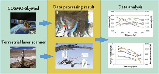
In this paper, six COSMO-SkyMed images were processed using the offset tracking technique to extract the glacial velocity on the northern slope of the Himalayas. A supplementary measurement instrument, a terrestrial laser scanner, was used to acquire the velocity of part of the Pingcuoliesa Glacier. By comparing nearly contemporaneous displacements estimated by point clouds and SAR images, the potential and reliability of both the terrestrial laser scanner and offset tracking technique for monitoring the velocity of mountain glaciers were evaluated. Thanks to the high resolution of the SAR images, the detailed surface movement characteristics of five mountain glaciers in this the study area were analyzed.

2. Study Area and Datasets

2.1. Study Area

The study area is located on the northern slope of the central Himalayas between Kangma County and Langkazi County in Tibet of China, covering the geographic area between ~28°07′~−28°19′N and ~89°53′–90°22′E. The average elevation of the region (shown in the Figure 1) is about 5000 m, and the difference in elevation is over 2000 m. In the study area, there are two large glacial lakes: Shie and Shimo. Shie Lake, the largest glacial lake in the Himalayas, is about 5.695 million square meters in area, and it is the source of the Nyang Qu. In 1954, Shie Lake had an outburst, resulting in the deaths of 400 people and impacting 20,000 other people.

2.2. SAR Data

The COSMO-SkyMed Earth Observing System contains four X-band (9.6 GHz) SAR satellites with multiple imaging modes, and can acquire interferometric image pairs at 1-, 3-, 4-, and 8-day intervals [17]. The COSMO-SkyMed images used in this study were acquired in HImage scanning mode with 3 m resolution, HH polarization, and a descending pass. The combination of images is shown in

Table 1. Pairs of COSMO-SkyMed SAR data.

Master Image	Slave Image	Perpendicular Baseline(m)	Time Baseline(d)
2016/07/31	2016/08/01	−213.3	1
2016/07/31	2016/08/16	613.2	16
2016/08/16	2016/09/21	125.3	36
2016/09/21	2016/10/07	118.8	16
2016/10/07	2016/10/19	−673.1	12
2016/10/19	2016/12/22	101.7	64

. The NASA Shuttle Radar Topographic Mission digital elevation model (SRTM-DEM) data used by this paper have a resolution of about 30 m × 30 m [28].

2.3. Collection of Point Clouds Data on Glacial Surfaces

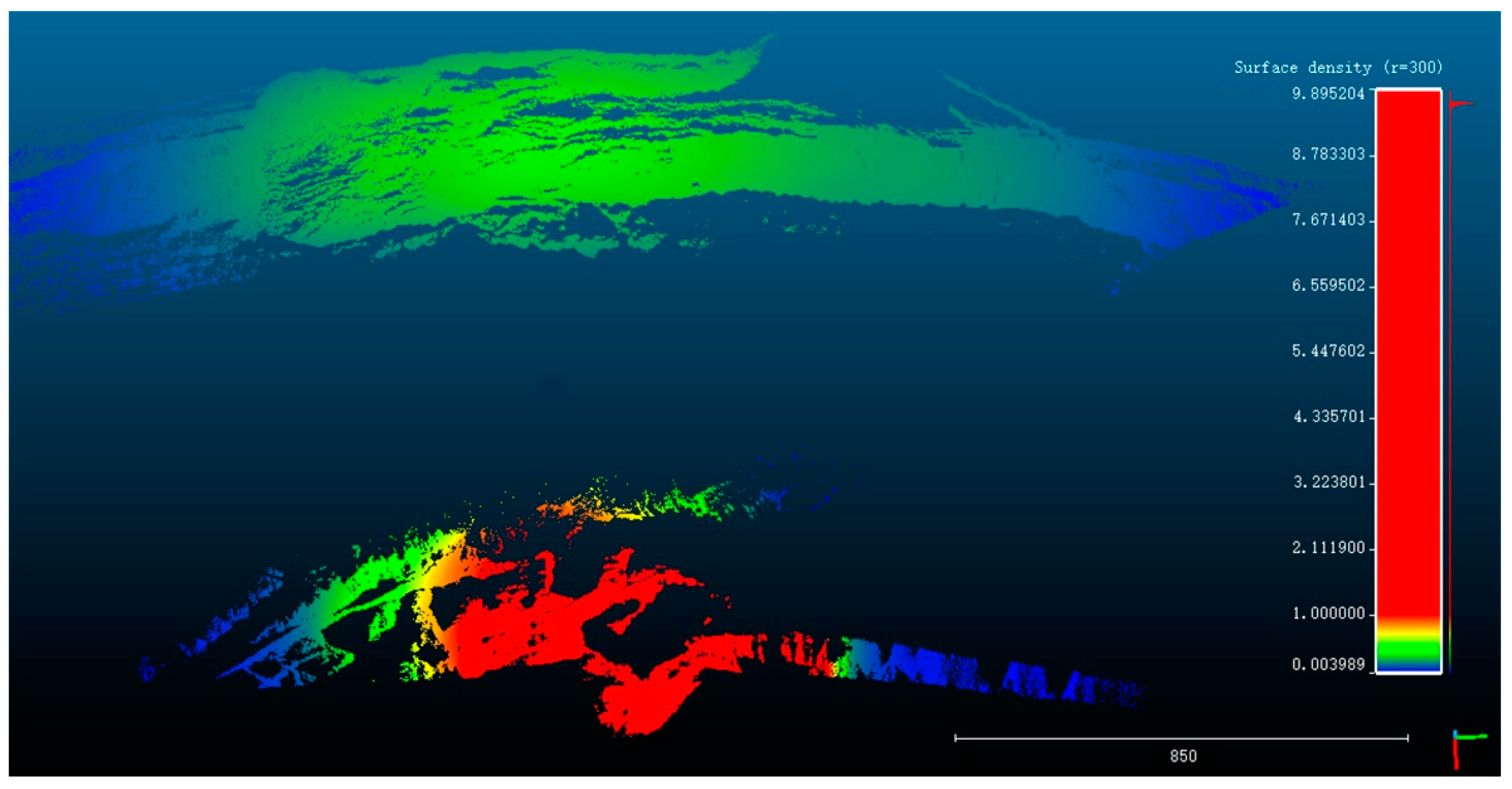
The study area is in a harsh environment with low oxygen content and steep terrain, making it difficult to place markers on the glacial surface. After a field survey, a terrestrial laser scanner was placed on the east side of the Pingcuoliesa Glacier (Figure 1). The terrestrial laser scanner is a RIEGL LMS-Z620, which consists of a 3D scanner with a 2-km measuring range, RiSCAN PRO operating and data processing software, and a calibrated high-resolution professional digital SLR camera. The location of the selected 3D laser scanner was fixed at 28.265833° latitude and 89.998056° longitude; the altitude was 5223 m. To ensure accurate point clouds registration as well as to geocode the point clouds to the geographic coordinate system, five retro-reflective targets were placed near the site as control points, and the latitude and longitude coordinates of the target were measured by GPS. During the acquisition period of COSMO-SkyMed images from 21 September to 7 October 2016, two point clouds datasets were acquired on-site using the terrestrial laser scanner at 13:10 on 29 September 2016 and 13:30 on 5 October 2016. The scanning resolution is set to 2 cm, which results in 2-cm resolution of the point clouds at short distances. In this paper, it is found that the short distance is about 10 m by analyzing a density figure of the point clouds. The density figure of the point clouds at 13:10 on 29 September 2016 is shown as Figure 2, where the surface density is estimated by counting the number of points in an area with radius of 300 m.

To study the relationship between the glacial surface velocity and temperature change, daily average temperature data in Kangma County were obtained for 31 July 2016 to 22 December 2016 from the weather website (lishi.tianqi.com). The data published on the website come from the China Meteorological Administration.

2.4. Temperature Data

To study the relationship between the glacial surface velocity and temperature change, daily average temperature data in Kangma County were obtained for 31 July 2016 to 22 December 2016 from the weather website (lishi.tianqi.com). The data published on the website come from the China Meteorological Administration.

3. Methods and Data Processing

3.1. Offset Tracking Technique Applied to SAR Data

Differential interferogram and coherence map were generated via DInSAR for two COSMO-SkyMed images acquired on 31 July and 1 August 2016 with 1-day time intervals. No deformation fringe was found in the glacial region, and coherence was very low. According to the temperature data in the study area, the daily average temperature was almost always above zero degrees Celsius during the observation (Figure 3). In August, the temperature even reached ten degrees Celsius, which caused the surface of the glacier to melt, changing the glacier surface conditions slightly. Thus, decorrelation occurred on the surface of the glacier. Both the DInSAR and MAI techniques, which are based on the phase information of SAR images, are limited for the SAR data used in this paper (Figure 4), while the offset tracking technique based on the intensity information can be used in the areas with no coherence. Therefore, the offset tracking technique and high-resolution SAR images were used to estimate the glacial velocity in this study.

The offset tracking technique calculates the offset of the corresponding pixel of two SAR images based on the normalized cross-correlation algorithm. The normalized cross-correlation algorithm determines the matching degree by calculating the cross-correlation coefficient $C{C}_{\left(L,S\right)}$ between the template window in the reference image and the search window in the co-registered image. The value of $C{C}_{\left(L,S\right)}$ reflects the similarity between the template window and the search window. When the $C{C}_{\left(L,S\right)}$ is maximized, the match between the template window and the search window is completed, and the pixel offset between the two SAR images is calculated [24,29,30,31].

$$C{C}_{(L,S)}=\frac{{\sum }_{(l,s)}(r_{(l,s)}-{\mu }_r)(s_{(l,s)}-{\mu }_s)}{{[{\sum }_{(l,s)}{(r_{(l,s)}-{\mu }_r)}^2]}^{1/2}{[{\sum }_{(l,s)}{(s_{(l,s)}-{\mu }_s)}^2]}^{1/2}}$$

In general, pixel offsets consist of offsets caused by orbital differences, glacial motion, topography, and the ionosphere [32]. The global offset due to orbital differences can be removed by polynomial fitting, in this paper, the non-glacial area is used to estimate the overall co-registration parameter, and there is no related systematic error in the offset results [29,30]. The ionosphere has a negligible influence on X-band images in low-, and mid-latitude areas and can thus be ignored [33]. The offset caused by topography is proportional to the perpendicular baseline and the altitude difference in the slant-range direction, and it is determined by the orbital angle and SAR incident angle in the azimuth direction [34,35]. Because of the mountainous study area and the SAR image that pairs with long perpendicular baselines in this paper, the SRTM-DEM data are used to minimize topography-induced offsets. Offsets with respect to glacial motion can then be calculated after reducing the above pixel offset components. To preserve detailed and continuous glacial motion information, the window size used in the offset tracking technique was set to 100 × 100, which corresponds to 300 m × 300 m on the ground surface. Synthesizing the offset tracking displacements in the azimuth and slant-range directions, two-dimensional displacement of the glacier was obtained, and then the glacial velocity was calculated according to the image acquisition time. There are shaded and overlapping areas in the SAR images, which make displacement values in these areas unreliable. Areas below the correlation threshold set by the offset tracking technique (0.1 for this study) are also considered unreliable. After masking these problematic areas, the remaining areas yield a final result of glacial velocity across five periods (Figure 5).

3.2. Calculation of the Displacements of the Selected Point Cloud

According to the datasheet of the maximum measurement range and scan pattern of RIGEL LMS-Z620, the reflectivity of wet ice is about 5% in terms of the near–infrared range of the laser scanner used in this study, and the maximum measurement range is about 550 m. For LSM-Z620, in contrast to the wet ice, the reflectivity of cliffs and sand can reach 60%, and the maximum measurement range can reach 1750 m [36]. As the glacier was more than 300 m away from the terrestrial laser scanner (Figure 6a), and the glacier is not sensitive to the laser pulse, only a small part of the scanned area had point clouds with spacings of about 0.4 m on the glacier. However, it should be noted that other terrestrial laser scanners with appropriate wavelengths may obtain higher density point clouds on the glacier. Before measuring the glacier velocity, the point clouds data for two periods should first be registered to obtain the same instrument coordinate system. The method used to register the two scanned data points is the iterative closet point (ICP) algorithm offered in the RiSCAN PRO software, which can automatically search for corresponding points. In order to obtain more accurate registration precision, points on the glacier regions were first removed before data registration because of the moving glacier, which can result in errors. The standard deviation of the registration is about 0.014 m. After the data registration, the difference in the point clouds data on the glacier can be regarded as the displacement of the glacier during the period.

Based on the method of comparative analysis of feature points that can be used to calculate displacements, three areas of point clouds with similar shapes in two periods were selected. The centers of gravity of the selected point clouds areas (the average X, Y, Z coordinates of all points in each area) were calculated. Then, the displacements of the centers of gravity of the selected areas were calculated (Figure 6b) [37,38].

The coordinates of the centers of gravity of the selected point clouds areas are shown in

Table 2. Coordinates, displacements, and velocities of the centers of gravity of the three selected areas (A-C) on the Pingcuoliesa Glacier.

No.	The Coordinates (m) (2016/09/29.13:10)	The Coordinates (m) (2016/10/05.13:30)	3D Displacement (m)	2D Displacement (m)	Horizontal Velocity (m/d)
A	X:−343.622 Y:−69.781 Z:−76.047	X:−343.842 Y:−69.413 Z:−76.083	0.431	0.429	0.071
B	X: −364.387 Y: 17.849 Z: −70.166	X:−364.296 Y:17.181 Z:−70.102	0.677	0.674	0.112
C	X:−436.237 Y:161.001 Z:−52.149	X:−436.170 Y:161.545 Z:−52.269	0.562	0.549	0.091

. The 2D velocities of the centers of gravity for the three areas were calculated according to the coordinates, and the results show that the 2D velocity of the three point clouds areas on the Pingcuoliesa Glacier were 0.071 m/d, 0.112 m/d and 0.091 m/d.

4. Error Analysis

The offset tracking technique was used to extract the glacial horizontal velocity on the northern slope of the Himalayas in this paper. Because the displacement value of non-glacial areas that were covered by SAR images should theoretically be zero, the RMSE of velocity residuals in non-glacial area can be used to evaluate the accuracy of the offset tracking result [13,39,40]. The RMSEs of velocity residuals were calculated in a window (Figure 5f), and the results are listed in

Table 3. RMSE of the displacement and velocity residuals in non-glacial areas.

SAR Image Pair	RMSE of Azimuth Displacement (m)	RMSE of Ground Range Displacement (m)	RMSE of Synthesized Displacement (m)	RMSE of Velocity (m/d)
2016/07/31–2016/08/16	0.071	0.142	0.159	0.010
2016/08/16–2016/09/21	0.067	0.045	0.081	0.002
2016/09/21–2016/10/07	0.049	0.040	0.063	0.004
2016/10/07–2016/10/19	0.182	0.095	0.205	0.017
2016/10/19–2016/12/22	0.135	0.179	0.224	0.004

.

As shown in Table 3, the RMSEs of the velocity residuals in the non-glacial areas are less than 0.017 m/d, and the minimum value is 0.002 m/d, which is substantially less than the glacial surface velocity. This suggests that the offset tracking technique is a reliable estimate of glacial movement. For the point clouds, the ICP algorithm was used to perform the data registration in this paper. The standard deviation of the registration is about 0.014 m, which means that the registration error is about 0.0023 m/d in the non-glacial areas. The precision of registration is high enough relative to the velocity of the glacier.

Then, according to the coordinates of the control points, the coordinate system of the point clouds was transformed into the WGS84 geographic coordinate system. The corresponding glacial horizontal velocity from the offset tracking technique during 21 September to 7 October 2016 can then be acquired and compared with the horizontal velocity from the point clouds. The results are 0.062 m/d, 0.096 m/d, and 0.115 m/d for the selected areas of A, B, and C, respectively. The velocity differences are −0.009 m/d, −0.016 m/d, and 0.024 m/d. The difference between the two results is very small, which indicates that the results of the two techniques are almost consistent.

5. Analysis and Results

Different characteristics of the distribution of glacial surface movements were observed in this study. In general, glacial velocity can be classified into three types: (1) increasing velocity from the terminus to the upper portion, (2) decreasing velocity from the terminus to the upper portion, and (3) no obvious trend [19,41]. The surface velocity fields derived by the offset tracking technique reveal that G089972E28213N Glacier, Pingcuoliesa Glacier, and Shimo Glacier show an increasing velocity from the terminus to the upper portion with elevations of 1500 m, 4500 m and 6400 m of the three glaciers, consistent with the first glacial velocity type. Conversely, the maximum velocity of Shie Glacier is achieved at the terminus, and the glacial velocity decreases from the terminus, which is consistent with the second type. Lastly, G090138E28210N Glacier exhibits a relatively uniform velocity distribution, which is in accordance with the third type. The observed patterns of surface movement for each glacier are in nearly high degrees of consistency across the five periods studied.

To better understand glacial surface movement and to allow analysis with topography (Figure 7), five profiles were selected along the central axis of the glacier (Figure 5f). Glacial velocity across five periods and elevation data along the profiles were extracted (as shown in Figure 7).

The results show that the velocity of each glacier maintains an almost similar trend across all five periods. G089972E28213N Glacier exhibits an increase in velocity at altitudes above 5600 m; combined with the elevation profile, this indicates that the region with the maximum velocity has the highest elevation gradient. The maximum velocity for this glacier across the five study periods was approximately 31.69 cm/d, and then the velocity decreased significantly with declining altitude. At the end of the glacier, the velocity decreased to below 10.00 cm/d. Pingcuoliesa Glacier first exhibits a steep decline in velocity in parallel with the steep declining elevation, and then displays relatively stable velocities below 5300 m across the five periods. A maximum velocity of 62.40 cm/d was also found in the area with the most dramatic elevation change. During the five periods, the maximum velocity of the terminus of Pingcuoliesa Glacier was 10.10 cm/d, while the minimum was only 3.70 cm/d. From 31 July to 16 August 2016, a maximum velocity of 42.00 cm/d was observed in the upper section of Shimo Glacier, and the glacier exhibited a steady decrease in velocity from the upper portion to the terminus, likely due to the relatively stable slope.

Contrary to the patterns observed at Shimo and Pingcuoliesa Glaciers, as well as G089972E28213N Glacier, Shie Glacier exhibited a maximum velocity of 50.60 cm/d at the terminus, likely because this is the location of the maximum glacial slope. The velocities and slopes of other areas on Shie Glacier were relatively stable. G090138E28210N Glacier exhibited stable velocities in each period, and the maximum velocity recorded was 39.70 cm/d.

It may be concluded from the relationship between the glacial velocities and elevation profiles that the main reason for sudden changes in local glacial velocities is changes in elevation over a certain time period. According to a study by Quincey et al., only one out of twenty mountain glaciers monitored in the middle section of the Himalayas exhibited strong activity between 1992 and 2002. The remaining 19 glaciers they examined showed stagnant features [14]. However, the five glaciers in this study exhibited activity during the five periods studied.

The average glacial surface velocities on the profiles for each period were calculated, allowing for trends in the glacial surface flow velocity to be analyzed over time. The average temperature for each period over which the image pairs were collected was calculated; daily average temperatures in Kangma County over the five periods were: 12.53 °C, 12.25 °C, 11.53 °C, 9.00 °C and 1.28 °C (Figure 8).

The velocities of glaciers vary over time, and changes are mainly driven by the seasonal changes in temperature, the emergence of melt water, and changes in the pressure and drainage under the ice [2,42]. Due to the high temperatures in the summer, glaciers enter into a period of strong ablation, and glacial meltwater increases, which increases the contributions of bottom slip and bottom deformation to glacial movement. As a result, the glacial velocity in summer should generally be higher than in winter. As is shown in Figure 7 and Figure 8, the glacial flow velocity in summer is faster than in autumn and winter, which is consistent with this hypothesis.

The velocity of G090138E28210N Glacier decreased continuously in five periods, and the average velocities for each period were 34.80 cm/d, 31.40 cm/d, 23.40 cm/d, 20.70 cm/d, and 17.20 cm/d, respectively (Figure 8). The average velocities of the remaining four glaciers tended to decrease in the first four period, and increase slightly in the last period. We believe that the velocity is the result of a combination of glacial mass balance, temperature, and hydraulic properties. Although the temperature decreased between 19 October and 22 December 2016, the influence of the glacial mass balance was greater than temperature during this interval; thus, the velocity of the glaciers increased. This increase in the velocity of four of the glaciers during the last period was likely caused by increased snowfall in the area, which increased the accumulation of glacial material. Consequently, although the temperature decreased, the glacial velocity still increased.

6. Discussion

In this paper, the velocities of Pingcuoliesa Glacier were calculated from an offset tracking technique applied to SAR images, and the method of point contrast analyses was applied to terrestrial laser scanner measurements. By the comparison between in situ and satellite-based measurements, it is found that the maximum difference of the two kinds of results is 2.40 cm/d. On the one hand, this cm-level difference shows that both two kinds of surface movements measurements can be acceptable and used as the basis for subsequent analysis. On the other hand, considering the possible improvement of the measurements and the comparison in the future, some relevant factors and limitations are worth discussing.

The theoretical precision of the offset tracking technique is between 1/10 to 1/30-pixels [20]. The RMSE of displacements in non-glacial regions reported in Table 2 are within this range in true. The terrestrial laser scanner can generally obtain high-density point clouds data. Based on the high-density point clouds, some methods like surface analyses, point analyses, and structural cross-section line analyses can be used to achieve high-precision monitoring of deformation. In this study, the point clouds data and the SAR images have differences in spatial resolution and coverage scope. The SAR images have broader coverage but lower resolution compared to the point clouds data. This is one of the factors influencing the accuracy of the comparison results. As to the terrestrial laser scanner, it was employed at a distance from the glacial terminus due to the harsh environmental conditions in this study. The glacier is also not sensitive to the wavelength of the laser pulse of RIEGL LMS-Z620, which lead to small areas and not-so-high-density parts of point clouds data being distributed on the Pingcuoliesa Glacier, and potentially reducing the accuracy of data retrieved by the terrestrial laser scanner. Meanwhile, the positions of the control points in this study were too concentrated, and the accuracy of the target position measured by GPS was not high enough, which also led to errors when the point clouds data were transformed into the geographic coordinate system. Additionally, glacial motions are nonlinear, dynamic flows. To reliably compare the two velocities derived from the two methods, the periods of point clouds and SAR image acquisition should be in perfect agreement. However, since we were limited by the harsh environmental conditions of the study area, there was a time difference between the acquisition of SAR images and point clouds data. For these factors and limitations, the glacial surface velocities measured by the terrestrial laser scanner and SAR images have the maximum difference of 2.40 cm/d.

In the future, C- or L- band high-resolution SAR images with short time and spatial baselines can be collected and processed with DInSAR and MAI techniques, which can further improve the accuracy of the velocity based on SAR images. In conjunction with the SAR image acquisition, a terrestrial laser scanner with the proper wavelength of laser light that has high reflectivity on the glacial surface can also be used; or a ground-based SAR can be applied alongside the satellite SAR. In this way, the comparison accuracy of the results can be further improved.

7. Conclusions

In this study, the spatial distributions of the surface velocities of five glaciers on the northern slope of the Himalayas from August to December in 2016 were obtained using the offset tracking technique. Using a terrestrial laser scanner, the surface velocity at the terminus of the Pingcuoliesa Glacier was also estimated. By calculating the velocity residuals of non-glacial regions and comparing the glacial surface velocities estimated by the two techniques, the reliability of the two results was assessed. The offset tracking technique can monitor glacial flow velocity even when the glacier areas are being affected by decorrelation due to long time intervals and long perpendicular baselines of SAR images or high glacier flow velocities, etc. As the spatial resolution of SAR images improves, the monitoring accuracy will also be improved, which is of great value for obtaining glacial flow velocity. Due to the glaciers’ low albedo relative to the laser light, only small-area point clouds data were obtained via the terrestrial laser scanner used in this paper. The glacial surface velocities measured by terrestrial laser scanner and SAR images have centimeter-level differences, and the maximum velocity difference is 2.40 cm/d. The difference is acceptable considering the displacement value of the studied glaciers, and more accurate results would be produced with proper instruments and research plans.

Based on the five-period offset tracking results, glacial velocity distributions were analyzed. The results reveal that three of the five glaciers have a gradually increasing velocity from the terminus to the upper portion. Shie Glacier was the only case in which the maximum velocity occurred at a glacial terminus. The maximum velocities of G089972E28213N Glacier, Pingcuoliesa Glacier, and Shie Glacier were all located in areas with the greatest slopes. G090138E28210N Glacier’s velocity was relatively stable across all five studied periods while compared to the other four glaciers. By analyzing glacial velocities relative to local temperatures, it is possible to gain valuable insight into the relationship between temperature and glacial dynamics. Glacial velocities are higher in the summer than in the winter, which is likely due to the increase in both the temperature and glacial meltwater. For the case in which the four glaciers’ velocities in winter are slightly higher than those in autumn, it can be inferred to be the result of the mass increase caused by snowfall.

References

- Joughin, I. Ice-sheet velocity mapping: A combined interferometric and speckle-tracking approach. Ann. Glaciol. 2002, 34, 195–201. [Google Scholar] [CrossRef]
- Xie, Z.; Liu, C. Introduction to Glaciology; Shanghai Popular Science Press: Shanghai, China, 2010. [Google Scholar]
- Bolch, T.; Buchroithner, M.F.; Peters, J.; Baessler, M.; Bajracharya, S. Identification of glacier motion and potentially dangerous glacial lakes in the Mt. Everest region/Nepal using spaceborne imagery. Nat. Hazards Earth Syst. Sci. 2008, 8, 1329–1340. [Google Scholar] [CrossRef] [Green Version]
- Yao, X.; Liu, S.; Sun, M.; Zhang, X. Study on the Glacial Lake Outburst Flood Events in Tibet since the 20th Century. J. Nat. Resour. 2014, 1377–1390. [Google Scholar] [CrossRef]
- Mouginot, J.; Scheuchl, B.; Rignot, E. Mapping of Ice Motion in Antarctica Using Synthetic-Aperture Radar Data. Remote Sens. 2012, 4, 2753–2767. [Google Scholar] [CrossRef] [Green Version]
- Mouginot, J.; Rignot, E. Ice motion of the Patagonian Icefields of South America: 1984–2014. Geophys. Res. Lett. 2015, 42, 1441–1449. [Google Scholar] [CrossRef]
- Gudmundsson, S.; Gudmundsson, M.T.; Björnsson, H.; Sigmundsson, F.; Rott, H.; Carstensen, J.M. Three-dimensional glacier surface motion maps at the Gjálp eruption site, Iceland, inferred from combining InSAR and other ice-displacement data. Ann. Glaciol. 2002, 34, 315–322. [Google Scholar] [CrossRef]
- Short, N.; Gray, L. Glacier dynamics in the Canadian High Arctic from RADARSAT-1 speckle tracking. Can. J. Remote Sens. 2005, 31, 225–239. [Google Scholar] [CrossRef]
- Schneevoigt, N.J.; Sund, M.; Bogren, W.; Kääb, A.; Weydahl, D.J. Glacier displacement on Comfortlessbreen, Svalbard, using 2-pass differential SAR interferometry (DInSAR) with a digital elevation model. Pol. Rec. 2012, 48, 17–25. [Google Scholar] [CrossRef]
- Joughin, I.; Kwok, R.; Fahnestock, M. Estimation of ice-sheet motion using satellite radar interferometry: method and error analysis with application to Humboldt Glacier, Greenland. J. Glaciol. 2017, 42, 564–575. [Google Scholar] [CrossRef]
- Goldstein, R.M.; Engelhardt, H.; Kamb, B.; Frolich, R.M. Satellite radar interferometry for monitoring ice sheet motion: application to an antarctic ice stream. Science 1993, 262, 1525–1530. [Google Scholar] [CrossRef]
- Gray, A.L.; Mattar, K.E.; Vachon, P.W. InSAR results from the RADARSAT Antarctic Mapping Mission data: estimation of glacier motion using a simple registration procedure. In Proceedings of the IEEE International Geoscience & Remote Sensing Symposium, Seattle, WA, USA, 6–10 July 1998; Volume 3, pp. 1638–1640. [Google Scholar]
- Luckman, A.; Quincey, D.; Bevan, S. The potential of satellite radar interferometry and feature tracking for monitoring flow rates of Himalayan glaciers. Remote Sens. Environ. 2007, 111, 172–181. [Google Scholar] [CrossRef]
- Quincey, D.J.; Luckman, A.; Benn, D. Quantification of Everest region glacier velocities between 1992 and 2002, using satellite radar interferometry and feature tracking. J. Glaciol. 2009, 55, 596–606. [Google Scholar] [CrossRef]
- Sánchez-Gámez, P.; Navarro, F.J. Glacier Surface Velocity Retrieval Using D-InSAR and Offset Tracking Techniques Applied to Ascending and Descending Passes of Sentinel-1 Data for Southern Ellesmere Ice Caps, Canadian Arctic. Remote Sens. 2017, 9, 422. [Google Scholar] [CrossRef]
- Bechor, N.B.D.; Zebker, H.A. Measuring two-dimensional movements using a single InSAR pair. Geophys. Res. Lett. 2006, 331, 275–303. [Google Scholar] [CrossRef]
- Covello, F.; Battazza, F.; Coletta, A.; Lopinto, E.; Fiorentino, C.; Pietranera, L.; Valentini, G.; Zoffoli, S. COSMO-SkyMed an existing opportunity for observing the Earth. J. Geodyn. 2010, 49, 171–180. [Google Scholar] [CrossRef] [Green Version]
- Jiang, Z.L.; Liu, S.Y.; Peters, J.; Lin, J.; Long, S.C.; Han, Y.S.; Wang, X. Analyzing Yengisogat Glacier surface velocities with ALOS PALSAR data feature tracking, Karakoram, China. Environ. Earth Sci. 2012, 67, 1033–1043. [Google Scholar] [CrossRef]
- Ding, Y.; Cheng, X.; Cheng, C.; Hui, F. Monitoring ice velocity by SAR offset tracking and analysis of influence factors for the kang shung glacier in the Tibetan plateau. Chin. J. Geophys. 2017, 60, 1650–1658. [Google Scholar] [CrossRef]
- Hu, J.; Li, Z.; Li, J.; Zhang, L.; Ding, X.; Zhu, J.; Sun, Q. 3-D movement mapping of the alpine glacier in Qinghai-Tibetan Plateau by integrating D-InSAR, MAI and Offset-Tracking: Case study of the Dongkemadi Glacier. Glob. Planet. Chang. 2014, 118, 62–68. [Google Scholar] [CrossRef]
- Fallourd, R.; Harant, O.; Trouve, E.; Nicolas, J.M.; Gay, M.; Walpersdorf, A.; Mugnier, J.L.; Serafini, J.; Rosu, D.; Bombrun, L.; et al. Monitoring Temperate Glacier Displacement by Multi-Temporal TerraSAR-X Images and Continuous GPS Measurements. IEEE J. Sel. Top. Appl. Earth Observ. Remote Sens. 2011, 4, 372–386. [Google Scholar] [CrossRef]
- Jiang, Z.; Liu, S.; Han, H.; Lin, J.; Long, S. Analyzing Mountain Glacier Surface Velocities Using SAR Data. Remote Sens. Technol. Appl. 2011, 26, 640–646. [Google Scholar]
- Schubert, A.; Faes, A.; Kääb, A.; Meier, E. Glacier surface velocity estimation using repeat TerraSAR-X images: Wavelet- vs. correlation-based image matching. ISPRS J. Photogramm. Remote Sens. 2013, 82, 49–62. [Google Scholar] [CrossRef]
- Schellenberger, T.; Dunse, T.; Kaab, A.; Kohler, J.; Reijmer, C.H. Surface speed and frontal ablation of Kronebreen and Kongsbreen, NW Svalbard, from SAR offset tracking. Cryosphere 2015, 9, 2339–2355. [Google Scholar] [CrossRef] [Green Version]
- Carturan, L.; Blasone, G.; Calligaro, S.; Carton, A.; Cazorzi, F.; Dalla Fontana, G.; Moro, D. High-Resolution Monitoring of Current Rapid Transformations on Glacial and Periglacial Environments. ISPRS Int. Arch. Photogramm. Remote Sens. Spat. Inf. Sci. 2014, XL-5/W3, 39–44. [Google Scholar] [CrossRef]
- Telling, J.; Lyda, A.; Hartzell, P.; Glennie, C. Review of Earth science research using terrestrial laser scanning. Earth-Sci. Rev. 2017, 169, 35–68. [Google Scholar] [CrossRef] [Green Version]
- Liu, S.; Guo, W.; Xu, J.; ShangGuan, D.; Wu, L.; Yao, X.; Zhao, J.; Liu, Q.; Jiang, Z.; Li, P.; et al. The Second Glacier Inventory Dataset of China (Version 1.0). Cold Arid Reg. Sci. Data Center Lanzhou 2014. [Google Scholar] [CrossRef]
- Rana, N.; Singh, S.; Sundriyal, Y.P.; Rawat, G.S.; Juyal, N. Interpreting the geomorphometric indices for neotectonic implications: An example of Alaknanda valley, Garhwal Himalaya, India. J. Earth Syst. Sci. 2016, 125, 841–854. [Google Scholar] [CrossRef]
- Strozzi, T.; Luckman, A.; Murray, T.; Wegmüller, U.; Werner, C.L. Glacier motion estimation using SAR offset-tracking procedures. IEEE Trans. Geosci. Remote Sens. 2002, 40, 2384–2391. [Google Scholar] [CrossRef] [Green Version]
- Yan, S.; Ruan, Z.; Liu, G.; Deng, K.; Lv, M.; Perski, Z. Deriving Ice Motion Patterns in Mountainous Regions by Integrating the Intensity-Based Pixel-Tracking and Phase-Based D-InSAR and MAI Approaches: A Case Study of the Chongce Glacier. Remote Sens. 2016, 8, 611. [Google Scholar] [CrossRef]
- Zitová, B.; Flusser, J. Image registration methods: a survey. Image Vis. Comput. 2003, 21, 977–1000. [Google Scholar] [CrossRef]
- Li, J.; Li, Z.; Zhu, J.; Ding, X.; Wang, C.; Chen, J. Deriving surface motion of mountain glaciers in the Tuomuer-Khan Tengri Mountain Ranges from PALSAR images. Glob. Planet. Chang. 2013, 101, 61–71. [Google Scholar] [CrossRef]
- Wegmueller, U.; Werner, C.; Strozzi, T.; Wiesmann, A. Ionospheric electron concentration effects on SAR and INSAR. In Proceedings of the 2006 Ieee International Geoscience and Remote Sensing Symposium, Denver, CO, USA, 31 July–4 August 2006; Volumes 1–8, pp. 3731–3734. [Google Scholar] [CrossRef]
- Sansosti, E.; Berardino, P.; Manunta, M.; Serafino, F.; Fornaro, G. Geometrical SAR image registration. IEEE Trans. Geosci. Remote Sens. 2006, 44, 2861–2870. [Google Scholar] [CrossRef]
- Yan, S.Y.; Liu, G.; Wang, Y.J.; Ruan, Z.X. Accurate Determination of Glacier Surface Velocity Fields with a DEM-Assisted Pixel-Tracking Technique from SAR Imagery. Remote Sens. 2015, 7, 10898–10916. [Google Scholar] [CrossRef] [Green Version]
- Extra Long Range & High Accuracy 3D Terrestrial Laser Scanner System LMS-Z620. 2009. Available online: www.riegl.com (accessed on 3 June 2018).
- Luo, D.; Zhu, G.; Lu, L.; Liao, L. Whole Object Deformation Monitoring Based on 3D Laser Scanning Technology. Bull. Surv. Map. 2005, 40–42. [Google Scholar] [CrossRef]
- Xu, J.; Wang, H.; Luo, Y.; Wang, S.; Yan, X. Deformation monitoring and data processing of landslide based on 3D laser scanning. Rock Soil Mech. 2010, 31, 2188–2191. [Google Scholar]
- Satyabala, S.P. Spatiotemporal variations in surface velocity of the Gangotri glacier, Garhwal Himalaya, India: Study using synthetic aperture radar data. Remote Sens. Environ. 2016, 181, 151–161. [Google Scholar] [CrossRef]
- Strozzi, T.; Kouraev, A.; Wiesmann, A.; Wegmüller, U.; Sharov, A.; Werner, C. Estimation of Arctic glacier motion with satellite L-band SAR data. Remote Sens. Environ. 2008, 112, 636–645. [Google Scholar] [CrossRef]
- Wang, X.; Liu, Q.; Jiang, L.; Liu, S.; Ding, Y.; Jiang, Z. Characteristics and influence factors of glacier surface flow velocity in the Everest regiion, the Himalyas derived from ALOS/PALSAR images. J. Glaciol. Geocryol. 2015, 37, 570–579. [Google Scholar]
- Zhou, Z.; Jing, Z.; Zhao, S.; Han, T.; Li, Z. The Response of Glacier Velocity to Climate Change: A Case Study of Urumqi Glacier No. 1. Acta Geosci. Sin. 2010, 31, 237–244. [Google Scholar]
© 2019 by the authors. Licensee MDPI, Basel, Switzerland. This article is an open access article distributed under the terms and conditions of the Creative Commons Attribution (CC BY) license (http://creativecommons.org/licenses/by/4.0/).