An Exploratory Study on the Effect of Petroleum Hydrocarbon on Soils Using Hyperspectral Longwave Infrared Imagery


Porter School of Environment and Earth Sciences, Faculty of Exact Sciences, Tel Aviv University (TAU), Tel Aviv 6997801, Israel
*
Author to whom correspondence should be addressed.
Remote Sens. 2019, 11(5), 569; https://doi.org/10.3390/rs11050569
Submission received: 12 February 2019
/
Revised: 2 March 2019
/
Accepted: 4 March 2019
/
Published: 8 March 2019
(This article belongs to the Special Issue Proximal and Remote Sensing in the MWIR and LWIR Spectral Range)
Abstract
:Manmade crude oil contamination, which has negative impacts on the environment and human health, can be found in various ecosystems all over the globe. Hyperspectral remote sensing (HRS) is an efficient tool to investigate this crude oil contamination where its electromagnetic spectrum is analyzed. This exploratory study used an innovative HRS imagery sensor to study the effect of petroleum hydrocarbon (PHC), found in crude oil, on the spectrum of soils across the longwave infrared (LWIR 8–12 μm) spectral region. This contrasts with previous studies that focused on shortwave and midwave infrared (SWIR 1–2.5 and MWIR 3–8 μm, respectively) regions. An outdoor HRS image of three different types of soils, contaminated with 11 PHC concentrations, was processed and analyzed. Since PHC is spectrally featureless in the LWIR region, the analysis focused on the spectral alteration of the dominant minerals in the soils. Good evaluation metrics of R2 > 0.83 and a root-mean-squared-error (RMSE) between 1.06 and 1.33 wt % showed that the PHC level can be predicted with relatively good accuracy, even without direct spectral features of crude oil PHC, using an airborne LWIR camera in field conditions. This study can be used as a proof of concept for future airborne remote sensing of PHC-contaminated soils.
1. Introduction
Crude oil pollution is a global problem. It mainly occurs through oil spills, leaks, and accidents due to system failures, human errors, or negligence. The presence of crude oil in the environment can be hazardous to humans and has negative effects on the natural environment [1,2,3,4]. Petroleum hydrocarbons (PHCs) are compounds found in crude oil comprised of carbon and hydrogen bonds. Their fundamental vibrations occur in the midwave infrared region (MWIR 3–8 μm), and their overtone and combination modes occur in the shortwave infrared spectral region (SWIR 1–2.5 μm) [5,6]. Hence, when exploring the spectrum of a soil with the concern that it is contaminated with PHC, it seems likely to look for the unique spectral features of the PHC in these spectral regions. Therefore, abundant studies conducted to explore and detect the spectral effect of PHC in soils have focused on the SWIR and MWIR regions [7,8,9,10,11,12,13,14,15,16].
However, the long-wave infrared region (LWIR 8–12 μm) is somewhat of an unexplored territory regarding the understanding of how PHC contamination affects the spectrum of soils and whether it is possible to detect and quantify the amount of PHC in the soil in the LWIR region. This is especially true when considering studies that were conducted using an LWIR hyperspectral imaging system.
In practice, PHC from crude oil, such as used in this study (composed of heavy n-alkanes) has no fundamental vibration, overtones, or combination modes in the LWIR spectral region [6]. Hence, there are no obvious specific wavelengths or wavelength ranges that can be directly linked to the presence of PHC in soils in the LWIR region. Due to the lack of fundamental vibrations, the effect of PHC can be explored using an indirect approach. This means exploring the effect through the changes in indicative minerals that have observable spectral features in the LWIR region, as the presence of PHC in a soil can lead to chemical and mineralogical alteration [17].
In this study, three different soil types were contaminated with 11 PHC (crude oil) levels and exposed to outdoor conditions. The LWIR spectrum was acquired by an airborne system that was adjusted to work in stationary field conditions. The LWIR spectrum was then analyzed in order to characterize the effect of PHC on the spectrum, to understand which bands are diagnostic, and to utilize statistical modeling to quantify the PHC level. Data acquisition was done using a Telops HyperCAM-LW (telops.com/products/hyperspectral-cameras), which is a hyperspectral remote sensing (HRS) sensor for field and airborne use. This sensor can provide high spectral and spatial performance product images across the LWIR region. Moreover, while using on the ground, this sensor provides spectral conditions of data acquisition similar to airborne remote sensing.
Using the LWIR spectral region for HRS is an innovative approach, which is on the agenda of some leading remote sensing groups and several international space agencies, such as NASA, ESA, ASI, CNES, and DLR (space agencies of the USA, Europe, Italy, France, and Germany, respectively). Moreover, the LWIR region does not only allow one to extract the temperature, but also to obtain meaningful emissivity spectral information. In addition, technological developments in Earth observation remote sensing tools have positioned remote sensing in the LWIR region as a useful tool in environmental studies using laboratory, ground, and airborne sensors [18,19,20,21,22]. Additionally, a five-band thermal sensor was recently mounted in space onboard the international space station (https://ecostress.jpl.nasa.gov).
Nowadays, as technology is progressing at an ever-going rapid pace, it is not wrong to assume that HRS LWIR sensors will be more abundant in the near future. Therefore, it is important to set the foundations for future research by exploring and understanding the effect of PHC on soils in the LWIR spectral region.
2. Materials and Methods
2.1. Preparation of the Samples
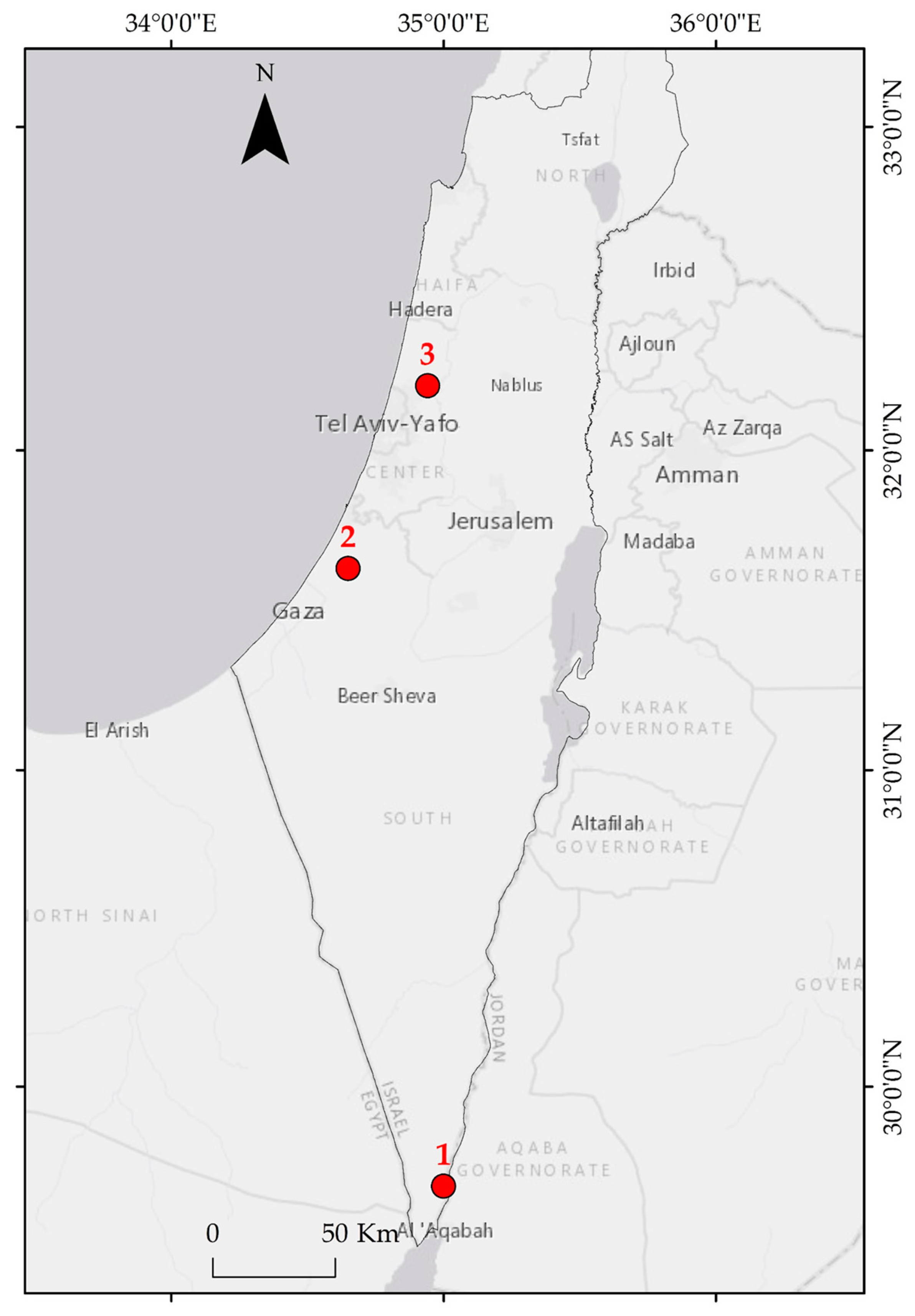
Three different PHC-free types of soil (Table 1) were collected from the surface level (0–5 cm) in Israel (Figure 1). Each type of soil was used to create a dataset of 11 samples with crude oil contamination levels ranging from 0 to 10 wt % with 1 wt % steps (i.e., 0, 1, 2… 10). The crude oil used in this study was composed of heavy n-alkanes (C9H20 and heavier). The preparation of the samples was as follows:
- Each soil type was air-dried and sieved (2 mm).
- For each soil, a mixture of soil and crude oil was created.
- The mixture weighed 1150 g and contained 90 wt % soil and 10 wt % crude oil.
- The mixture was added in increasing amounts to uncontaminated soil samples (weights between 0 and 200 g), thus creating samples of mixture + uncontaminated soil.
- Each sample (mixture + uncontaminated soil) was mixed using a glass stirring stick until a homogeneous sample was obtained.
2.2. Scene Setting and Measurements
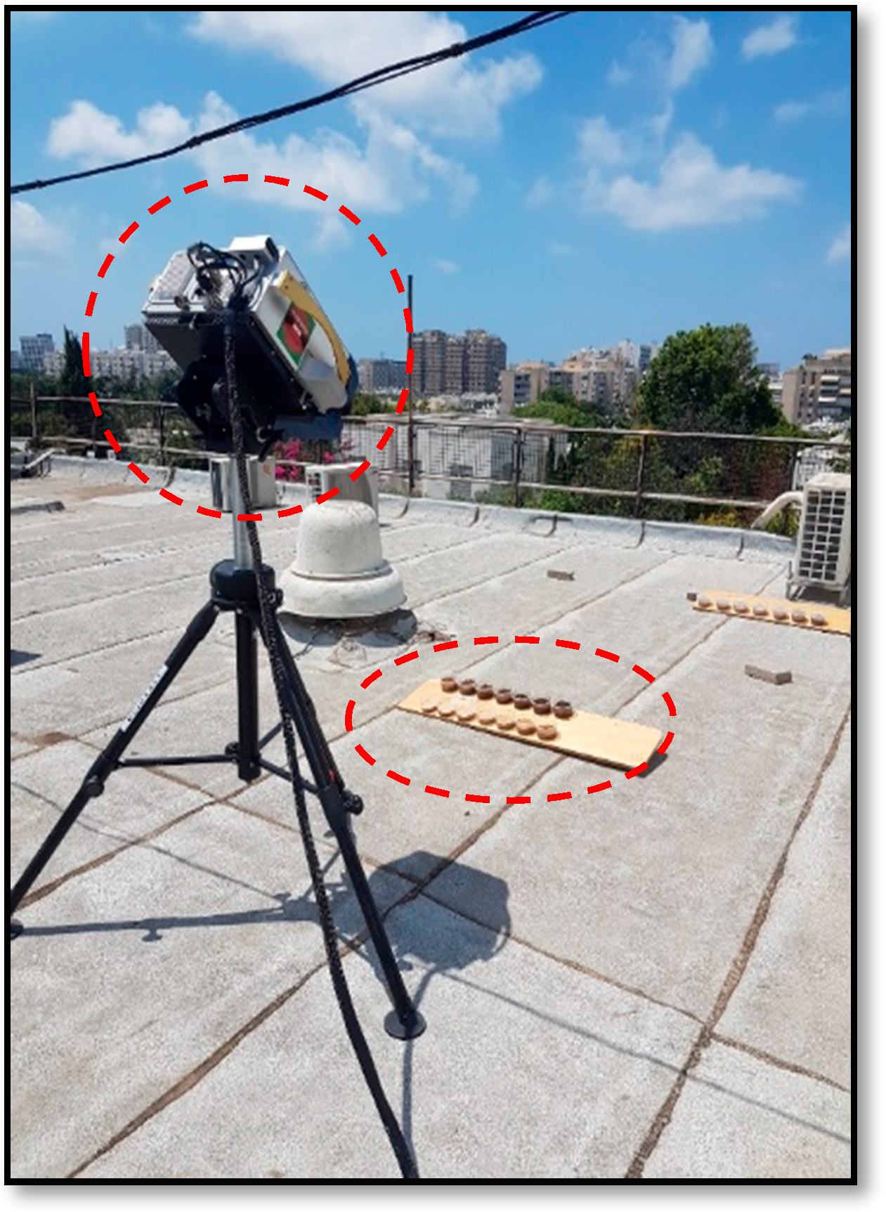
Each sample was evenly distributed on a plastic dish and placed on a wooden panel facing the hyperspectral imaging system geometry (Figure 2).
Each time, samples from a different type of soil were placed on the wooden panel in order to maintain the same distance and geometry for all samples. The measurements took place at noon on 13 August 2018, a warm and sunny day (~30 °C) in Tel Aviv, Israel. For the measurements, a Hyper-Cam LW instrument (Telops, Quebec, Canada) was used, which is a highly advanced HRS sensor that works under the Fourier transform concept and detects the emitted radiation in the LWIR region of the spectrum. It has a spectral resolution of 0.25 cm−1, which provides 88 spectral bands. The incoming infrared radiation from the scene was obtained and recorded by the Hyper-Cam, thus generating an LWIR hyperspectral image. A gold panel plate (Infragold Target, https://www.labsphere.com/labsphere-products-solutions) was also placed in the scene near the samples. The gold panel has low emissivity values throughout the LWIR spectral region and by that it simulates the downwelling radiance from the sky.
2.3. Emissivity Calculations
A Planck fit was generated over the radiance spectrum of all pixels in the samples. That is to say, for each pixel, a blackbody radiation curve was fitted. The measured radiance, for each pixel, can be considered as
where Ls,i is the recorded radiance spectrum of pixel i, is the emissivity of pixel i, Lbb,i is the Planck fit of a pixel i, is the atmosphere attenuation factor, Ld is the sky downwelling radiation (extracted from the gold panel), and Lp is the path radiance to the sensor.
Since the samples were measured from a close distance (a few meters) from the sensor, it can be assumed that , , and thus the emissivity per pixel can be calculated using
2.4. Preprocessing the Data
After the emissivity spectra were calculated for each pixel, a Savitzky–Golay filter was applied to slightly smoothen the spectra. A region of interest for each sample was drawn, and the spectra for the corresponding pixels (~200 pixels per sample) were extracted. Then, a continuum removal (CR) algorithm [23] was applied only on the spectral range of 8–10.5 μm, since in longer wavelengths (10.5 up to 11.2 μm) the spectrum of the soils used in this study is essentially featureless. Thus, a database was established for each type of soil—Hamra, Evrona, and Kokhav.
2.5. Data Analysis
Once the database was established, the analysis of exploring the effect of PHC on the soils, in the LWIR region, was executed. The three predominant spectral absorption features were examined. Firstly, the wavelength of the minimum absorption depth (i.e., the minimum value of the CR spectrum) for each of the predominant spectral features was examined. This was done to understand if increasing PHC contamination causes a shift in absorption features (i.e., change along the x-axis), which might serve as an indicator of PHC presence. Secondly, the CR value of each absorption minimum wavelength was examined to determine whether the level of PHC affects the minimum depth of the spectral feature (i.e., change along the y-axis). Thirdly, partial least square (PLS) regression [24] models were generated: one for all soils together (i.e., generic model) and one per soil type. For each PLS model in this study, 75% of the data were allocated to the model training, and the prediction was made on the remaining 25%. The PLS latent variables (LVs) were selected according to the root-mean-square-error (RMSE) resulting from a stratified k-fold cross-calibration, which preserves the percentage of the pixels for each PHC level and ensures that no sample appears in both datasets (i.e., training and testing). Four evaluation metrics were chosen to evaluate the model’s performance, namely the R2, the slope of the regression line, the RMSE, and the normalized RMSE (nRMSE), which is the ratio between the RMSE and the range of the PHC values (PHCmax − PHCmin). The nRMSE essentially provides the model error in percentage values, which is easier to interpret than RMSE.
The variable importance in the projection (VIP) scores [24] was also calculated. The VIP is a score per predictor (i.e., per spectral band) that essentially tells us what parts of the spectrum are important to predict the response (i.e., PHC level). As a rule of thumb, predictors with a VIP score greater than one are highly relevant to predict the response [25,26].
As mentioned, each pixel was originated from a sample, with a discrete PHC level sample (i.e., 0, 1, 2, …, 10), which was prepared at the lab and labeled accordingly. However, in real life situations, the PHC levels of given samples are continuous rather than discrete. Therefore, in order to simulate a more realistic scenario, and to see how sensitive the PLS model is to noise in the data, two approaches featuring additive noise were taken. In the first approach, a random number from a normal distribution between −1 and 1 was added to the label of the PHC level for all pixels. For example, a pixel with a PHC label of 2 (i.e., a pixel from the 2 PHC wt % sample) was labeled as 2 + a random number, e.g., 2 + 0.32 = 2.32 wt %. This was done for all pixels, in order to create a continuous dataset and to add a certain level of noise. Again, the PLS model was trained on 75% of the data (data + noise), and the prediction was made on 25% (data + noise). This simulates a scenario where the model is trained and the prediction is made upon real samples from the field, which in real life will contain continuous PHC levels. In the second approach, the model was trained on 75% of the original data (a discrete PHC level from lab samples), and the prediction was made on 25% of the data with the added noise. This simulates a scenario where the calibration is made in controlled lab conditions (discrete PHC levels) and the prediction is made on samples from the field (continuous PHC levels). In both approaches, if the PHC level of a pixel resulted in a negative number due to the added random number, the PHC level was set to zero. All of the data pre-processing and analysis was carried out using ENVI software, version 5.2 (Exelis Visual Information Solutions, Boulder, CO, USA), and ad-hoc python scripts, mainly utilizing the scikit-learn library for machine learning [27].
3. Results and Discussion
3.1. Potential Shift in the Spectral Features of the Predominant Minerals
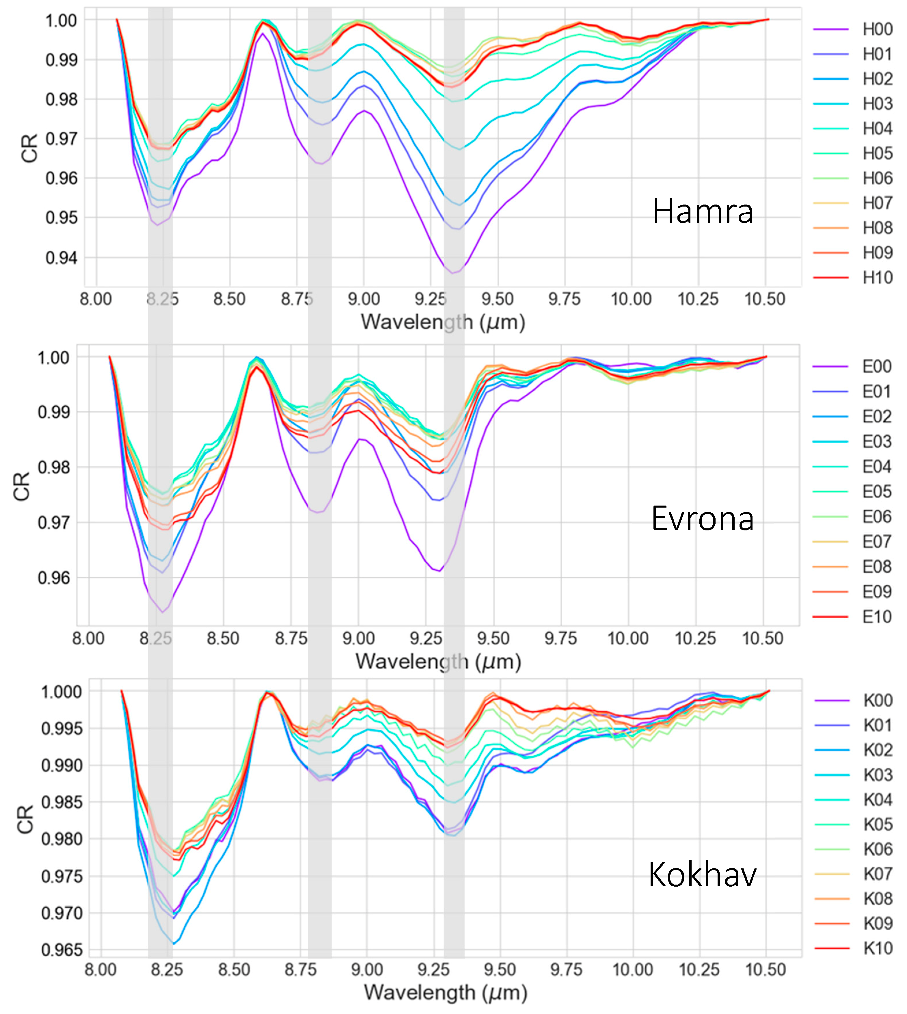
The average CR spectrum, per sample, was plotted for each type of soil to visually observe how the spectrum changes by increasing levels of PHC. All of the soil’s spectra were characterized by three main spectral absorptions at ~8.2, ~8.8, and ~9.2 μm (hereafter Ab_8.2, Ab_8.8, and Ab_9.2) indicating the presence of quartz and clay minerals (The Arizona State University Spectral Library, http://speclib.asu.edu) (Figure 3). It was also observed in the average spectrum that the distinction between low quantities of PHC was visually clearer than for relatively high quantities. It seems that, from a certain amount of PHC contamination (depends on the soil type), the spectrum became saturated and the trend of the spectrum, observed in low quantities, ceased. It is interesting to note that, for the Kokhav soil, the distinction between low quantities was, relatively, not very clear.
Next, the potential shift in the minimum absorption wavelength due to PHC contamination was examined. Figure 4 shows heat maps, per spectral absorption, per soil. For each absorption as well as for each soil, the band that held the minimum absorption depth (i.e., the lowest CR value) was noted per PHC level, per pixel. The percentage of these bands holding the minimum value of specific absorption is shown. In other words, Figure 4 shows the percentage of pixels, per sample, that have a minimum CR value in a specific band. As can be seen, for Ab_8.2 and Ab_9.2, minimum bands are steady and span over 2–3 adjacent spectral bands for all soil types. This situation is somewhat different, as a slight shift, towards shorter wavelengths, was observed for Ab_8.8 in the Hamra and Kokhav soils, whereas no such shift was visible in the Evrona soil, which exhibited a wide range of minimum bands for that absorption. In both soils, Hamra and Kokhav, the shift occurred in the sample with 4 wt % PHC, which might be a threshold that divides the dataset into low and high PHC levels that can be detected using an HRS image in the LWIR spectral region. This is somewhat compatible with the trend visually presented in Figure 3, where the clear difference in spectrum becomes vague due to increasing PHC levels.
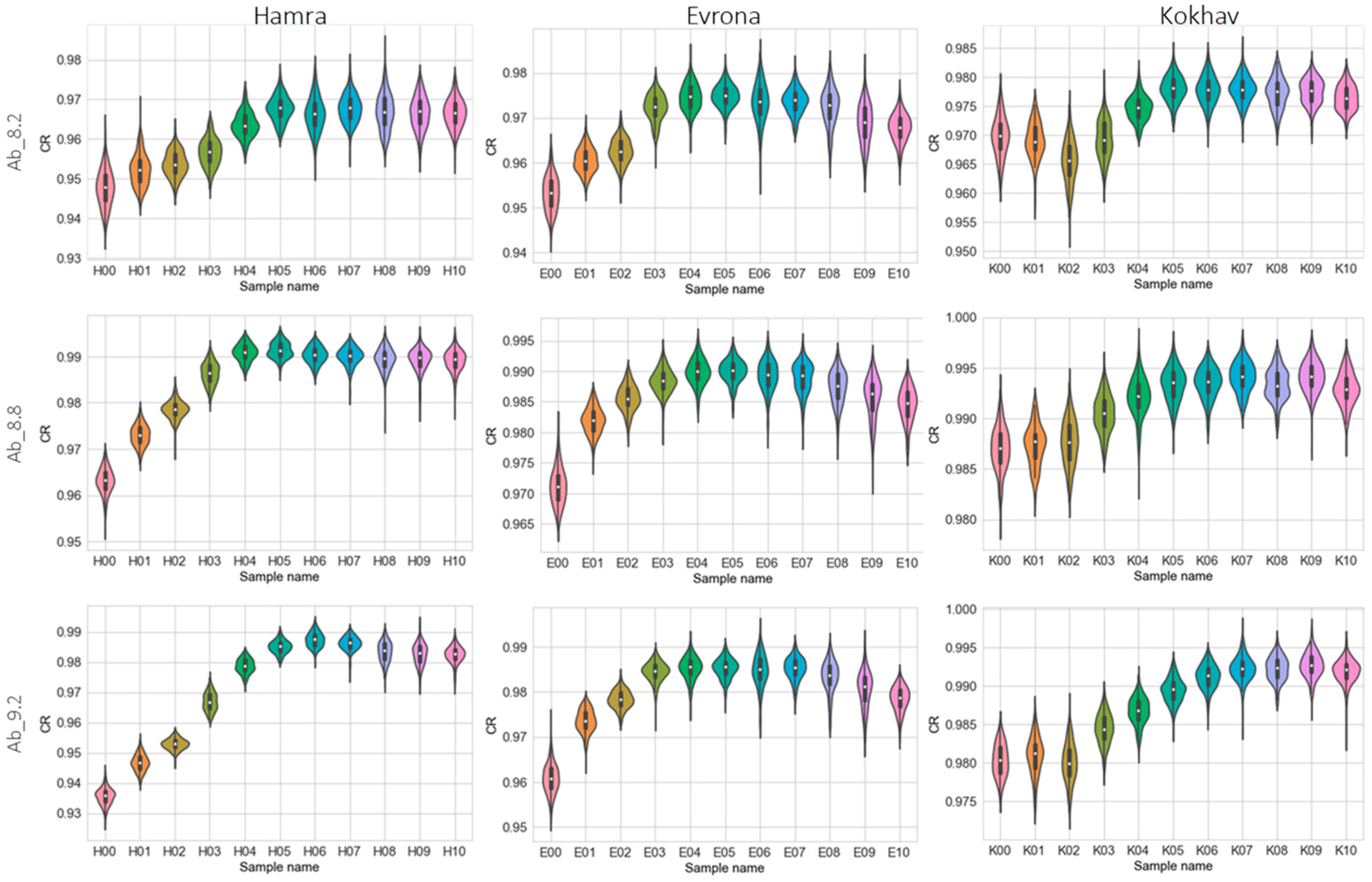
The CR value for each of the minimum wavelengths (from Figure 4), per sample as well as per spectral absorption, is shown in Figure 5 as a violin plot. This kind of plot combines a boxplot and a histogram together, as it shows the range, quantiles, and median of the data as well as the underlying distribution. A similar trend to the one displayed in Figure 3 and Figure 4 is also detectable in Figure 5, where the depth of the spectral features becomes shallower (higher values of CR) as the PHC level increases. When the PHC level reaches ~4 wt %, an increase in the PHC level will not change the depth of the absorption (i.e., the CR value). Moreover, in some cases, the absorption depth is even decreasing with increasing PHC levels, and the CR values resemble the smaller PHC levels such as those in Ab_8.2 and Ab_8.8 in the Evrona soil and in Ab_9.2 in both the Hamra and Evrona soils.
These findings indicate that the PHC does influence the soil spectrum, which is reflected in masking the predominant spectral features, meaning that these spectral absorption features became shallower as a result of an increasing PHC level. However, this trend weakens when the PHC levels reach >4–5 wt %, up to a point where it seems to stop. Saturation occurred, as higher PHC levels did not affect the spectrum. Therefore, the spectral shift of the mineral alone (either along the x-axis or the y-axis), caused by PHC, does not seem to be a good predictor of the PHC level in samples.
3.2. PLS Models
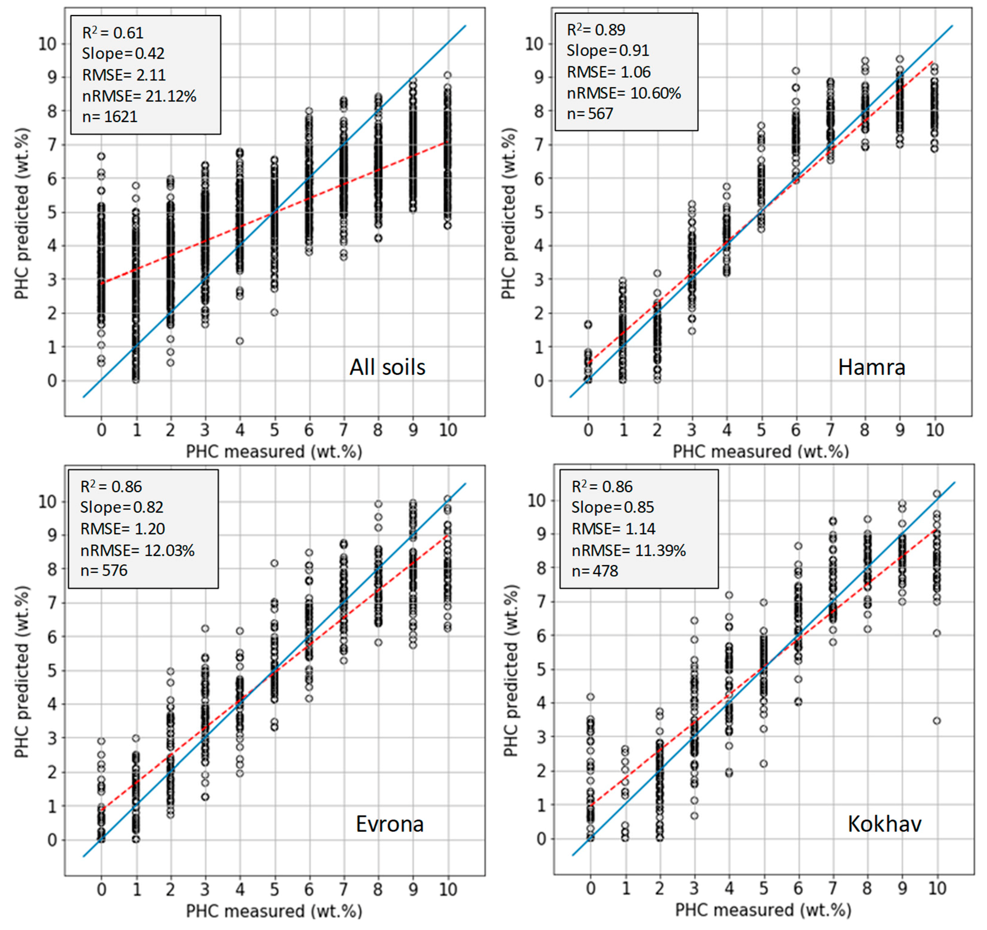
PLS regression models were generated for all soils together (hereafter, the generic model) and per soil type. The PLS model was trained on 75% of the data, and the testing was made on the remaining 25%. As mentioned earlier, the division of 75 and 25% was done using the sklearn library k-fold stratified method, which preserves the percentage of pixels for each PHC level. Figure 6 shows the evaluation metrics of the models.
As can be seen, a major improvement occurs in the evaluation metrics when each soil type has a separate model as opposed to the generic model, which includes the data of all soils combined. For example, the R2 improved from 0.61 in the generic model to >0.85 in each type of soil, and the RMSE was almost double in the generic mode (2.11 wt %) than in the other PLS models (~1.1 wt %). From this result, we can deduce that a generic model is inferior to the other models, and in practice an individual model per soil type is recommended. When examining the differences between the soils, the Hamra soil had the best evaluation metrics, e.g., a slope of 0.91 and an nRMSE = 10.6%. Evrona and Kokhav display similar results (e.g., R2 = 0.86) with a small advantage to Kokhav, e.g., RMSE = 1.14 wt % in comparison to RMSE = 1.20 wt %.
In addition, the trend shown in the previous figures (ascending trend up to ~4–5 wt % and then saturation) extends up to a PHC level of about 7–8 wt %. That is to say, there is a clear trend and a good fit between measured and predicted values, up to a higher PHC level. From that PHC level onward, the trend is mitigated. This is especially clear in the Hamra soil and less obvious in the Evrona and Kokhav soil. Since the trend was mitigated towards higher PHC levels, it was intriguing to calculate the evaluation metrics for each range of samples starting from *00-*05 (where * denotes the soil type) and adding one more sample each time. Table 2 summarizes the results of this notion. Interesting behavior can be deduced. In general, the model metrics are improving when not all the PHC levels are accounted for. The R2, slope, and nRMSE of Evrona are at their peak values in the first range of the sample (i.e., from E00 to E05), whereas for Hamra and Kokhav the peaks occur in the second and third range of the sample. For example, in the Hamra soil, the nRMSE is almost half (5.82%) when considering the PHC level of 0–6 wt % in comparison to the nRMSE in 0–10 wt % PHC levels (10.6%), and the R2 increases from 0.89 to 0.97. Even though the original model for Hamra (H00-H10) shows good results, this is a major improvement. This kind of improvement is less pronounced in Evrona, where the R2, slope, and nRMSE are relatively constant throughout all ranges. As opposed to that, the Kokhav soil shows that the model improves when more PHC is added. The worst evaluation metrics, with nRMSE = 14.87%, are found when the PHC levels are 0–5 wt %, and the nRMSE decreases to 11.39% when all samples are accounted for. This is reflected in the coefficient of variance (CV) shown in Table 2, as the CV of Evrona’s nRMSE is 8.69%, and the CVs of the nRMSE of Hamra and Kokhav are much higher. These results imply that not only is a specific model per soil superior to a generic model, but also that each soil might have an optimum threshold of PHC to generate the PLS model.
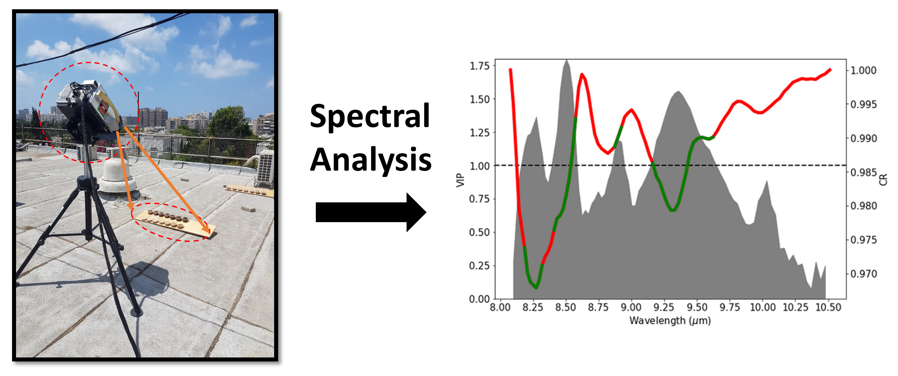
3.3. Variable Importance in Projection (VIP)
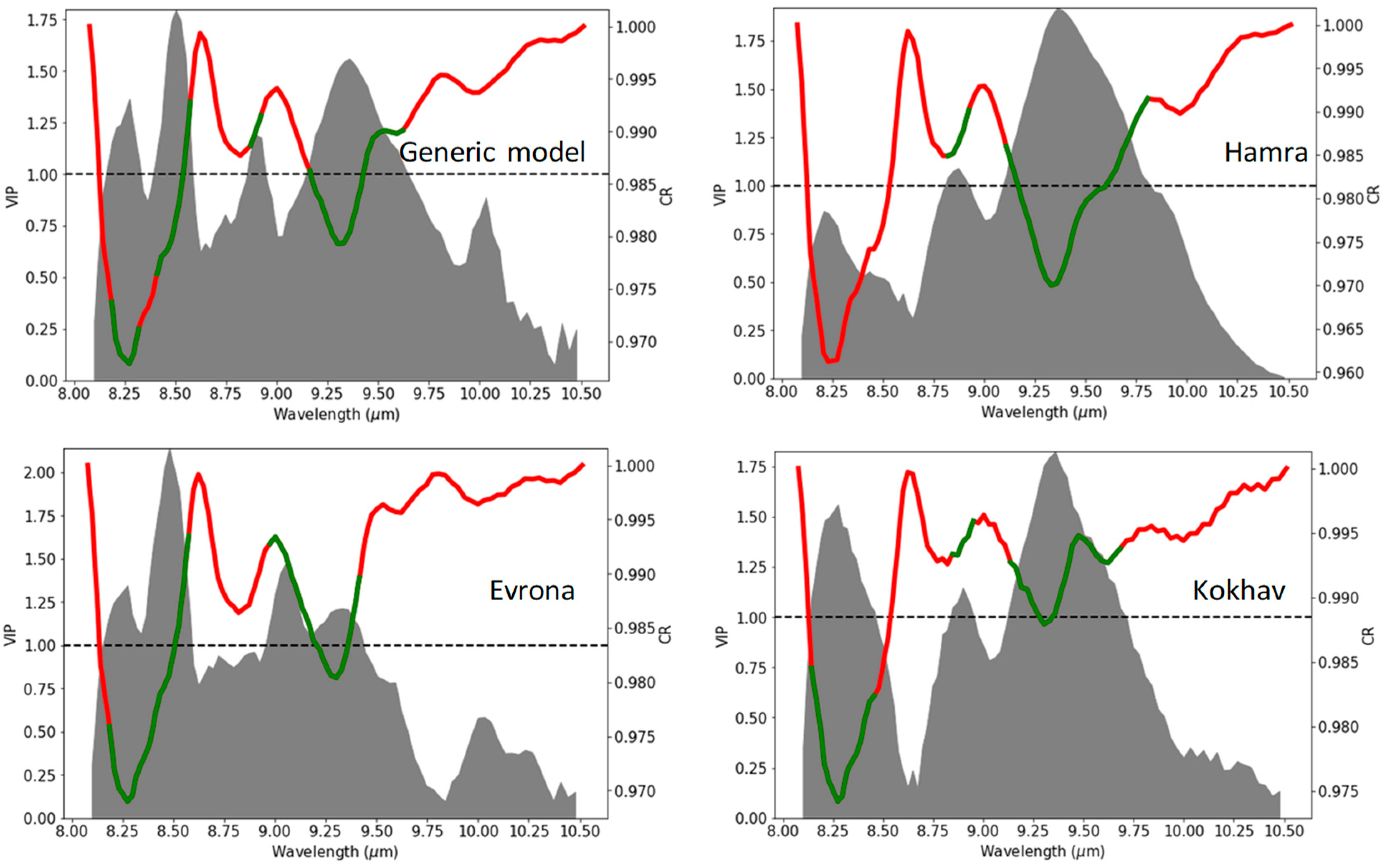
VIP scores were calculated for the generic model and for each individual soil model (Figure 7). VIP scores reveal the most important and most influential bands within the prediction model. Generally, the areas with high VIP scores (green sections of the average spectrum) are located in the spectral absorption features, namely Ab_8.2, AB_8.8, and Ab_9.2. These findings clearly highlight the effect of PHC on the spectrum and indicate that PHC has some spectral alteration effects on the predominant minerals of the different soils. In addition, the ~9.5 μm band (and its neighbors), which received a relativity high VIP score in all models, was also found to be a good indicator for the detection of PHC in soils by [15].
When zooming in to examine the differences between the models, one can notice that only the Ab_9.2 is constant throughout all models. For example, the Ab_8.2 received high values in both Evrona and Kokhav but was omitted from Hamra. A similar case can be seen in Ab_8.8. Its right-hand section appears important in Hamra and Kokhav, but is excluded from Evrona’s high VIP spectral regions. Moreover, even when the same spectral feature received high VIP scores in different models, its influence might be different. For example, in Hamra and Kokhav, Ab_9.2 seems to have the most important spectral regions, with the highest VIP scores, whereas in Evrona the same spectral feature seems to be of secondary importance due to lower VIP values in comparison to Ab_8.2.
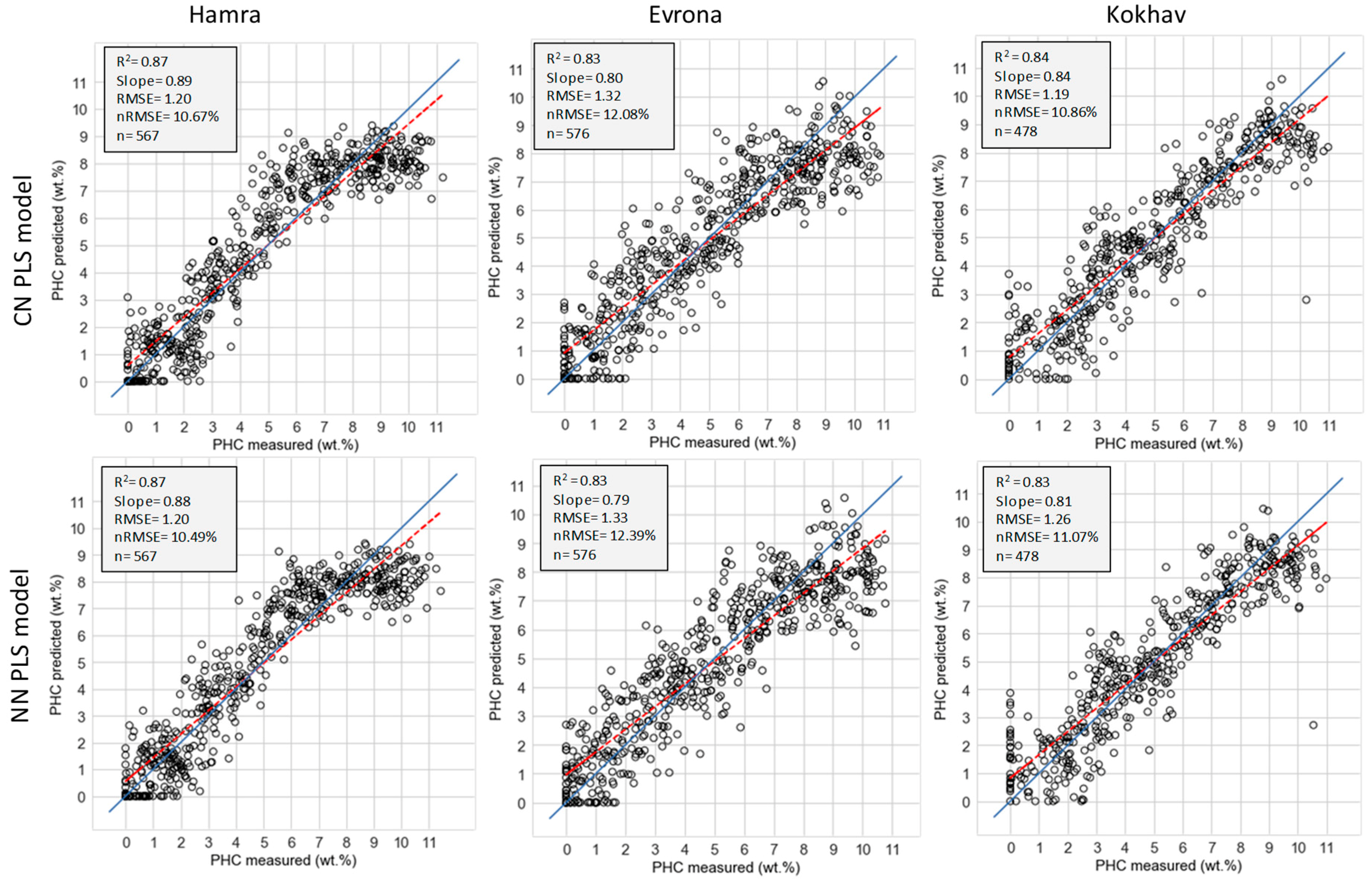
3.4. PLS Models with Additive Noise
Since the database consisted of pixels coming from discrete PHC levels (i.e., 0, 1, 2, etc.), some noise was added to the PHC label of each pixel in order to obtain continuous PHC values, which simulates a more realistic scenario. As mentioned earlier, two approaches were taken only for the PLS models per individual soil. In the first approach, a random number between −1 and 1, from a normal distribution, was added to each pixel PHC label and the PLS model was then executed. Since this PLS model was trained and tested on the data with added noise, it will henceforth be referred to as NN (noise–noise). In the second approach, the noise was only added to 25% of the testing data, and because of that it will henceforth be referred to as CN (clean–noise). Again, pixels that ended up with a negative value of PHC level were set to zero. These PLS models and evaluation metrics were calculated, and the results are shown in Figure 8.
No major difference is observed between the NN and CN PLS models across all soils. For example, the R2 of Hamra and Evrona did not change, and in Kokhav it slightly decreased from 0.84 (CN) to 0.83 (NN). The slope, RMSE, and nRMSE display a negligible change in all soils.
Table 3 compares all (per soil) PLS models generated in this study. The PLS models in Figure 6 are referred to as CC (clean–clean) in Table 3, as they were trained and tested on clean data without additive noise. As can be seen in the summarized results, the differences in the evaluation metrics within each type of soil are minor. For example, the R2 in Hamra was 0.89, 0.87, and 0.87, the nRMSE in Evrona was 12.03, 12.39, and 12.08%, and the slope for Kokhav was 0.85, 0.81, and 0.84 for the CC, NN, and CN models, respectively. It can be concluded that the models developed in this study and the resulting predictions are robust and stable.
Table 3 also shows that the difference between the soils regarding the ability to predict the PHC level based on their LWIR spectrum are not drastic, even though they have different characteristics (Table 1). Nevertheless, it seems that the Hamra soil is the most favorable to PHC detection using the method utilized in this study, followed by Kokhav and Evrona. This might be the attribute to the grain size as Hamra has a coarser grain size than Evrona and Kokhav. A soil with a coarser grain size (Hamra) absorbs more light (a good absorber) than soil with fine particles (Kokhav) [28,29,30], which might result in a more intense radiance emission (a good emitter) of the soil with a coarser grain size (Hamra) and thus a stronger signal. Another factor that should be taken into consideration is that the crude oil has a more specific surface area in finer particles and thus spreads over a larger area, which might cause the crude oil effect to be less dominant in the emitted radiance.
The implementation of these results can be drawn into practice by considering the type of soil one would like to examine using HRS imagery in the LWIR spectral region. In addition, the potential of existing and future LWIR sensors to detect and quantify PHC in soils can be evaluated by the location of the spectral bands, as this study showed that specific spectral regions are more important to the PHC prediction than others.
4. Conclusions
This study explored the effect of PHC (originated from crude oil) on the LWIR spectrum of three different soil types. To that end, the spectra of 11 lab-prepared samples, per soil type, were recorded using a Telops HyperCam LWIR imaging system in an outdoor condition. As PHC does not have fundamental vibrations in the LWIR spectral region, this study monitored the spectral changes of the minerals found in these soils due to the PHC effect. No meaningful shift in the spectral absorption of the minerals, both in the location and in the depth, was found with increasing amounts of PHC. A generic PLS model (a model with all soils) was found inferior to the models per soil type. The VIP results showed important spectral regions for the predictions of PHC, which were in the spectral range of the predominant minerals. However, not all soils had the same importance for the same spectral features. Three PLS models (one with the original data and two with additive noise) were utilized to explore the possibility of predicting the PHC level in each type of soil from the calculated emissivity. All PLS models showed good evaluation metrics: an R2 of 0.83–0.89, a slope of 0.79–0.91, an RMSE of 1.06–1.33 wt %, and an nRMSE of 10.42–12.39%. These results might be considered as a proof of concept that PHC can be detected with good accuracy in soils from LWIR hyperspectral images. Implication for future remote sensing platforms that use LWIR hyperspectral imagery instruments can be drawn from this study. Moreover, as this experiment has been executed under outdoor conditions with a sensor that is meant to fly onboard an actual airplane, the method and results presented here might be adapted to an image from a real scenario acquired from the air domain.
Author Contributions
Conceptualization, R.P. and E.B.-D.; formal analysis, methodology, investigation, visualization, and original draft preparation, R.P.; resources, supervision, and review & editing, E.B.-D.
Funding
This research received no external funding.
Acknowledgments
The authors would like to thank the members of the remote sensing laboratory at Tel Aviv University for their constructive comments and specifically to Shahar Weksler for operating the Hyper-Cam instrument and producing the raw images. We also appreciated the crude oil provided by Arnon Karnieli from Ben-Gurion University.
Conflicts of Interest
The authors declare no conflict of interest.
References
- Ramirez, M.I.; Arevalo, A.P.; Sotomayor, S.; Bailon-Moscoso, N. Contamination by oil crude extraction—Refinement and their effects on human health. Environ. Pollut. 2017, 231, 415–425. [Google Scholar] [CrossRef] [PubMed]
- Aguilera, F.; Méndez, J.; Pásaro, E.; Laffon, B. Review on the effects of exposure to spilled oils on human health. J. Appl. Toxicol. JAT 2010, 30, 291–301. [Google Scholar] [CrossRef] [PubMed]
- Chima, U.D.; Vure, G. Implications of crude oil pollution on natural regeneration of plant species in an oil-producing community in the Niger Delta Region of Nigeria. J. For. Res. 2014, 25, 915–921. [Google Scholar] [CrossRef]
- Shapiro, K.; Khanna, S.; Ustin, S.; Shapiro, K.; Khanna, S.; Ustin, S.L. Vegetation Impact and Recovery from Oil-Induced Stress on Three Ecologically Distinct Wetland Sites in the Gulf of Mexico. J. Mar. Sci. Eng. 2016, 4, 33. [Google Scholar] [CrossRef]
- Cloutis, E.A. Spectral reflectance properties of hydrocarbons: Remote-sensing implications. Science 1989, 245, 165–168. [Google Scholar] [CrossRef] [PubMed]
- Stuart, B.H. Infrared Spectroscopy: Fundamentals and Applications, 1st ed.; Wiley: Chichester, UK; Hoboken, NJ, USA, 2004; ISBN 978-0-470-85428-0. [Google Scholar]
- Schwartz, G.; Ben-Dor, E.; Eshel, G. Quantitative Analysis of Total Petroleum Hydrocarbons in Soils: Comparison between Reflectance Spectroscopy and Solvent Extraction by 3 Certified Laboratories. Appl. Environ. Soil Sci. 2012, 2012, e751956. [Google Scholar] [CrossRef]
- Winkelmann, K.H. On the Applicability of Imaging Spectrometry for the Detection and Investigation of Contaminated Sites with Particular Consideration Given to the Detection of Fuel Hydrocarbon Contaminants in Soil. Ph.D. Thesis, Brandenburg University of Technology, Senftenberg, Germany, 2005. [Google Scholar]
- Hörig, B.; Kühn, F.; Oschütz, F.; Lehmann, F. HyMap hyperspectral remote sensing to detect hydrocarbons. Int. J. Remote Sens. 2001, 22, 1413–1422. [Google Scholar] [CrossRef]
- Scafutto, R.D.M.; de Filho, C.R.S.; de Oliveira, W.J. Hyperspectral remote sensing detection of petroleum hydrocarbons in mixtures with mineral substrates: Implications for onshore exploration and monitoring. ISPRS J. Photogramm. Remote Sens. 2017, 128, 146–157. [Google Scholar] [CrossRef]
- Kruse, F.A. Imaging SpectrometryUse of airborne imaging spectrometer data to map minerals associated with hydrothermally altered rocks in the northern grapevine mountains, Nevada, and California. Remote Sens. Environ. 1988, 24, 31–51. [Google Scholar] [CrossRef]
- Forrester, S.T.; Janik, L.J.; McLaughlin, M.J.; Soriano-Disla, J.M.; Stewart, R.; Dearman, B. Total Petroleum Hydrocarbon Concentration Prediction in Soils Using Diffuse Reflectance Infrared Spectroscopy. Soil Sci. Soc. Am. J. 2013, 77, 450–460. [Google Scholar] [CrossRef]
- Hazel, G.; Bucholtz, F.; Aggarwal, I.D.; Nau, G.; Ewing, K.J. Multivariate Analysis of Mid-IR FT-IR Spectra of Hydrocarbon-Contaminated Wet Soils. Appl. Spectrosc. 1997, 51, 984–989. [Google Scholar] [CrossRef]
- Molpeceres, G.; Timón, V.; Jiménez-Redondo, M.; Escribano, R.; Maté, B.; Tanarro, I.; Herrero, V.J. Structure and infrared spectra of hydrocarbon interstellar dust analogs. Phys. Chem. Chem. Phys. 2017, 19, 1352–1360. [Google Scholar] [CrossRef] [PubMed] [Green Version]
- Van der Meijde, M.; Knox, N.M.; Cundill, S.L.; Noomen, M.F.; van der Werff, H.M.A.; Hecker, C. Detection of hydrocarbons in clay soils: A laboratory experiment using spectroscopy in the mid- and thermal infrared. Int. J. Appl. Earth Obs. Geoinf. 2013, 23, 384–388. [Google Scholar] [CrossRef]
- Pelta, R.; Ben-Dor, E. Assessing the detection limit of petroleum hydrocarbon in soils using hyperspectral remote-sensing. Remote Sens. Environ. 2019, 224, 145–153. [Google Scholar] [CrossRef]
- Schumacher, D. Hydrocarbon-Induced Alteration of Soils and Sediments. AAPG Memoir 1996, 71–89. [Google Scholar] [CrossRef]
- Agassi, E.; Hirsch, E.; Ronen, A. Spectral and spatial measurements of atmospheric aerosol clouds with a hyperspectral sensor. In SPIE Proceedings, Electro-Optical Remote Sensing, Photonic Technologies, and Applications IV; Kamerman, G.W., Steinvall, O., Lewis, K.L., Hollins, R.C., Merlet, T.J., Bishop, G.J., Gonglewski, J.D., Eds.; SPIE: Bellingham, WA, USA, 2010; p. 78350I. [Google Scholar]
- Eisele, A.; Chabrillat, S.; Hecker, C.; Hewson, R.; Lau, I.C.; Rogass, C.; Segl, K.; Cudahy, T.J.; Udelhoven, T.; Hostert, P.; et al. Advantages using the thermal infrared (TIR) to detect and quantify semi-arid soil properties. Remote Sens. Environ. 2015, 163, 296–311. [Google Scholar] [CrossRef]
- McDowell, M.L.; Kruse, F.A. Integrated visible to near infrared, short wave infrared, and long wave infrared spectral analysis for surface composition mapping near Mountain Pass, California. In SPIE Proceedings; SPIE: Bellingham, WA, USA, 2015; Volume 9472, p. 94721C. [Google Scholar]
- Notesco, G.; Kopačková, V.; Rojík, P.; Schwartz, G.; Livne, I.; Dor, E.B. Mineral Classification of Land Surface Using Multispectral LWIR and Hyperspectral SWIR Remote-Sensing Data. A Case Study over the Sokolov Lignite Open-Pit Mines, the Czech Republic. Remote Sens. 2014, 6, 7005–7025. [Google Scholar] [CrossRef] [Green Version]
- Vaughan, R.G.; Calvin, W.M.; Taranik, J.V. SEBASS hyperspectral thermal infrared data: surface emissivity measurement and mineral mapping. Remote Sens. Environ. 2003, 85, 48–63. [Google Scholar] [CrossRef]
- Clark, R.N.; Roush, T.L. Reflectance spectroscopy: Quantitative analysis techniques for remote sensing applications. J. Geophys. Res. 1984, 89, 12. [Google Scholar] [CrossRef]
- Wold, S.; Sjöström, M.; Eriksson, L. PLS-regression: A basic tool of chemometrics. Chemom. Intell. Lab. Syst. 2001, 58, 109–130. [Google Scholar] [CrossRef]
- Tran, T.N.; Afanador, N.L.; Buydens, L.M.C.; Blanchet, L. Interpretation of variable importance in Partial Least Squares with Significance Multivariate Correlation (sMC). Chemom. Intell. Lab. Syst. 2014, 138, 153–160. [Google Scholar] [CrossRef]
- Chong, I.-G.; Jun, C.-H. Performance of some variable selection methods when multicollinearity is present. Chemom. Intell. Lab. Syst. 2005, 78, 103–112. [Google Scholar] [CrossRef]
- Pedregosa, F.; Varoquaux, G.; Gramfort, A.; Michel, V.; Thirion, B.; Grisel, O.; Blondel, M.; Prettenhofer, P.; Weiss, R.; Dubourg, V.; et al. Scikit-learn: Machine Learning in Python. J. Mach. Learn. Res. 2011, 12, 2825–2830. [Google Scholar]
- Sadeghi, M.; Babaeian, E.; Tuller, M.; Jones, S. Particle size effects on soil reflectance explained by an analytical radiative transfer model. Remote Sens. Environ. 2018, 210, 375–386. [Google Scholar] [CrossRef]
- Bogrekci, I.; Lee, W.S. Improving phosphorus sensing by eliminating soil particle size effect in spectral measurement. Trans. ASAE 2005, 48, 1971–1978. [Google Scholar] [CrossRef]
- Udvardi, B.; Kovács, I.J.; Fancsik, T.; Kónya, P.; Bátori, M.; Stercel, F.; Falus, G.; Szalai, Z. Effects of Particle Size on the Attenuated Total Reflection Spectrum of Minerals. Appl. Spectrosc. 2017, 71, 1157–1168. [Google Scholar] [CrossRef] [PubMed]
Figure 1.
The location from which the soil types were collected: Evrona, Kokhav Michael, and Nir Eliyahu denoted as 1, 2, and 3, respectively.
Figure 1.
The location from which the soil types were collected: Evrona, Kokhav Michael, and Nir Eliyahu denoted as 1, 2, and 3, respectively.

Figure 2.
The setting of the study. The HyperCam-LW and the samples are marked in dashed red circles.
Figure 2.
The setting of the study. The HyperCam-LW and the samples are marked in dashed red circles.

Figure 3.
The average spectrum (average of all pixels), per sample, for the three soils in continuum removal (CR) values. The grey lines indicate three main mineral absorptions (at ~8.2, ~8.8, and ~9.2 μm), which were caused by a mix of quartz and clay minerals. In the legend of each plot, the first letter indicates the soil type (H = Hamra, E = Evrona, and K = Kokhav), and the two digits that follow represent the petroleum hydrocarbon (PHC) level in wt %. Note that a distinguished difference can be observed between samples with relatively low concentration, whereas the differences between relatively high PHC levels are less clear.

Figure 4.
Heat maps showing the percentage of the pixels, per sample, with a minimum CR value at a specific wavelength. Ab_8.2, Ab_8.8, and Ab_9.2 indicate heat maps for the spectral features at 8.2, 8.8, and 9.2 μm, respectively. Note that a slight shift towards shorter wavelengths was observed in Ab_8.8 for the Hamra (H) and Kokhav (K) soils.

Figure 5.
A violin plot, per soil, per dominant spectral feature. Each plot displays the distribution of the minimum CR values of all pixels, per sample. Note that from a PHC level of about 4 wt %, the ascending trend is mitigated and, in some cases, even turns to a descending trend. The different colors of the samples serve visualization purposes.

Figure 6.
Partial least square (PLS) models for a generic model (all soils) and per soil. The dashed red line denotes the regression line and the solid blue line denotes a y = x line. The generic model metrics are moderate, whereas the PLS models per soils show good evaluation metrics. Note that from a certain PHC level (~7–8 wt %), the models have difficulties in making a good estimation. This is most pronounced in Hamra.

Figure 7.
VIP scores per PLS model (grey area) with an average spectrum for reference (red-green curve) are shown. The red parts of the average spectrum are bands with VIP <1 and the green sections are bands with VIP >1. The black dashed line represents VIP = 1. Note that not all spectral features (i.e., spectral absorptions) have a high VIP score.

Figure 8.
Two PLS models with added noise to each pixel create a more realistic scenario. The dashed red line denotes the regression line and the solid blue line denotes a y = x line. NN means that the model was trained and tested on data with added noise, and CN means that the noise was added only to the testing dataset. Good evaluation metrics are found across all soil types despite the added noise and the differences between the soils.


Table 1.
The types of soil used in this study. The code column represents the names of soils used in the text.
Table 1.
The types of soil used in this study. The code column represents the names of soils used in the text.
| Code | Local Name | USDA | Location | Description | PSD (% volume) | Texture | ||
|---|---|---|---|---|---|---|---|---|
| Clay (<2 μm) | Silt (2 to 50 μm) | Sand (>50 μm) | ||||||
| Evrona | Salt playa | Salorthids | Evrona playa (Beer Ora), Israel | Evrona playa is a salt flat, consists of CaCO3 and other salts. | 3.8 | 21.0 | 75.2 | Loamy sand |
| Hamra | Red sand soil | Rhodoxeralfs | Kibbutz Nir -Eliyahu, Israel | Sandy red soil. Its grains are covered by minerals and iron oxide, aluminum oxide and Manganese. | 2.4 | 4.8 | 92.8 | Sand |
| Kokhav | Dark-clay soil | Haploxeralfs | Kibbutz Kokahv Michael, Israel | This soil is located at a transition area and therefore it is a mixture of alluvium soil and grumusol mixed with sand. | 12.4 | 34.4 | 53.2 | Sandy Loam |
Table 2.
The resulted model evaluation metrics for different ranges of samples is shown. The two digits in the sample name denote the PHC level (00 means PHC of 0 wt %; 07 means PHC of 7 wt %). Mean, STD (standard deviation), and CV (coefficient of variance) were also calculated to indicate the variance for each metric. All soils show a similar trend in evaluation metrics, Hamra is improving with less PHC, Evrona is indifferent to PHC levels, and Kokhav is improving with more PHC.
| Samples | n | R2 | Slope | RMSE (wt %) | nRMSE (%) | |
|---|---|---|---|---|---|---|
| Hamra | H00-H05 | 323 | 0.96 | 0.95 | 0.32 | 6.45 |
| H00-H06 | 371 | 0.97 | 0.96 | 0.35 | 5.82 | |
| H00-H07 | 421 | 0.96 | 0.97 | 0.49 | 6.94 | |
| H00-H08 | 460 | 0.94 | 0.96 | 0.66 | 8.19 | |
| H00-H09 | 517 | 0.91 | 0.93 | 0.89 | 9.88 | |
| H00-H10 | 567 | 0.89 | 0.91 | 1.06 | 10.60 | |
| Mean | 0.94 | 0.94 | 0.63 | 7.98 | ||
| STD | 0.03 | 0.02 | 0.27 | 1.76 | ||
| CV | 3.10% | 2.17% | 43.46% | 22.06% | ||
| Evrona | E00-E05 | 320 | 0.92 | 0.91 | 0.47 | 9.47 |
| E00-E06 | 368 | 0.91 | 0.88 | 0.59 | 9.91 | |
| E00-E07 | 421 | 0.90 | 0.86 | 0.72 | 10.25 | |
| E00-E08 | 474 | 0.90 | 0.85 | 0.82 | 10.25 | |
| E00-E09 | 531 | 0.87 | 0.83 | 1.05 | 10.62 | |
| E00-E10 | 567 | 0.86 | 0.82 | 1.20 | 12.03 | |
| Mean | 0.89 | 0.85 | 0.80 | 10.58 | ||
| STD | 0.02 | 0.03 | 0.25 | 0.92 | ||
| CV | 2.38% | 3.52% | 31.21% | 8.69% | ||
| Kokhav | K00-K05 | 267 | 0.79 | 0.81 | 0.74 | 14.87 |
| K00-K06 | 315 | 0.86 | 0.89 | 0.72 | 12.02 | |
| K00-K07 | 355 | 0.89 | 0.91 | 0.73 | 10.44 | |
| K00-K08 | 394 | 0.89 | 0.90 | 0.81 | 10.08 | |
| K00-K09 | 438 | 0.88 | 0.87 | 0.95 | 10.57 | |
| K00-K10 | 478 | 0.86 | 0.85 | >1.14 | 11.39 | |
| Mean | 0.86 | 0.87 | 0.84 | 11.56 | ||
| STD | >0.03 | 0.03 | 0.15 | 1.61 | ||
| CV | 3.98% | 3.88% | 17.94% | 13.95% |
Table 3.
Summary of the evaluation metrics for PLS models. Note that there are practically no differences between the PLS models within each soil. The Hamra soil has the best evaluation metrics amongst the soils, followed by Kokhav and Evrona. Nevertheless, the differences between the soils are not large.
| Soil Type | Model | Figure | R2 | Slope | RMSE (wt %) | nRMSE (%) |
|---|---|---|---|---|---|---|
| Hamra | CC | 5 | 0.89 | 0.91 | 1.06 | 10.60 |
| NN | 7 | 0.87 | 0.88 | 1.20 | 10.49 | |
| CN | 7 | 0.87 | 0.89 | 1.20 | 10.67 | |
| Evrona | CC | 5 | 0.86 | 0.82 | 1.20 | 12.03 |
| NN | 7 | 0.83 | 0.79 | 1.33 | 12.39 | |
| CN | 7 | 0.83 | 0.80 | 1.32 | 12.08 | |
| Kokhav | CC | 5 | 0.86 | 0.85 | 1.14 | 11.39 |
| NN | 7 | 0.83 | 0.81 | 1.26 | 11.07 | |
| CN | 7 | 0.84 | 0.84 | 1.19 | 10.86 |
© 2019 by the authors. Licensee MDPI, Basel, Switzerland. This article is an open access article distributed under the terms and conditions of the Creative Commons Attribution (CC BY) license (http://creativecommons.org/licenses/by/4.0/).
Share and Cite
MDPI and ACS Style
Pelta, R.; Ben-Dor, E. An Exploratory Study on the Effect of Petroleum Hydrocarbon on Soils Using Hyperspectral Longwave Infrared Imagery. Remote Sens. 2019, 11, 569. https://doi.org/10.3390/rs11050569
AMA Style
Pelta R, Ben-Dor E. An Exploratory Study on the Effect of Petroleum Hydrocarbon on Soils Using Hyperspectral Longwave Infrared Imagery. Remote Sensing. 2019; 11(5):569. https://doi.org/10.3390/rs11050569
Chicago/Turabian StylePelta, Ran, and Eyal Ben-Dor. 2019. "An Exploratory Study on the Effect of Petroleum Hydrocarbon on Soils Using Hyperspectral Longwave Infrared Imagery" Remote Sensing 11, no. 5: 569. https://doi.org/10.3390/rs11050569
Note that from the first issue of 2016, this journal uses article numbers instead of page numbers. See further details here.