Assessment of MERRA-2 Surface PM2.5 over the Yangtze River Basin: Ground-based Verification, Spatiotemporal Distribution and Meteorological Dependence


Abstract
:1. Introduction
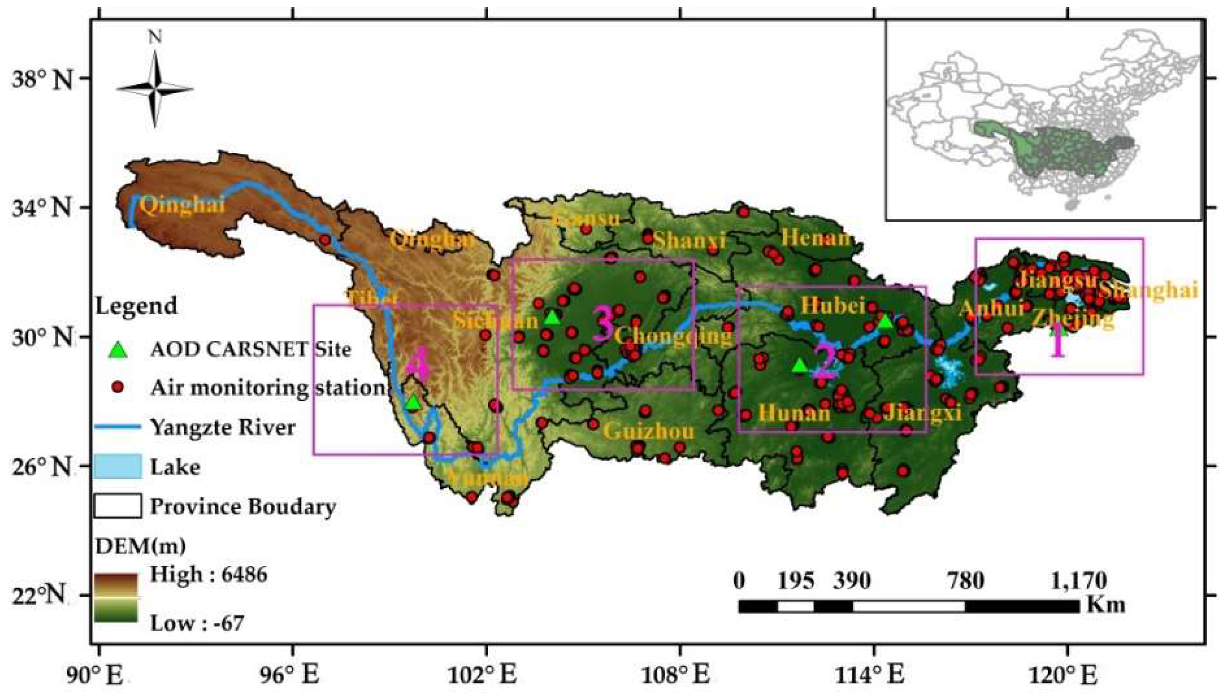
2. Data and Methods
2.1. Data
2.2. Methods
2.2.1. Comparison Analysis
2.2.2. Trend Analysis
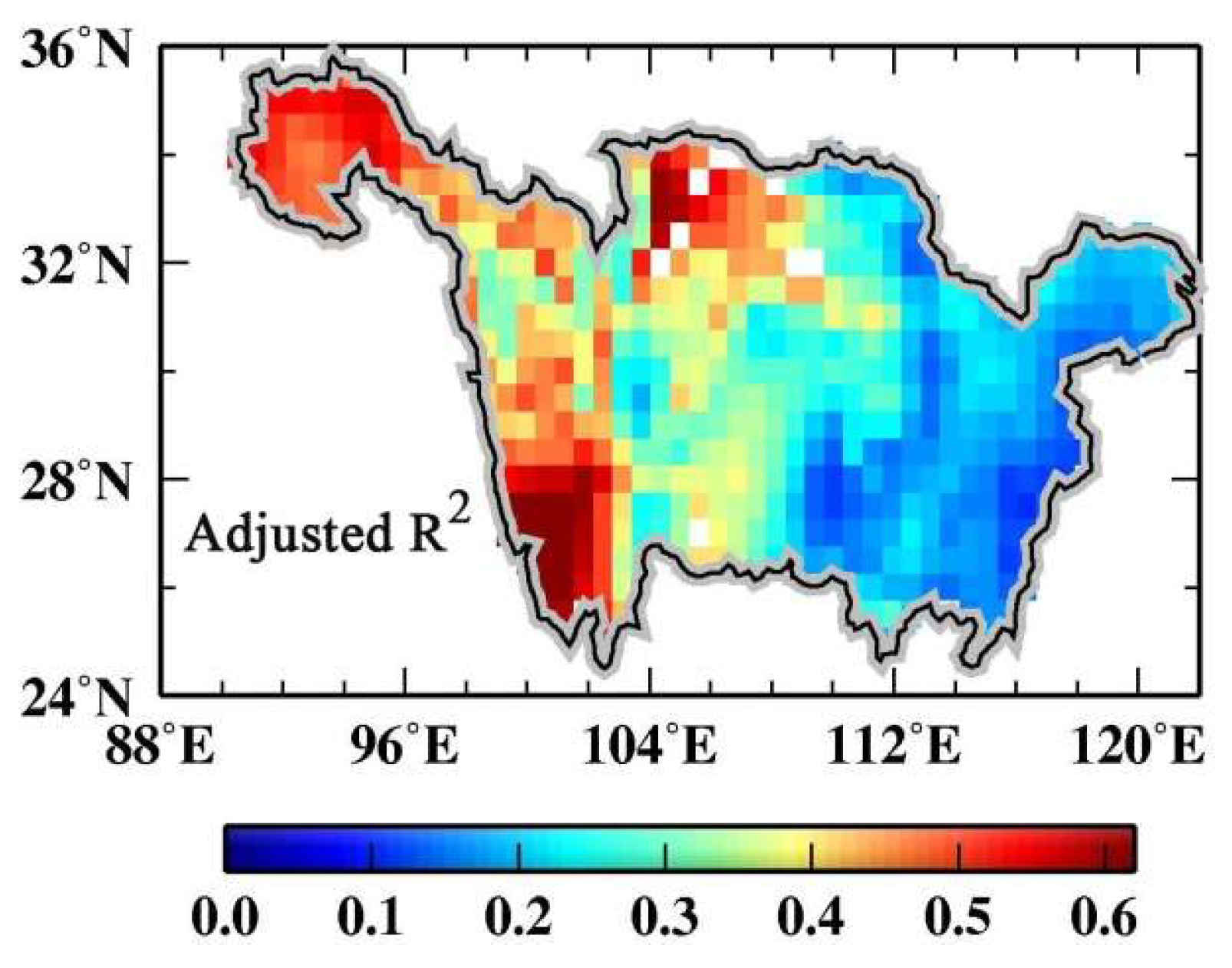
2.2.3. Multiple Linear Regression
3. Results
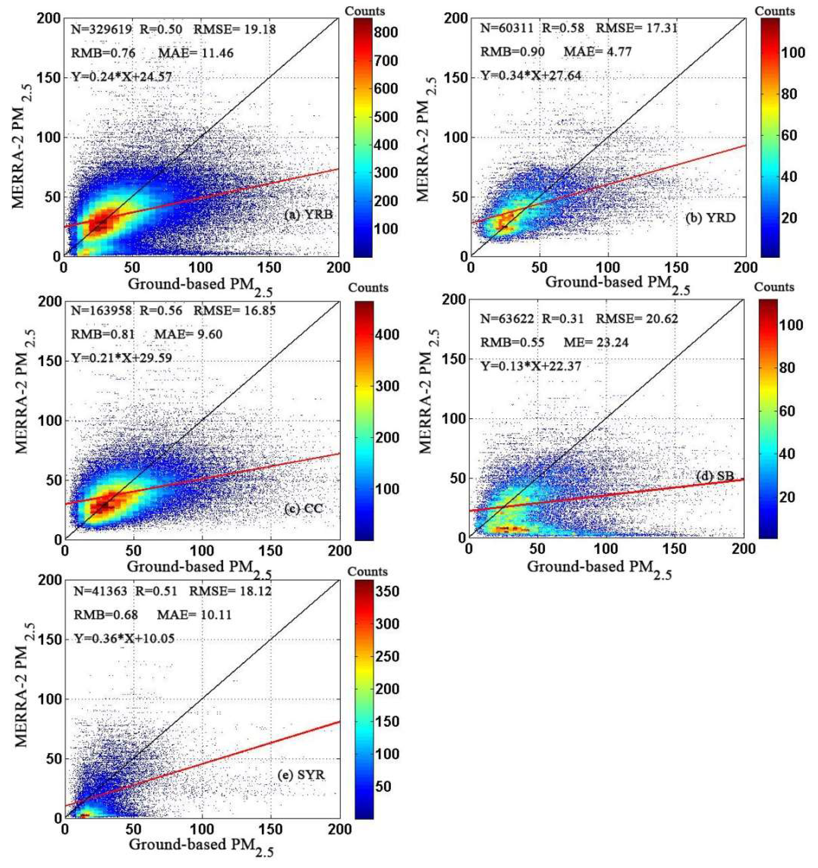
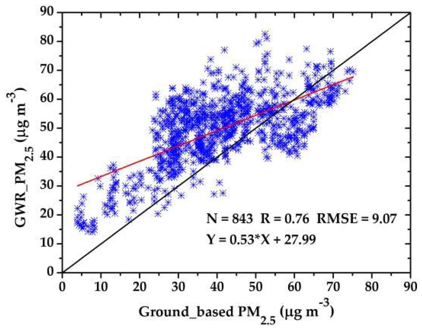
3.1. Ground-Based Verification of MERRA-2 PM2.5
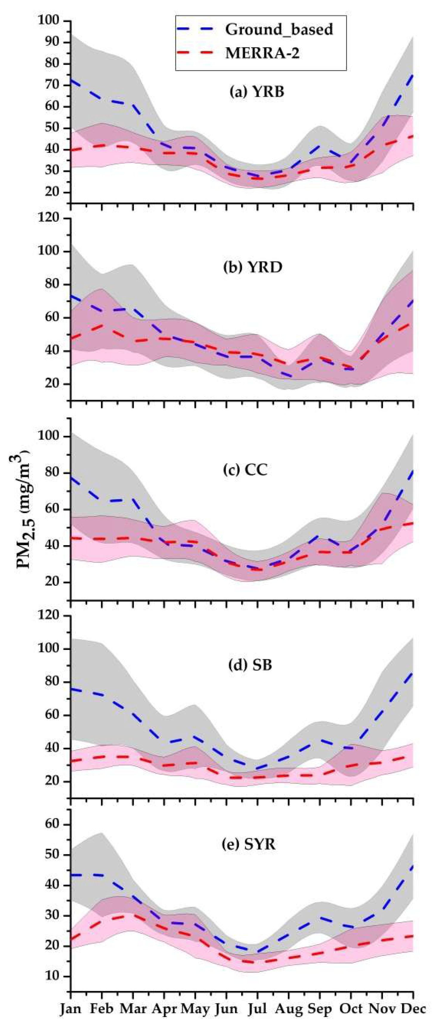
3.1.1. Regional and Seasonal Comparisons between MERRA-2 and Ground PM2.5
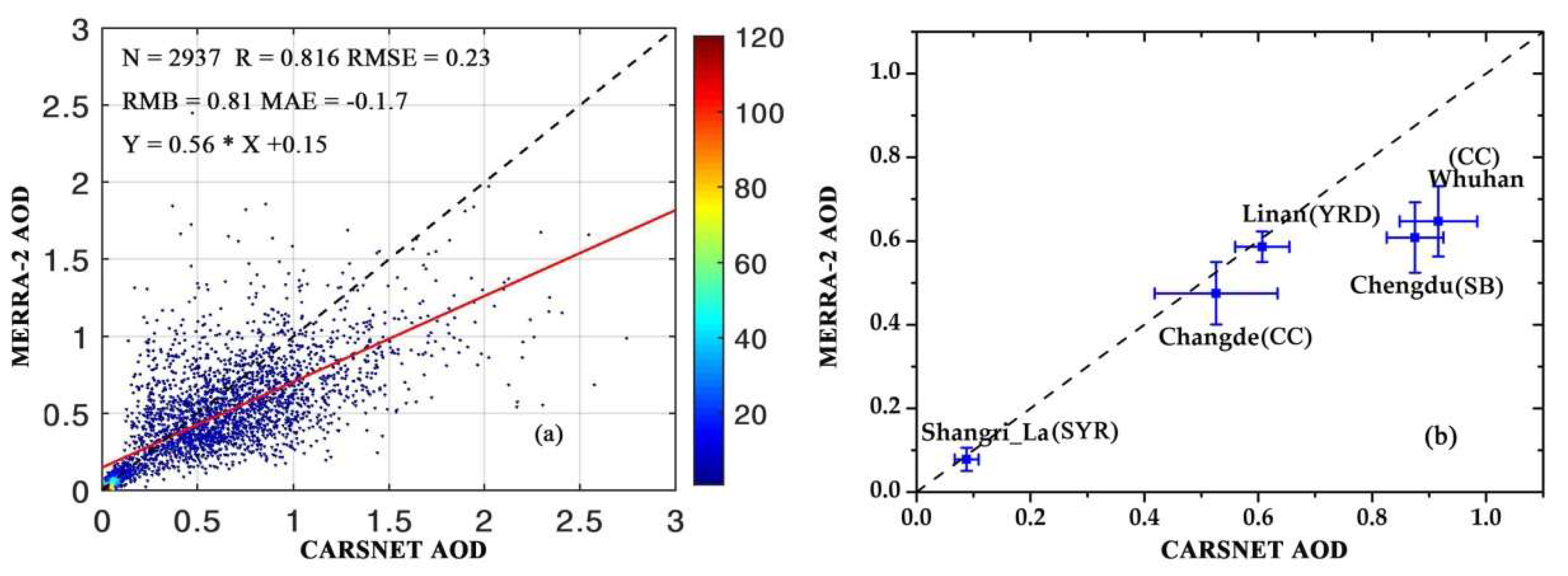
3.1.2. Impact of AOD Assimilation
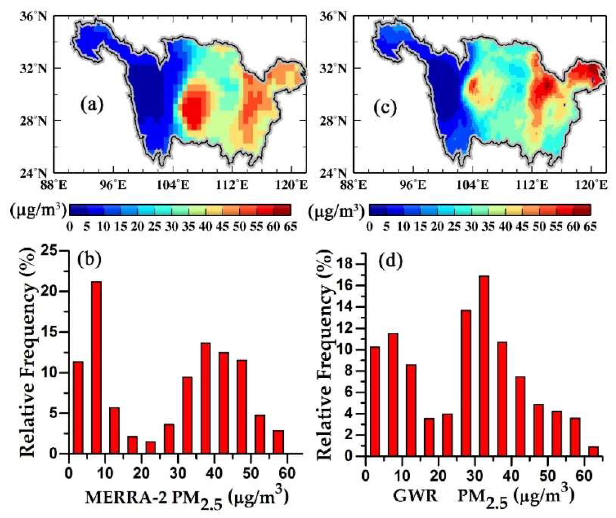
3.2. Spatiotemporal Distribution of MERRA-2 PM2.5 Components
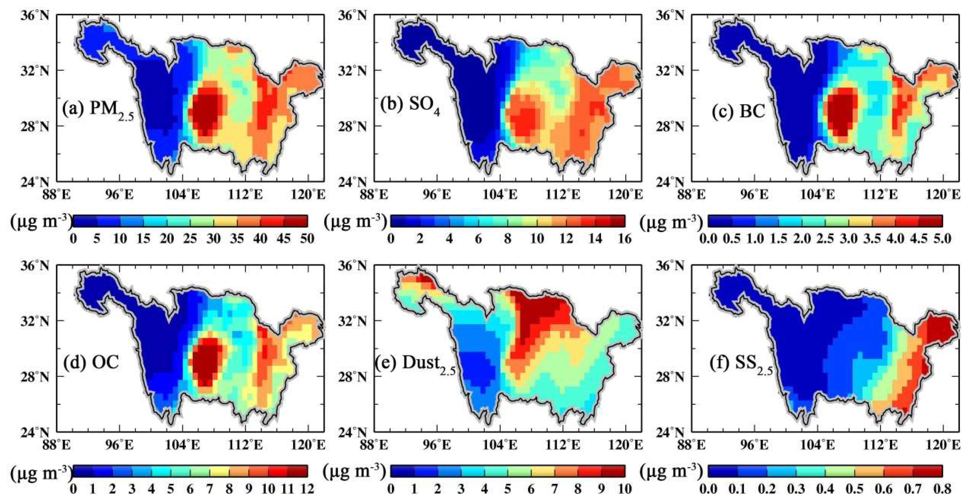
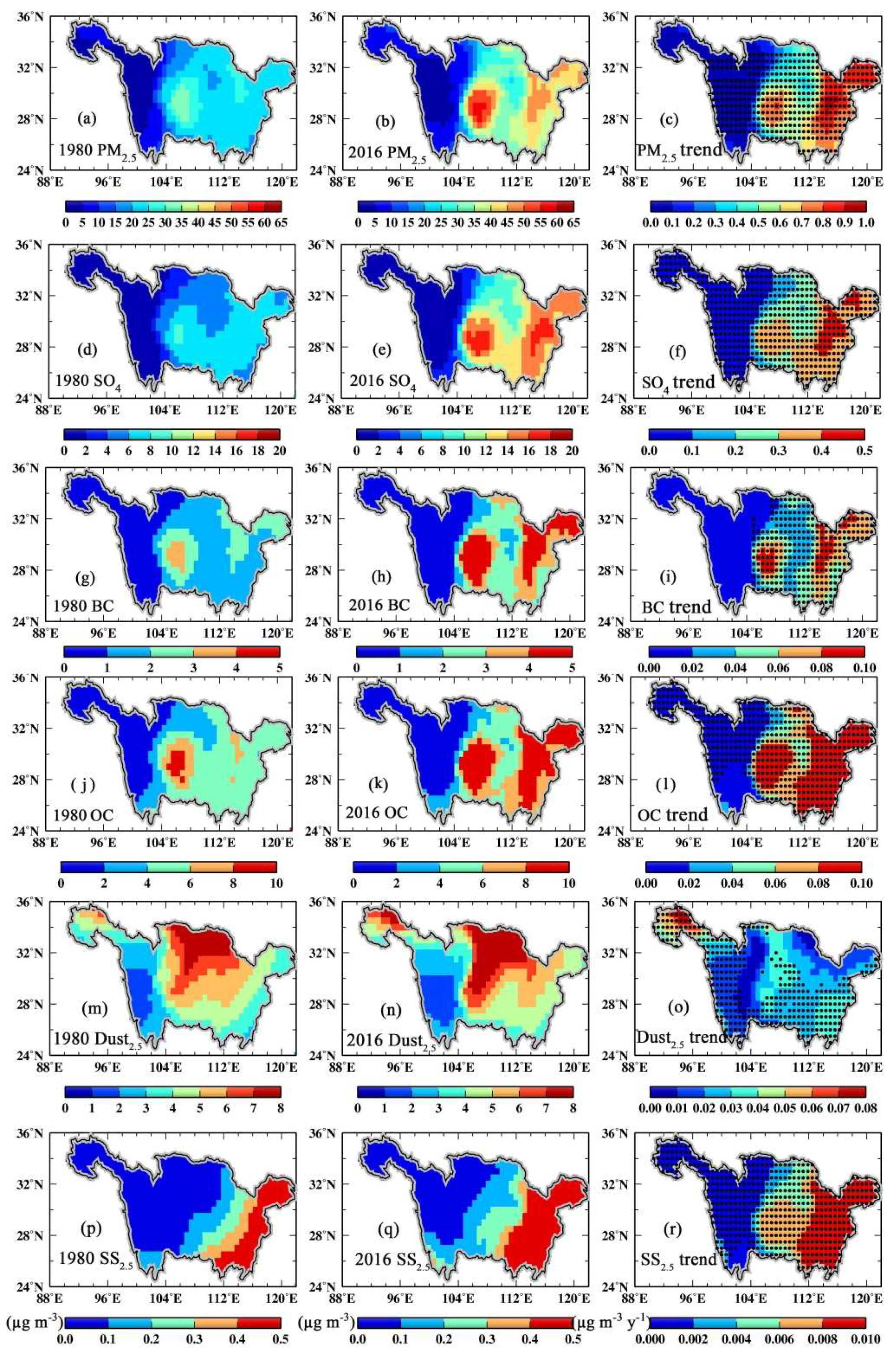
3.2.1. Annual Mean Distribution in MERRA-2 PM2.5 Components
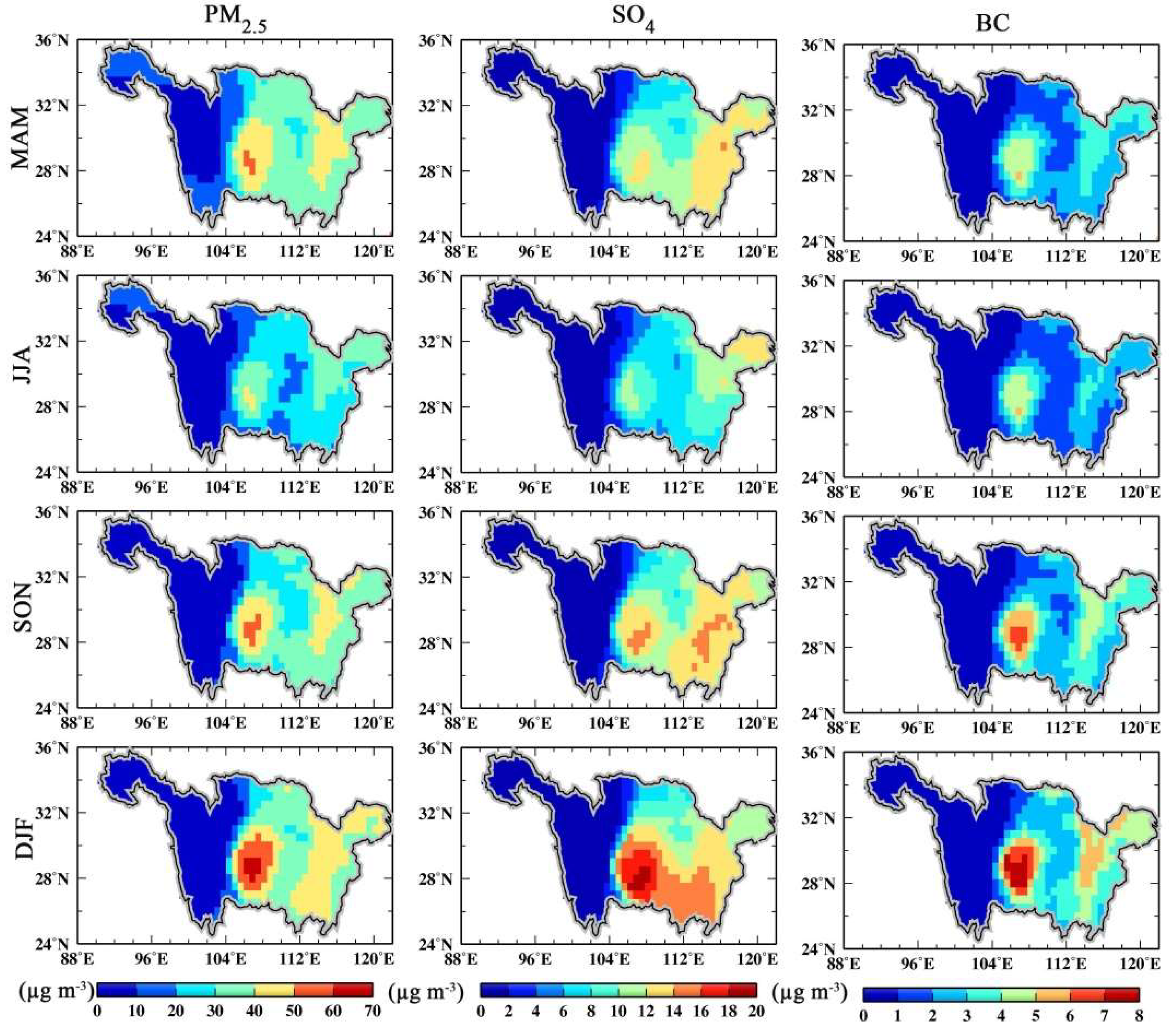
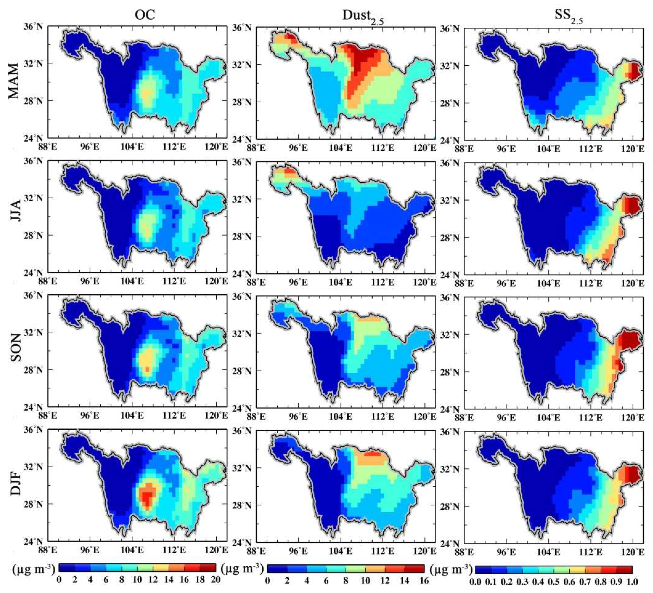
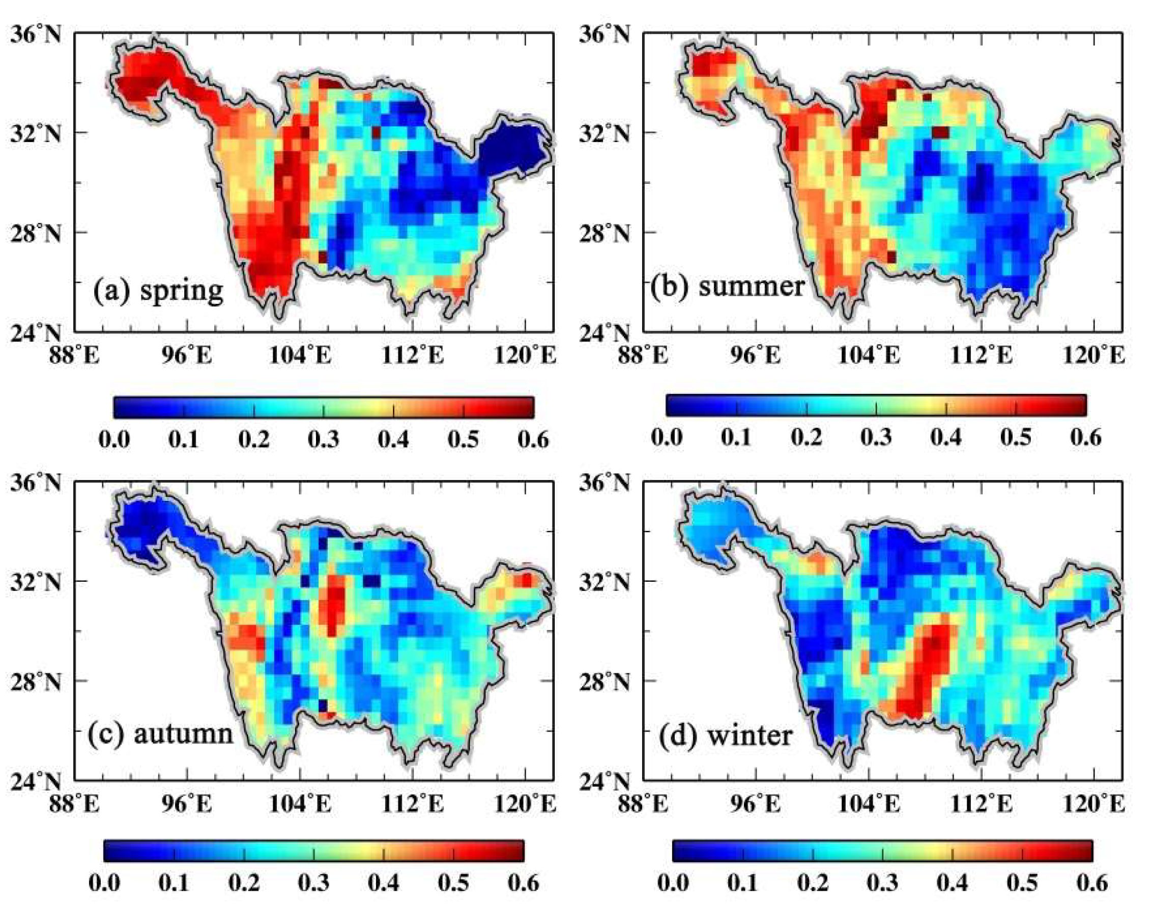
3.2.2. Seasonal Variation in MERRA-2 PM2.5 Components
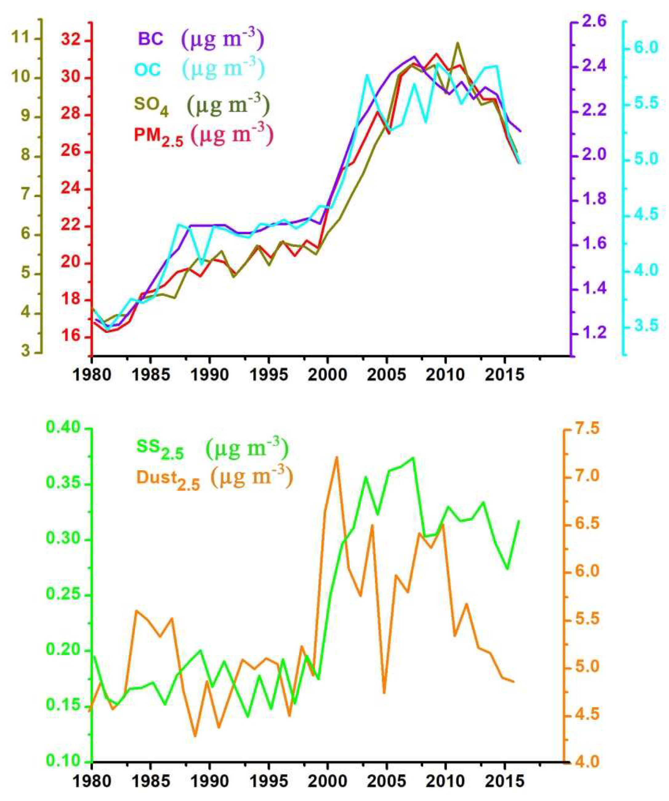
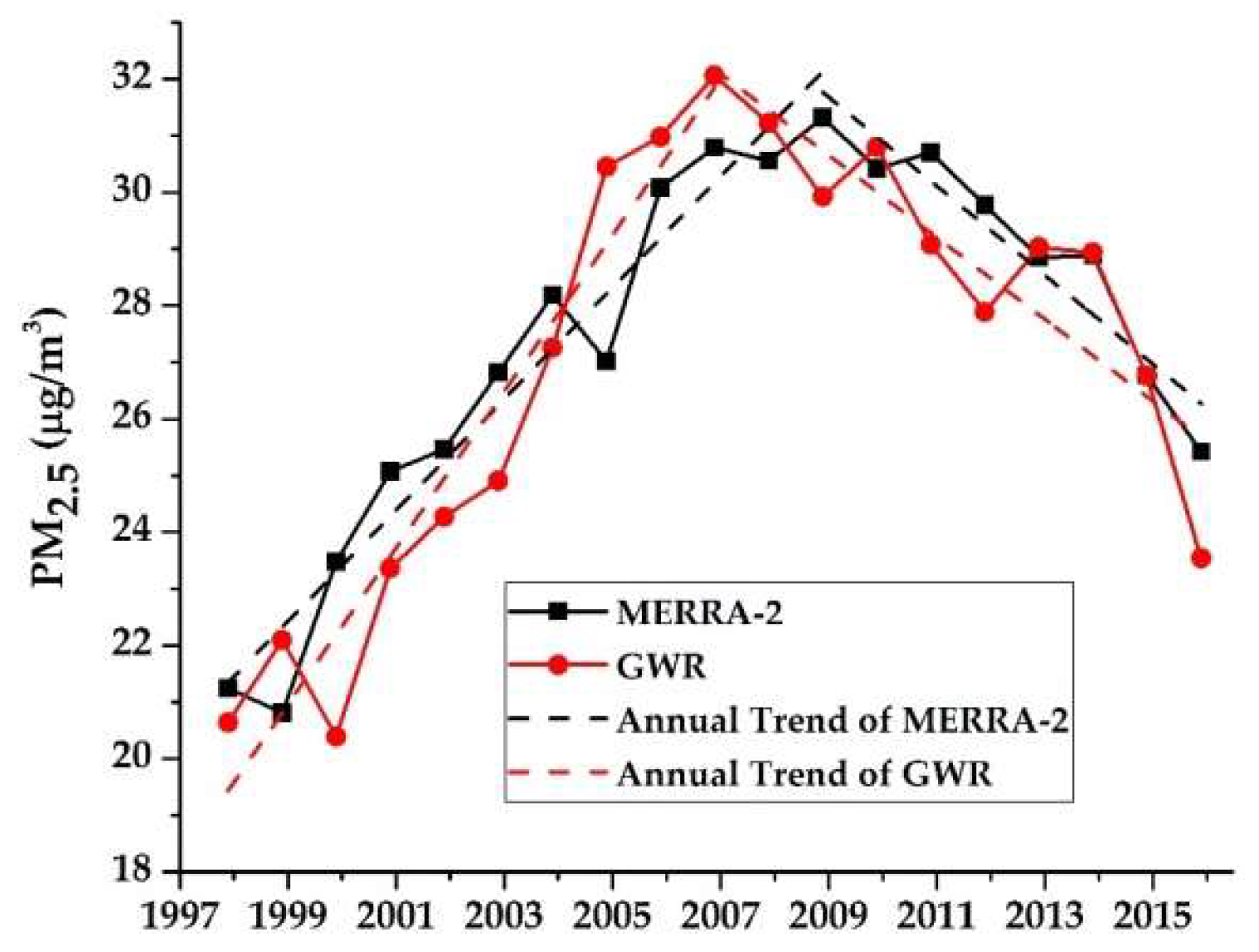
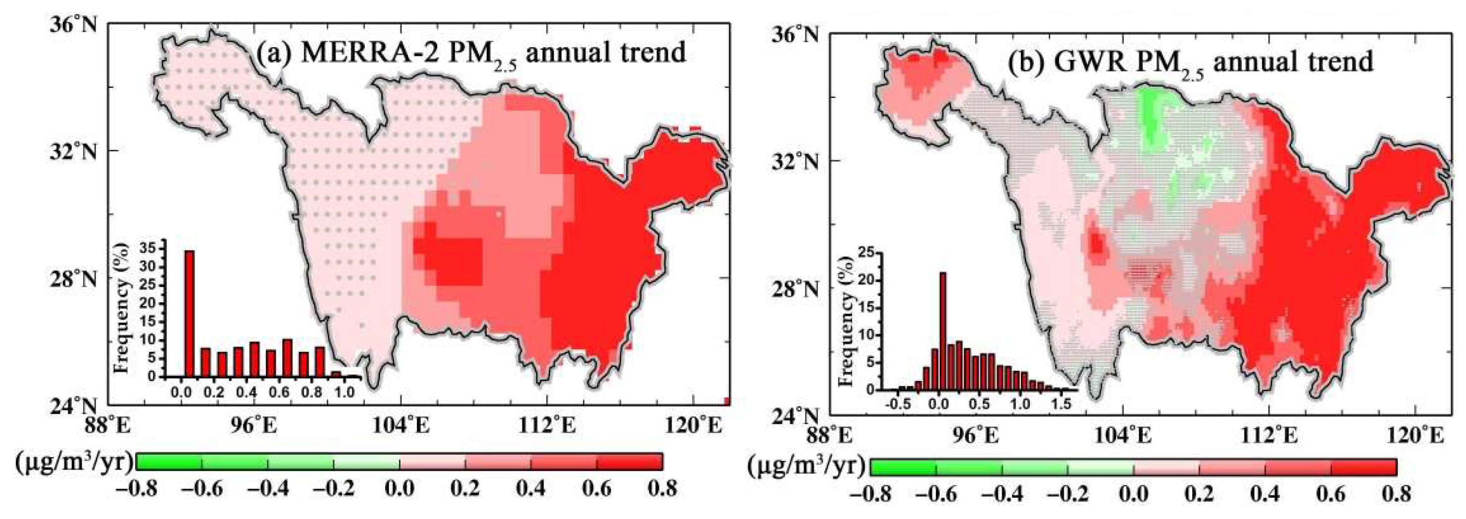
3.2.3. Long-Term Trends of MERRA-2 PM2.5 Components
4. Discussion
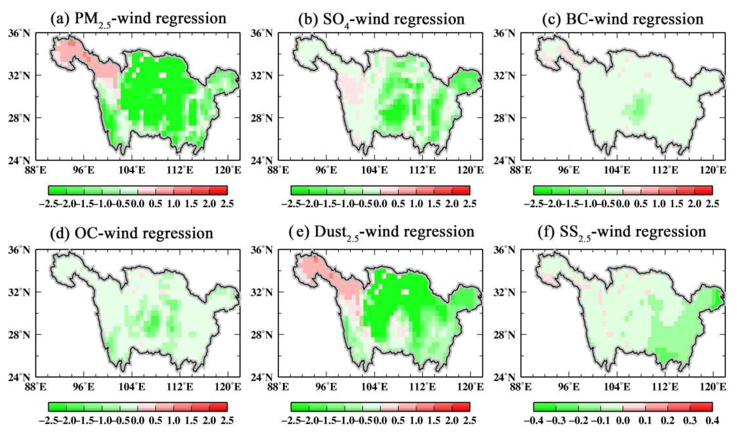
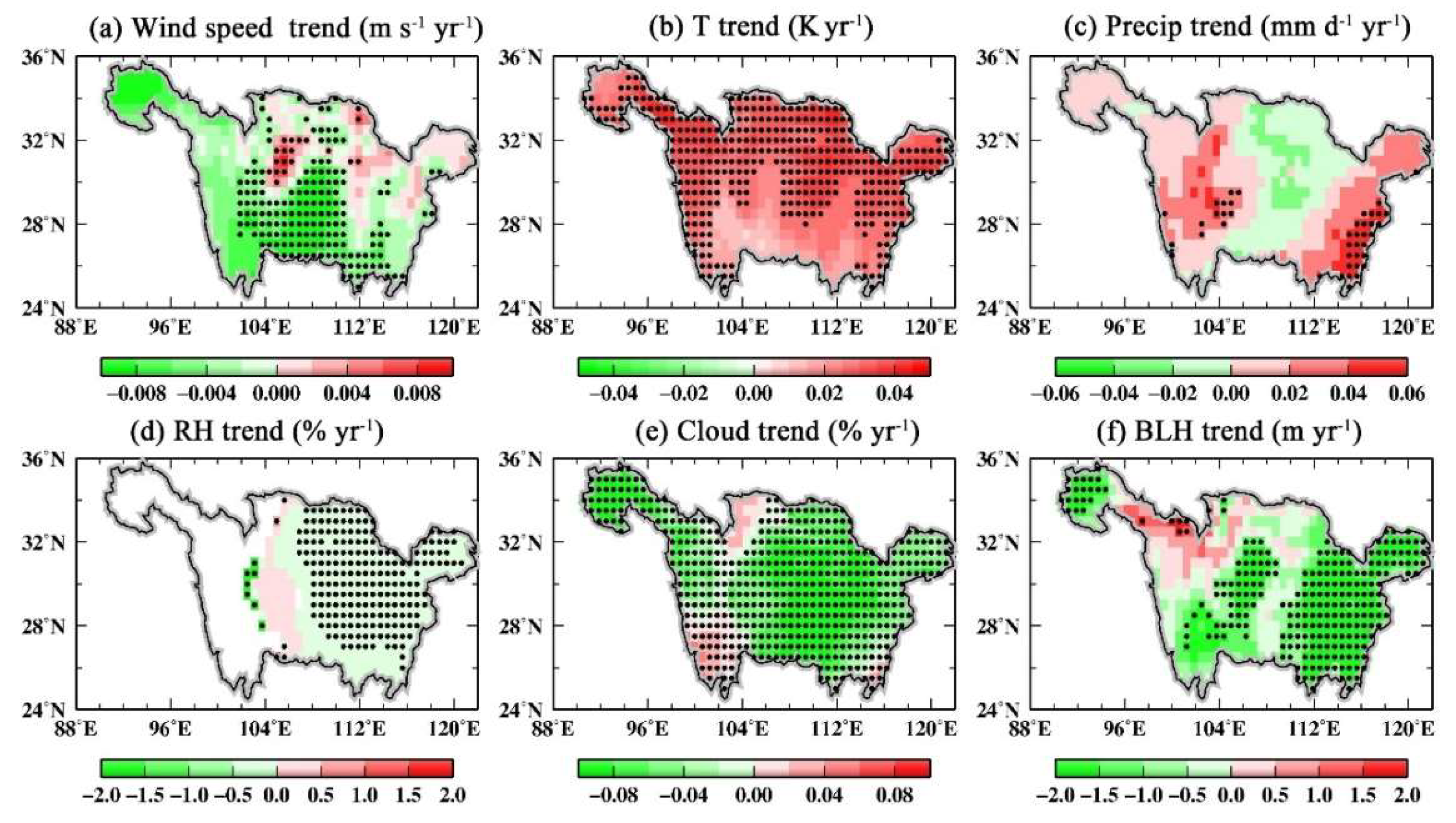
4.1. Sensitivity of PM2.5 Components to Surface Wind Speed
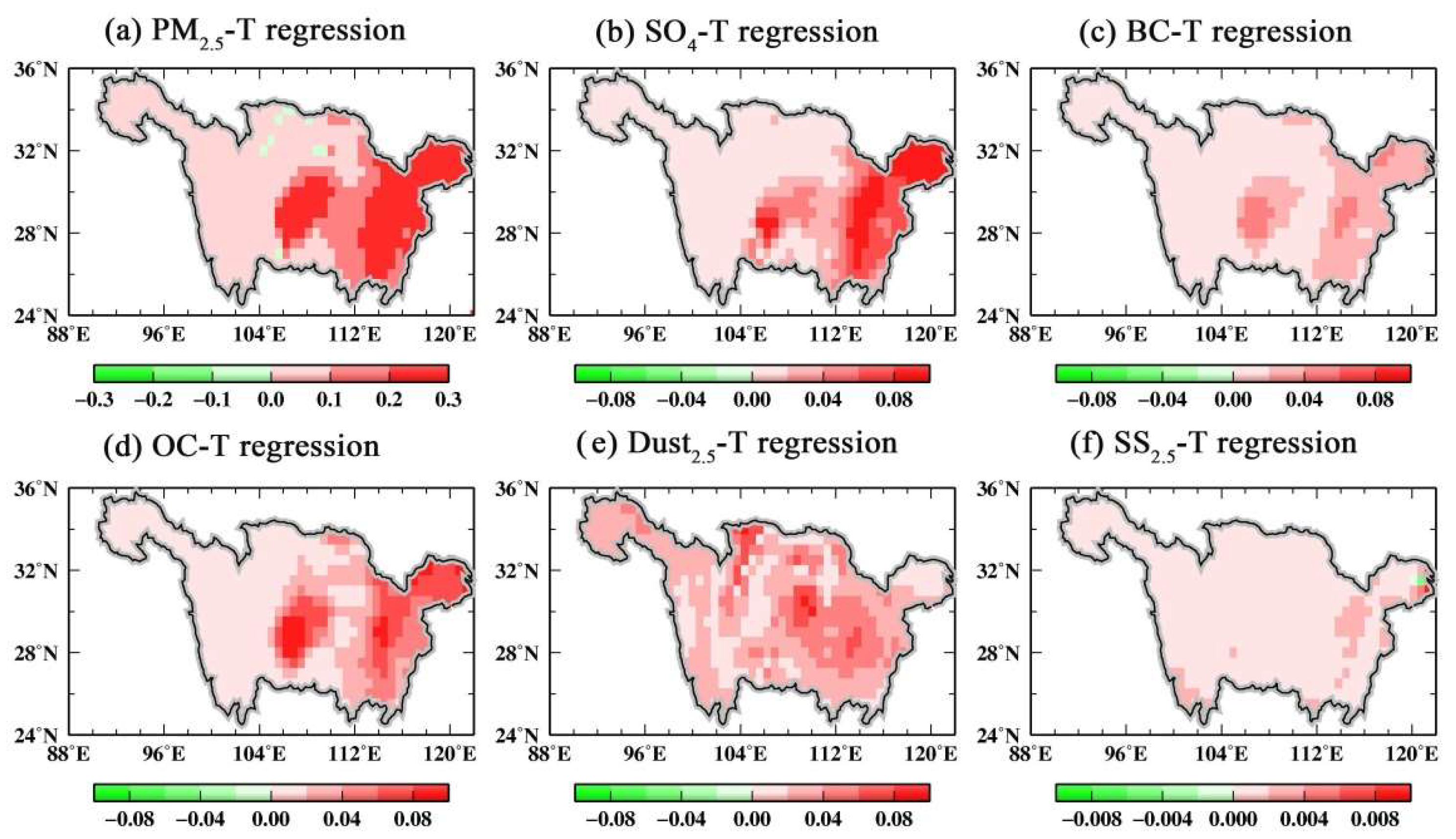
4.2. Sensitivity of PM2.5 Components to Surface Temperature
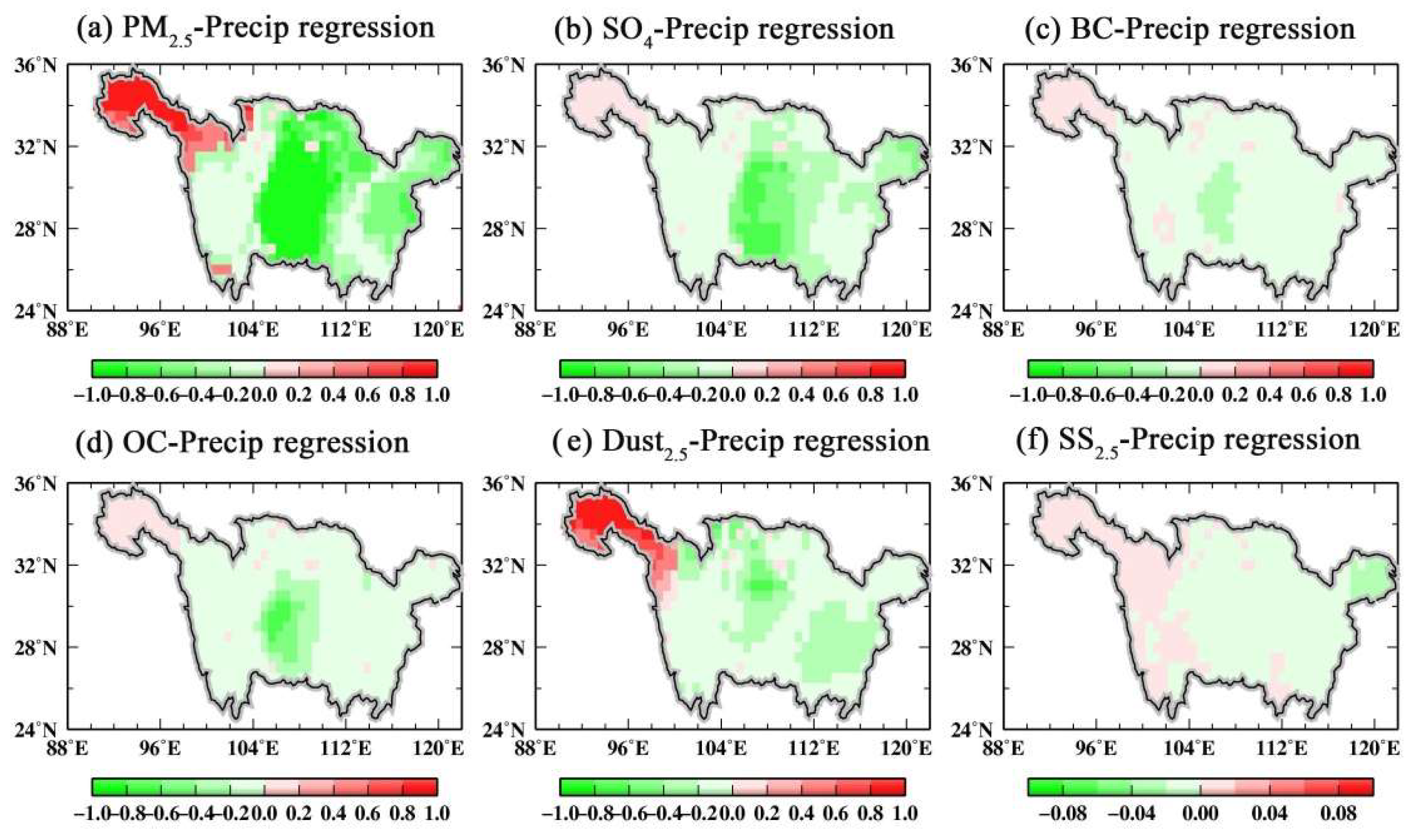
4.3. Sensitivity of PM2.5 Components to Precipitation
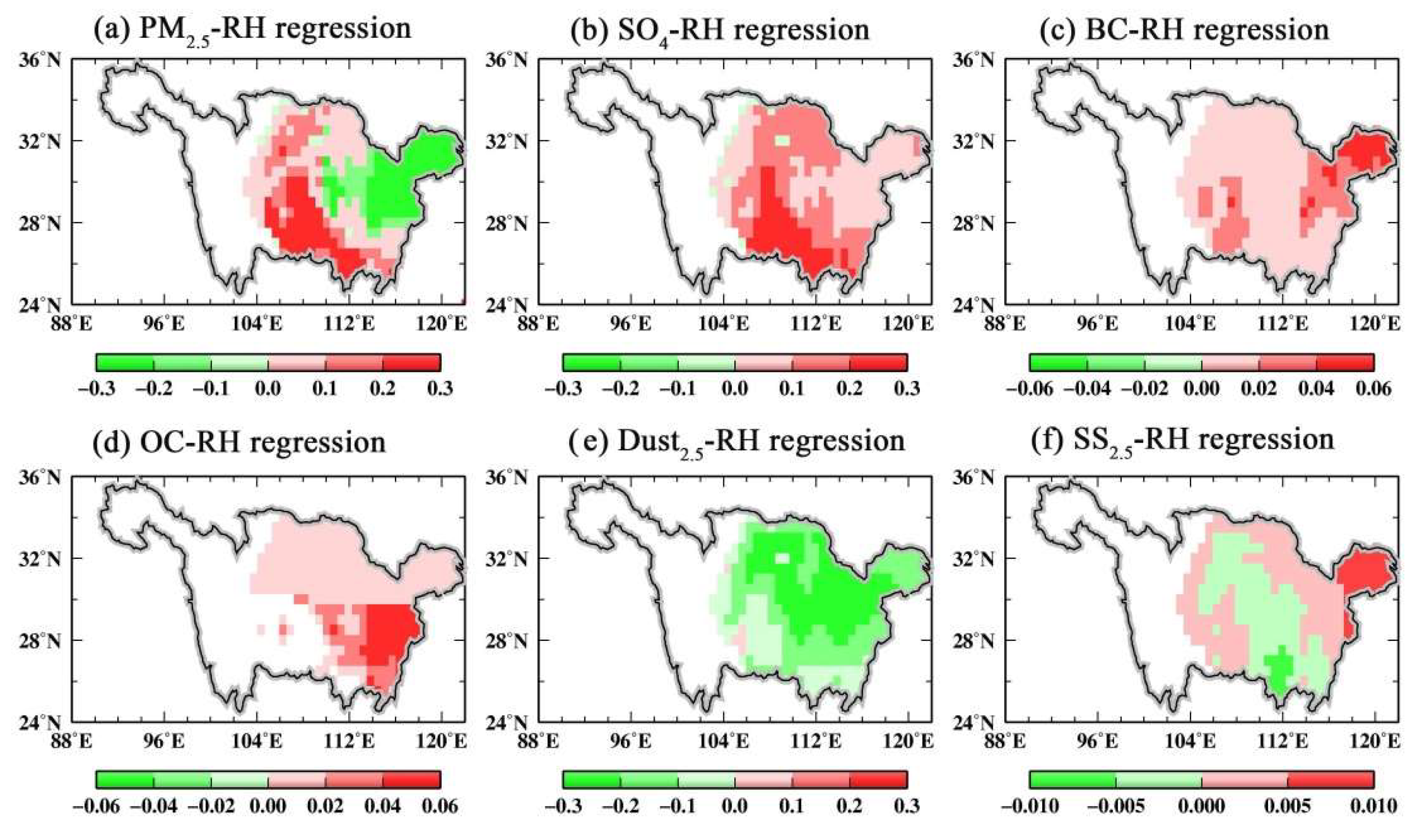
4.4. Sensitivity of PM2.5 Components to Relative Humidity
4.5. Sensitivity of PM2.5 Components to Total Cloud Cover
4.6. Sensitivity of PM2.5 Components to Boundary Layer Height
5. Conclusions
Author Contributions
Funding
Conflicts of Interest
Appendix A


| T | Wind | Precip | RH | Cloud | BLH | |
|---|---|---|---|---|---|---|
| T | 1 | |||||
| Wind | 0.514 | 1 | ||||
| Precip | −0.202 | −0.089 | 1 | |||
| RH | 0.074 | −0.334 | 0.359 | 1 | ||
| Cloud | 0.274 | 0.26 | 0.519 * | 0.28 | 1 | |
| BLH | −0.559 | −0.543 | −0.222 | 0.351 | −0.416 | 1 |


| Regression Coefficients | Annual trends in Meteorological Variables | Theoretical Annual Trends in PM2.5 |
|---|---|---|
| β1 (−2.42 µg m−3 m−1 s) | Wind (0.05 m s−1) | 0.12 µg m−3 |
| β2 (0.11 µg m−3 K−1) | T (0.03 K) | 0.003 µg m−3 |
| β3 (−0.34 µg m−3 mm−1 day) | Precip (0.02 mm day−1) | 0.007 µg m−3 |
| β4 (0.05 µg m−3 %−1) | RH (−0.16%) | −0.008 µg m−3 |
| β5 (−0.07 µg m−3 %−1) | Cloud (−0.05%) | 0.0004 µg m−3 |
| β6 (0.006 µg m−3 m−1) | BLH (−0.98 m) | 0.006 µg m−3 |
References
- IPCC. Climate change 2013: the physical science basis. In Contribution of Working Group I to the Fifth Assessment Report of the Intergovernmental Panel on Climate Change; Stocker, T.F., Qin, D., Plattner, G.-K., Tignor, M., Allen, S.K., Boschung, J., Nauels, A., Xia, Y., Bex, V., Midgley, P.M., Eds.; Cambridge University Press: Cambridge, UK; New York, NY, USA, 2013; p. 1535. [Google Scholar]
- Guo, J.; Xia, F.; Zhang, Y.; Liu, H.; Li, J.; Lou, M.; Zhai, P. Impact of diurnal variability and meteorological factors on the PM2.5-AOD relationship: Implications for PM2.5 remote sensing. Environ. Pollut. 2017, 221, 94–104. [Google Scholar] [CrossRef] [PubMed]
- He, J.; Gong, S.; Yu, Y.; Yu, L.; Wu, L.; Mao, H.; Li, R. Air pollution characteristics and their relation to meteorological conditions during 2014–2015 in major Chinese cities. Environ. Pollut. 2017, 223, 484–496. [Google Scholar] [CrossRef] [PubMed]
- Zhang, M.; Wang, L.; Gong, W.; Ma, Y.; Liu, B. Aerosol optical properties and direct radiative effects over Central China. Remote Sens. 2017, 9, 997. [Google Scholar] [CrossRef]
- Zhang, M.; Ma, Y.; Wang, L.; Gong, W.; Hu, B.; Shi, Y. Spatial-temporal characteristics of aerosol loading over the Yangtze River Basin during 2001–2015. Int. J. Climatol. 2018, 38, 2138–2152. [Google Scholar] [CrossRef]
- Qin, W.; Liu, Y.; Wang, L.; Lin, A.; Xia, X.; Che, H.; Zhang, M. Characteristic and driving factors of aerosol optical depth over mainland China during 1980–2017. Remote Sens. 2018, 10, 1064. [Google Scholar] [CrossRef]
- Lelieveld, J.; Evans, J.S.; Fnais, M.; Giannadaki, D.; Pozzer, A. The contribution of outdoor air pollution sources to premature mortality on a global scale. Nature 2015, 525, 367–371. [Google Scholar] [CrossRef] [PubMed]
- He, L.; Wang, L.; Lin, A.; Zhang, M.; Bilal, M.; Tao, M. Aerosol Optical Properties and Associated Direct Radiative Forcing over the Yangtze River Basin during 2001–2015. Remote Sens. 2017, 9, 746. [Google Scholar] [CrossRef]
- He, L.; Wang, L.; Lin, A.; Zhang, M.; Bilal, M.; Wei, J. Performance of the NPP–VIIRS and aqua–MODIS Aerosol Optical Depth Products over the Yangtze River Basin. Remote Sens. 2018, 10, 117. [Google Scholar] [CrossRef]
- He, L.; Wang, L.; Lin, A.; Zhang, M.; Xia, X.; Tao, M.; Zhou, H. What drives changes in aerosol properties over the Yangtze River Basin in past four decades? Atmos. Environ. 2018, 190, 269–283. [Google Scholar] [CrossRef]
- Wang, L.; Gong, W.; Xia, X.; Zhu, J.; Li, J.; Zhu, Z. Long–term observations of aerosol optical properties at Wuhan, an urban site in Central China. Atmos. Environ. 2015, 101, 94–102. [Google Scholar] [CrossRef]
- Che, H.; Xia, X.; Goloub, P.; Holben, B.; Zhao, H.; Wang, Y.; Zhang, X.; Wang, H.; Blarel, L.; Damiri, B. Ground-based aerosol climatology of China: aerosol optical depths from the China Aerosol Remote Sensing Network (CARSNET) 2002-2013. Atmos. Chem. Phys. 2015, 15, 7619–7652. [Google Scholar] [CrossRef]
- Wei, J.; Sun, L. Comparison and evaluation of different modis aerosol optical depth products over the beijing-tianjin-hebei region in china. IEEE J-STARS 2016, PP(99), 1–10. [Google Scholar] [CrossRef]
- Wang, L.; Lu, Y.; Zou, L.; Feng, L.; Wei, J.; Qin, W.; Niu, Z. Prediction of diffuse solar radiation based on multiple variables in China. Renew. Sust. Energ. Rev. 2019, 103, 151–216. [Google Scholar] [CrossRef]
- Feng, L.; Lin, A.; Wang, L.; Qin, W.; Gong, W. Evaluation of sunshine-based models for predicting diffuse solar radiation in China. Renew. Sust. Energ. Rev. 2018, 94, 168–182. [Google Scholar] [CrossRef]
- Feng, L.; Qin, W.; Wang, L.; Lin, A.; Zhang, M. Comparison of Artificial Intelligence and Physical Models for Forecasting Photosynthetically-Active Radiation. Remote Sens. 2018, 10, 1855. [Google Scholar] [CrossRef]
- Wang, L.; Chen, Y.; Niu, Y.; Salazar, G.A.; Gong, W. Analysis of atmospheric turbidity in clear skies at Wuhan, Central China. J. Earth Sci. 2017, 28, 729–738. [Google Scholar] [CrossRef]
- Wang, L.; Kisi, O.; Zounemat-Kermani, M.; Zhu, Z.; Gong, W.; Niu, Z.; Liu, Z. Prediction of solar radiation in China using different adaptive neuro-fuzzy methods and M5 model tree. Int. J. Climatol. 2017, 37, 1141–1155. [Google Scholar] [CrossRef]
- Wang, L.; Kisi, O.; Zounemat-Kermani, M.; Salazar, G.A.; Zhu, Z.; Gong, W. Solar radiation prediction using different techniques: model evaluation and comparison. Renew. Sust. Energ. Rev. 2016, 61, 384–397. [Google Scholar] [CrossRef]
- Zhang, M.; Ma, Y.; Gong, W.; Wang, L.; Xia, X.; Che, H.; Hu, B.; Liu, B. Aerosol radiative effect in UV, VIS, NIR, and SW spectra under haze and high-humidity urban conditions. Atmos. Environ. 2017, 166, 9–21. [Google Scholar] [CrossRef]
- Guo, J.; He, J.; Liu, H.; Miao, Y.; Liu, H.; Zhai, P. Impact of various emission control schemes on air quality using WRF-Chem during APEC China 2014. Atmos. Environ. 2016, 140, 311–319. [Google Scholar] [CrossRef]
- Ren, Y.; Li, H.; Meng, F.; Wang, G.; Zhang, H.; Yang, T.; Li, W.; Ji, Y.; Bi, F.; Wang, X. Impact of emission controls on air quality in Beijing during the 2015 China Victory Day Parade: Implication from organic aerosols. Atmos. Environ. 2019, 198, 207–214. [Google Scholar] [CrossRef]
- Larkin, A.; Van Donkelaar, A.; Geddes, J.A.; Martin, R.V.; Hystad, P. Relationships between changes in urban characteristics and air quality in East Asia from 2000 to 2010. Environ. Sci. Technol. 2016, 50, 9142–9149. [Google Scholar] [CrossRef] [PubMed]
- Li, T.; Wang, Y.; Zhao, D. Environmental Kuznets curve in China: new evidence from dynamic panel analysis. Energy Policy 2016, 91, 138–147. [Google Scholar] [CrossRef]
- Liu, Y.; Zhou, Y.; Wu, W. Assessing the impact of population, income and technology on energy consumption and industrial pollutant emissions in China. Appl. Energy 2015, 155, 904–917. [Google Scholar] [CrossRef] [Green Version]
- Tai, A.P.; Mickley, L.J.; Jacob, D.J. Correlations between fine particulate matter (PM2.5) and meteorological variables in the United States: Implications for the sensitivity of PM2.5 to climate change. Atmos. Environ. 2010, 44, 3976–3984. [Google Scholar] [CrossRef]
- Westervelt, D.M.; Horowitz, L.W.; Naik, V.; Tai, A.P.K.; Fiore, A.M.; Mauzerall, D.L. Quantifying PM2.5-meteorology sensitivities in a global climate model. Atmos. Environ. 2016, 142, 43–56. [Google Scholar] [CrossRef]
- Harrison, R.M.; Laxen, D.; Moorcroft, S.; Laxen, K. Processes affecting concentrations of fine particulate matter (PM2.5) in the UK atmosphere. Atmos. Environ. 2012, 46, 115–124. [Google Scholar] [CrossRef]
- Kassomenos, P.A.; Vardoulakis, S.; Chaloulakou, A.; Paschalidou, A.K.; Grivas, G.; Borge, R.; Lumbreras, J. Study of PM10 and PM2.5 levels in three European cities: Analysis of intra and inter urban variations. Atmos. Environ. 2014, 87, 153–163. [Google Scholar] [CrossRef]
- Munir, S.; Habeebullah, T.M.; Mohammed, A.M.; Morsy, E.A.; Rehan, M.; Ali, K. Analysing PM2.5 and its association with PM10 and meteorology in the arid climate of Makkah, Saudi Arabia. Aerosol Air Qual. Res. 2017, 17, 453–464. [Google Scholar] [CrossRef]
- Wang, X.; Dickinson, R.E.; Su, L.; Zhou, C.; Wang, K. PM2.5 pollution in China and how it has been exacerbated by terrain and meteorological conditions. Bull. Am. Meteoro. Soc. 2018, 99, 105–119. [Google Scholar] [CrossRef]
- Chen, Y.; Schleicher, N.; Fricker, M.; Cen, K.; Liu, X.-L.; Kaminski, U.; Yu, Y.; Wu, X.-F.; Norra, S. Long-term variation of black carbon and PM2.5 in Beijing, China with respect to meteorological conditions and governmental measures. Environ. Pollut. 2016, 212, 269–278. [Google Scholar] [CrossRef] [PubMed]
- Yang, Q.; Yuan, Q.; Li, T.; Shen, H.; Zhang, L. The relationships between PM2.5 and meteorological factors in China: Seasonal and regional variations. Int. J. Environ. Res. Public Health 2017, 14, 1510. [Google Scholar]
- Lin, Y.; Zou, J.; Yang, W.; Li, C.Q. A review of recent advances in research on PM2.5 in China. Int. J. Environ. Res. Public Health 2018, 15, 438. [Google Scholar] [CrossRef] [PubMed]
- Li, L.; Qian, J.; Ou, C.Q.; Zhou, Y.X.; Guo, C.; Guo, Y. Spatial and temporal analysis of Air Pollution Index and its timescale-dependent relationship with meteorological factors in Guangzhou, China, 2001–2011. Environ. Pollut. 2014, 190, 75–81. [Google Scholar] [CrossRef] [PubMed]
- Zhang, T.; Zhu, Z.; Gong, W.; Zhu, Z.; Sun, K.; Wang, L.; Xu, K. Estimation of ultrahigh resolution PM2.5 concentrations in urban areas using 160 m Gaofen-1 AOD retrievals. Remote Sens. Environ. 2018, 216, 91–104. [Google Scholar] [CrossRef]
- Buchard, V.; da Silva, A.M.; Randles, C.A.; Colarco, P.; Ferrare, R.; Hair, J.; Winker, D. Evaluation of the surface PM2.5 in Version 1 of the NASA MERRA Aerosol Reanalysis over the United States. Atmos. Environ. 2016, 125, 100–111. [Google Scholar] [CrossRef]
- Randles, C.A.; Da Silva, A.M.; Buchard, V.; Colarco, P.R.; Darmenov, A.; Govindaraju, R.; Shinozuka, Y. The MERRA-2 aerosol reanalysis, 1980 onward. Part I: System description and data assimilation evaluation. J. Climate 2017, 30, 6823–6850. [Google Scholar] [CrossRef] [PubMed]
- Buchard, V.; Randles, C.A.; da Silva, A.M.; Darmenov, A.; Colarco, P.R.; Govindaraju, R.; Yu, H. The MERRA-2 aerosol reanalysis, 1980 onward. Part II: Evaluation and case studies. J. Climate 2017, 30, 6851–6872. [Google Scholar] [CrossRef]
- Song, Z.; Fu, D.; Zhang, X.; Wu, Y.; Xia, X.; He, J.; Che, H. Diurnal and seasonal variability of PM2.5 and AOD in North China plain: Comparison of MERRA-2 products and ground measurements. Atmos. Environ. 2018, 191, 70–78. [Google Scholar] [CrossRef]
- Van Donkelaar, A.; Martin, R.V.; Spurr, R.J.D.; Drury, E.; Remer, L.A.; Levy, R.C.; Wang, J. Optimal estimation for global ground-level fine particulate matter concentrations. J. Geophys. Res. Atmos. 2013, 118, 5621–5636. [Google Scholar] [CrossRef] [Green Version]
- Van Donkelaar, A.; Martin, R.V.; Brauer, M.; Kahn, R.; Levy, R.; Verduzco, C.; Villeneuve, P.J. Global estimates of ambient fine particulate matter concentrations from satellite-based aerosol optical depth: development and application. Environ. Health Perspect. 2010, 118, 847–855. [Google Scholar] [CrossRef] [PubMed]
- Huang, J.; Kondragunta, S.; Laszlo, I.; Liu, H.; Remer, L.A.; Zhang, H.; Petrenko, M. Validation and expected error estimation of Suomi-NPP VIIRS aerosol optical thickness and Ångström exponent with AERONET. J. Geophys. Res. Atmos. 2016, 121, 7139–7160. [Google Scholar] [CrossRef]
- Peng, S.-S.; Piao, S.; Zeng, Z.; Ciais, P.; Zhou, L.; Li, L.Z.; Zeng, H. Afforestation in China cools local land surface temperature. Proc. Natl. Acad. Sci. USA 2014, 121, 2915–2919. [Google Scholar] [CrossRef] [PubMed]
- Dawson, J.P.; Adams, P.J.; Pandis, S.N. Sensitivity of PM2.5 to climate in the Eastern US: a modeling case study. Atmos. Chem. Phys. 2007, 7, 4295–4309. [Google Scholar] [CrossRef]
- Zhou, H.; Luo, Z.; Zhou, Z.; Li, Q.; Zhong, B.; Lu, B.; Hsu, H. Impact of different kinematic empirical parameters processing strategies on temporal gravity field model determination. J. Geophys. Res. Solid Earth 2018. [Google Scholar] [CrossRef]
- Zhou, H.; Luo, Z.; Tangdamrongsub, N.; Zhou, Z.; He, L.; Xu, C.; Li, Q.; Wu, Y. Identifying Flood Events over the Poyang Lake Basin Using Multiple Satellite Remote Sensing Observations, Hydrological Models and In Situ Data. Remote Sens. 2018, 10, 713. [Google Scholar] [CrossRef]
- Zhou, H.; Luo, Z.; Tangdamrongsub, N.; Wang, L.; He, L.; Xu, C.; Li, Q. Characterizing drought and flood events over the Yangtze River Basin using the HUST-Grace2016 solution and ancillary data. Remote Sens. 2017, 9, 1100. [Google Scholar] [CrossRef]


| Study Areas | Methods | Meteorological Variables | Pollution Indicators | Main Conclusions |
|---|---|---|---|---|
| United states (1998–2008) [26] | Multiple linear regression (MLR) | Surface temperature, precipitation, total cloud cover, wind speed, wind direction and relative humidity | PM2.5, SO4, OC, EC * | Daily meteorological variables could explain up to 50% changes of PM2.5 in the USA. |
| Global scale (2005–2016) [27] | Chemistry-climate model | Surface temperature, precipitation, total cloud cover, wind speed, relative humidity and pressure | PM2.5 | PM2.5 concentrations were most sensitive to surface temperature, wind speed and precipitation. |
| United Kingdom (2009) [28] | Regression analyses | Wind speed and direction | PM10, PM2.5, NOx * | PM2.5 concentrations exhibited a stronger correlation with easterly winds from the European mainland than with the local traffic sources. |
| Three European cities (2005–2015) [29] | Principal component and regression analyses | Wind velocity, temperature, relative humidity, precipitation, solar radiation and atmospheric pressure | PM10, PM2.5 | Local meteorological conditions had a significant impact on air pollutions. |
| Europe, US, China (2013–2016) [30] | MLR | Air stagnation event (i.e., daily 10-m wind speed < 3.2 m s−1, 500-hPa tropospheric wind speed < 13m s−1 and no precipitation) | PM2.5 | Compared to no-stagnation conditions, air stagnation events in winter could increase PM2.5 concentrations in the United States, Europe and China by 46%, 68% and 60%, respectively. |
| Saudi Arabia (2014–2015) [31] | MLR | Relative humidity, wind speed and temperature | PM2.5, PM10 | Both PM10 and PM2.5 were anti-correlated with relative humidity, but positively related to wind speed and temperature. |
| Beijing China (2005–2013) [32] | MLR | Relative humidity and wind speed | Black carbon (BC) | High BC concentrations were usually related to poor visibility and low wind speed. |
| China (2013–2014) [33] | Multivariate analysis | Relative humidity, wind speed, surface pressure and temperature | PM2.5 | PM2.5 was significantly correlated with meteorological conditions in China. |
| Spatial Resolution | Temporal Coverage | Data Source | ||
|---|---|---|---|---|
| PM2.5 | MERRA-2 * | 0.05° × 0.625° | daily\1980–2017 | http://disc.sci.gsfc.nasa.gov/mdisc/ |
| GWR * | 0.01° × 0.01° | daily\1998–2017 | http://fizz.phys.dal.ca/~atmos/martin/?page_id=140 | |
| Ground | \ | daily\2015–2016 | http://113.108.142.147:20035/emcpublish/ | |
| AOD * | MERRA-2 | 0.05° × 0.625° | daily\2013–2016 | http://disc.sci.gsfc.nasa.gov/mdisc/ |
| CARSNET * | \ | daily\2013–2016 | \ | |
| Terra, Aqua | 0.01° × 0.01° | daily\2016 | https://ladsweb.modaps.eosdis.nasa.gov/search/ | |
| Meteorological factors | MERRA-2 | 0.05° × 0.625° | daily\1980–2017 | http://disc.sci.gsfc.nasa.gov/mdisc/ |
| PM2.5 | SO4 | BC | OC | Dust2.5 | SS2.5 | |
|---|---|---|---|---|---|---|
| Annual | 23.43 | 6.80 | 1.88 | 4.74 | 5.33 | 0.24 |
| MAM | 26.00 | 6.75 | 1.68 | 4.85 | 8.63 | 0.26 |
| JJA | 18.47 | 5.47 | 1.44 | 4.16 | 3.45 | 0.23 |
| SON | 22.63 | 7.13 | 1.98 | 4.45 | 4.37 | 0.24 |
| DJF | 26.63 | 7.83 | 2.42 | 5.50 | 4.88 | 0.23 |
© 2019 by the authors. Licensee MDPI, Basel, Switzerland. This article is an open access article distributed under the terms and conditions of the Creative Commons Attribution (CC BY) license (http://creativecommons.org/licenses/by/4.0/).
Share and Cite
He, L.; Lin, A.; Chen, X.; Zhou, H.; Zhou, Z.; He, P. Assessment of MERRA-2 Surface PM2.5 over the Yangtze River Basin: Ground-based Verification, Spatiotemporal Distribution and Meteorological Dependence. Remote Sens. 2019, 11, 460. https://doi.org/10.3390/rs11040460
He L, Lin A, Chen X, Zhou H, Zhou Z, He P. Assessment of MERRA-2 Surface PM2.5 over the Yangtze River Basin: Ground-based Verification, Spatiotemporal Distribution and Meteorological Dependence. Remote Sensing. 2019; 11(4):460. https://doi.org/10.3390/rs11040460
Chicago/Turabian StyleHe, Lijie, Aiwen Lin, Xinxin Chen, Hao Zhou, Zhigao Zhou, and Peipei He. 2019. "Assessment of MERRA-2 Surface PM2.5 over the Yangtze River Basin: Ground-based Verification, Spatiotemporal Distribution and Meteorological Dependence" Remote Sensing 11, no. 4: 460. https://doi.org/10.3390/rs11040460