Design and Characterization of the Multi-Band SWIR Receiver for the Lunar Flashlight CubeSat Mission

Abstract

Lunar Flashlight (LF) is an innovative National Aeronautics and Space Administration (NASA) CubeSat mission that is dedicated to quantifying and mapping the water ice harbored in the permanently shadowed craters of the lunar South Pole. The primary goal is to understand the lunar resource potential for future human exploration of the Moon. To this end, the LF spacecraft will carry an active multi-band reflectometer, based on an optical receiver aligned with four high-power diode lasers emitting in the 1 to 2-μm shortwave infrared band, to measure the reflectance of the lunar surface from orbit near water ice absorption peaks. We present the detailed optical, mechanical, and thermal design of the receiver, which is required to fabricate this instrument within very demanding CubeSat resource allocations. The receiver has been optimized for solar stray light rejection from outside its field of view, and utilizes a 70 × 70-mm, aluminum, off-axis paraboloidal mirror with a focal length of 70 mm, which collects the reflected light from the Moon surface onto a single-pixel InGaAs detector with a 2-mm diameter, hence providing a 20-mrad field of view. The characterization of the flight receiver is also presented, and the results are in agreement with the expected performance obtained from simulations. Planned to be launched by NASA on the first Space Launch System (SLS) test flight, this highly mass-constrained and volume-constrained instrument payload will demonstrate several firsts, including being one of the first instruments onboard a CubeSat performing science measurements beyond low Earth orbit, and the first planetary mission to use multi-band active reflectometry from orbit.

1. Introduction

For almost a century, predictions have been made for the existence of frosted lunar volatiles in the Permanently Shadowed Regions (PSRs) of the lunar South Pole [1,2]. In such locations, the temperature of the Moon surface is so cold (≤110 K) that it traps lunar volatiles, such as H₂O, NH₃, CO₂, or H₂S, in their solid state [3,4,5]. The National Aeronautics and Space Administration (NASA) has defined Strategic Knowledge Gaps (SKGs), among which are mapping and quantifying lunar volatiles associated with these PSRs, with the goal to use these frosted volatiles, particularly water ice, as a resource for future human exploration of the Moon [6]. These data will also help to improve our planetary science knowledge regarding the delivery and retention of water and other volatiles in the inner solar system.

In the recent history of solar system exploration, several flyby missions have revealed strong indications of the presence of lunar water ice using a wide range of techniques such as magnitude and/or polarization analysis of radar signals [7,8,9], hydrogen measurements using neutron spectrometry [10,11,12,13,14,15,16], proton albedo measurements [17], ultraviolet (UV) spectrometry [4,18,19,20,21], visible-wavelength spectrometry [20,21], near-infrared (NIR) 1.2 to 2.4-µm spectrometry [20], NIR 1 to 3-µm absorption-based spectrometry [22,23,24], and 1-µm reflectance measurements [25,26]. Recently, Li et al. have shown definitive evidence for surface-exposed water ice in the lunar polar regions by using scattered sunlight in the PSRs to measure NIR reflectance spectra [27]. These detections demonstrate the presence of water frost in quantities that are sufficient to produce detectable absorption features in the same spectral region probed by Lunar Flashlight (LF). However, their abundance and distribution is relatively uncertain, due to the inherently low signal-to-noise of the scattered light measurements. Interpretations of the above data are not yet definitive to conclude the form, quantity, or distribution of lunar H₂O at concentrations sufficient for in-situ resource utilization (IRSU) [3,5,13,25].

LF is a technology demonstration mission with the capability of performing a science investigation, which was initially proposed in 2013 [28]. The LF spacecraft is a 6-unit (6U) CubeSat that will be sent in orbit around the Moon to provide useful information about the quantity and location of lunar H₂O ice in the PSRs and occasionally sunlit regions of the Moon for potential ISRU. The LF instrument—a multi-band reflectometer—will measure surface reflectance band ratios at zero-phase angle using four different wavelength bands in the 1 to 2-μm shortwave infrared (SWIR) region. One of these bands, the 1.064-µm band, has been chosen to compare the LF data with the ones already acquired by the Lunar Orbiter Laser Altimeter (LOLA) [25,26,29,30,31,32]. Although LOLA’s primary goal was to map the lunar topography [30,31], the calibration of this instrument also enabled the measurement of the reflectance of the Moon at 1064 nm and at zero-phase angle [30,31,32,33,34]. An instrument concept similar to LOLA, with several lasers operating in the 2.65 to 3.1-µm and 3.1 to 3.5-µm spectral regions, was proposed by Lucey et al. in 2014 [35]. While the earlier (2013) approach for LF employed a solar reflector as the light source [28], the current LF instrument design [33] follows Lucey et al. [35] in using several lasers as the light source.

The LF CubeSat has been selected by NASA’s Advanced Exploration Systems (AES) division to be launched as a secondary payload on the first Space Launch System (SLS) test flight, Exploration Mission 1 (EM-1), with 12 other CubeSats [36]. LF will be one of the first CubeSats performing science measurements beyond low Earth orbit; two other CubeSat missions have been selected to make complementary lunar volatile measurements [37,38]. This will also be the first planetary mission to use multi-band active reflectometry from orbit.

After a brief description of the CubeSat and the mission in the next two sections, this paper focuses on the receiver’s optical, mechanical, and thermal design, as well as on its characterization.

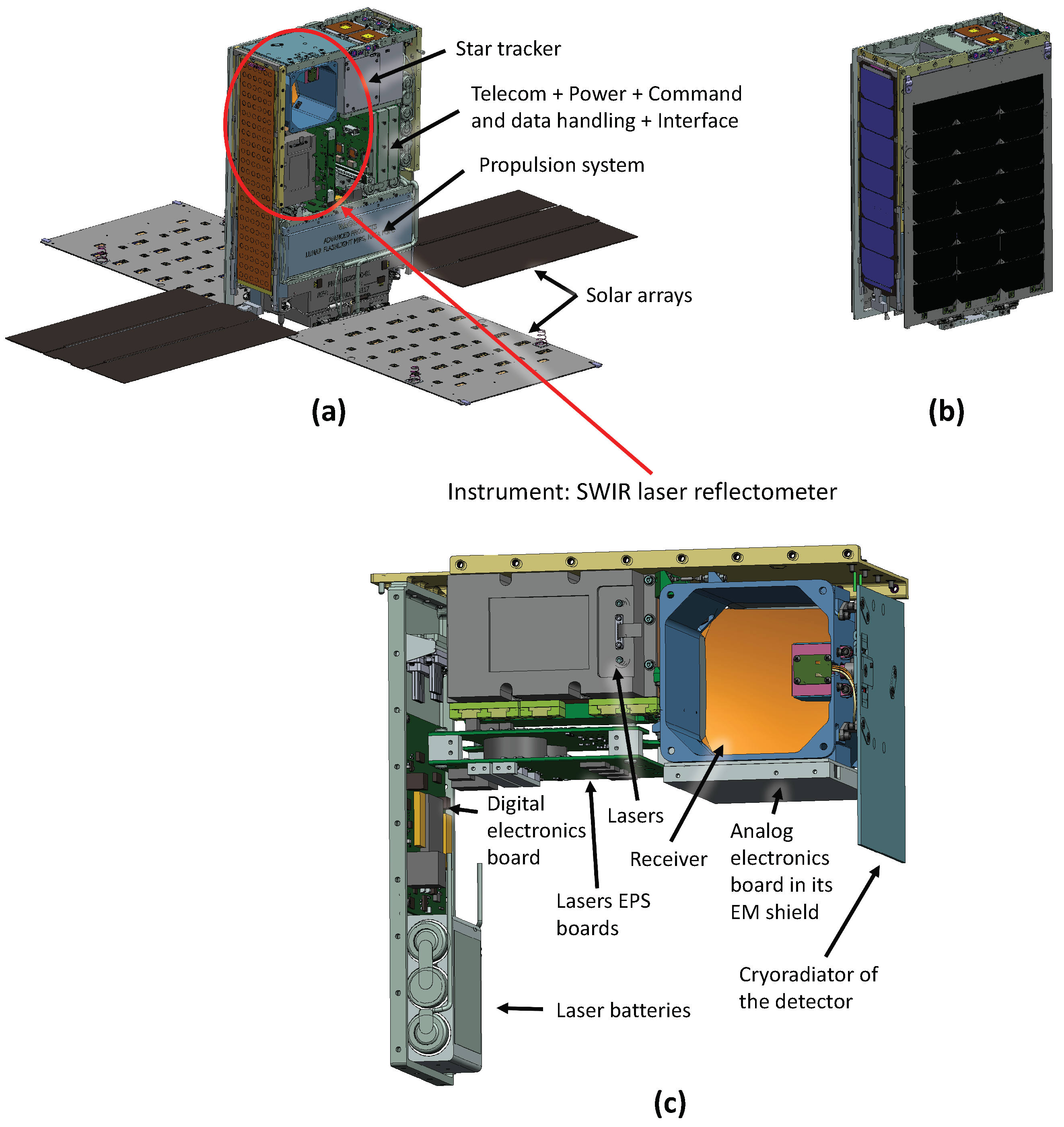
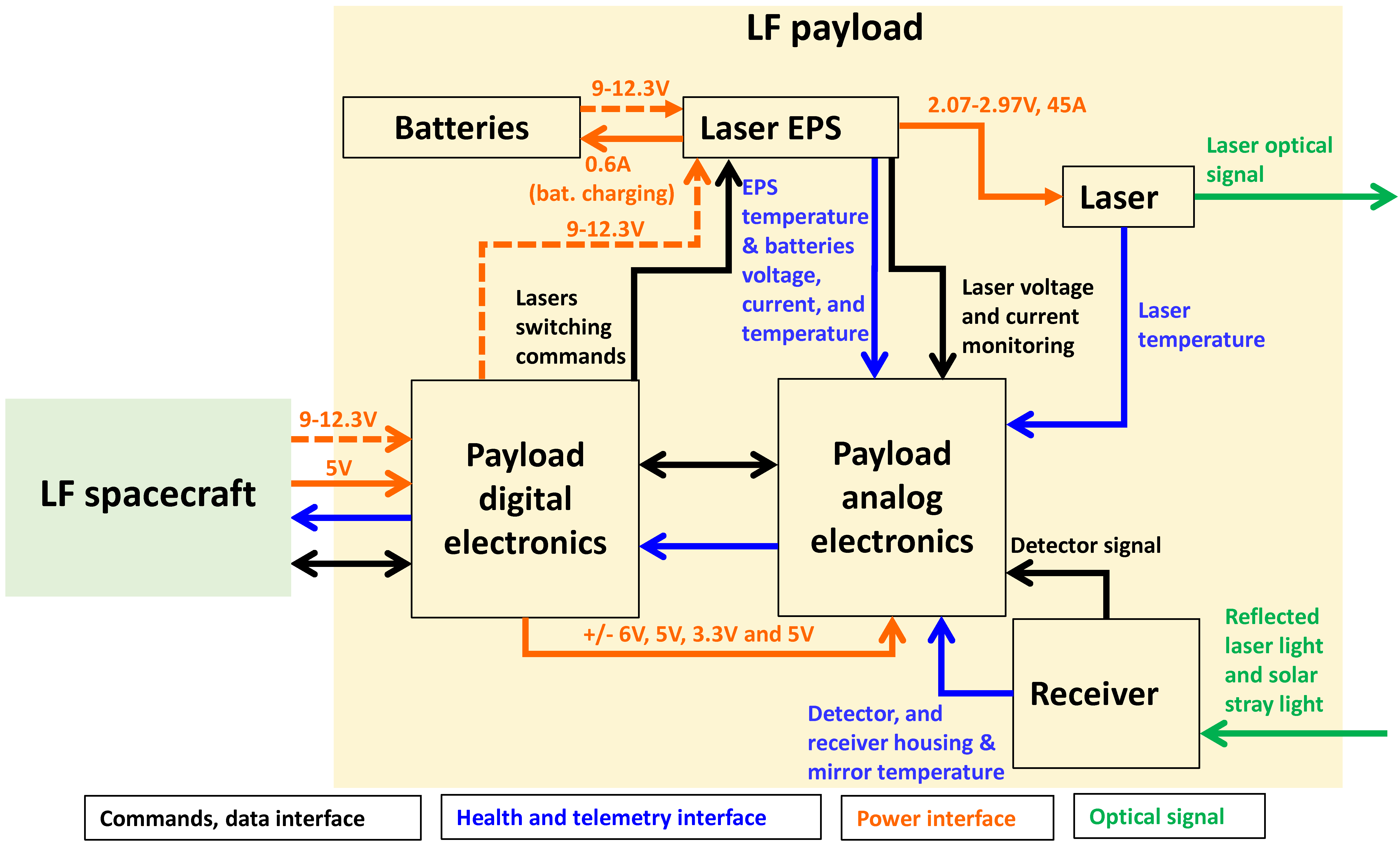
2. Lunar Flashlight CubeSat

The LF CubeSat will inherit the compact form factor of the 6U CubeSat canisterized satellite dispenser standard with some slight modifications to accommodate a maximum mass of 14 kg for a form factor of 116.2 × 239.4 × 366 mm (Tyvak Nano-Satellite Systems Inc. dispenser specifications). As is common with CubeSats, LF will employ commercial off-the-shelf (COTS) components that have been screened for use in space applications, and will have limited fault redundancy. The LF spacecraft propulsion system is a novel technology developed by VACCO Industries, Inc. and will use “green” monopropellant [39]. The transfer of the raw measurements and the remote control of the spacecraft will be achieved by a miniaturized radio called “Iris” [40], which has recently been used by Mars Cube One (MarCO) CubeSats launched to Mars in May 2018. After the ejection of the LF spacecraft from the dispenser, four solar panels deployed in the configuration shown in Figure 1(a) will supply the electrical power to charge the spacecraft batteries. Figure 1(b) illustrates the stowed configuration of the LF spacecraft.

The LF instrument, depicted in Figure 1(c), occupies 2U of the 6U spacecraft. It is a multi-band reflectometer based on an optical receiver that is aligned with four high-power diode lasers (procured from Coherent DILAS Inc.), each emitting in a different wavelength in the SWIR spectral region. These wavelengths, which are obtained by customized epitaxy, correspond to peak absorption for water ice (1.495 µm and 1.99 µm) and the nearby continuum (1.064 µm and 1.85 µm). The diode lasers are pumped at 45 A with voltage ranging from ~2.07 V to ~2.97 V (~2.97 V at 1.064 µm, ~2.07 V at 1.495 µm, and ~2.9 V at 1.85 µm and 1.99 µm), which is supplied by the laser electrical power system (EPS) board and laser Lithium ion (Li-ion) batteries. The laser optical powers (peak powers) at 45-A pump current are as follows: ~73 W at 1.064 µm, ~30W at 1.495 µm, and ~15 W at 1.85 µm and 1.99 µm. In order to dissipate the thermal power from the lasers, the laser module is thermally coupled to a phase-change material (PCM). More than 99% of the emitted optical energy by each of the lasers is encircled within a full angle of 17 mrad. The receiver is based on an off-axis bare aluminum paraboloidal mirror that collects the incoming light onto a single-pixel indium gallium arsenide (InGaAs) detector with a 2-mm diameter, and has been designed to obtain a uniform 20-mrad field of view (FOV). In order to cool the InGaAs detector down to 208 K during science data passes, the instrument uses a cryoradiator that is thermally coupled to the detector and stabilized by a proportional–integral–derivative (PID) regulator controlling a heater mounted on the cryoradiator. An analog electronic board reads and amplifies the detector output current. This signal is then digitized at 100 kHz by the digital electronics board. A block diagram of the instrument is given in Figure 2.

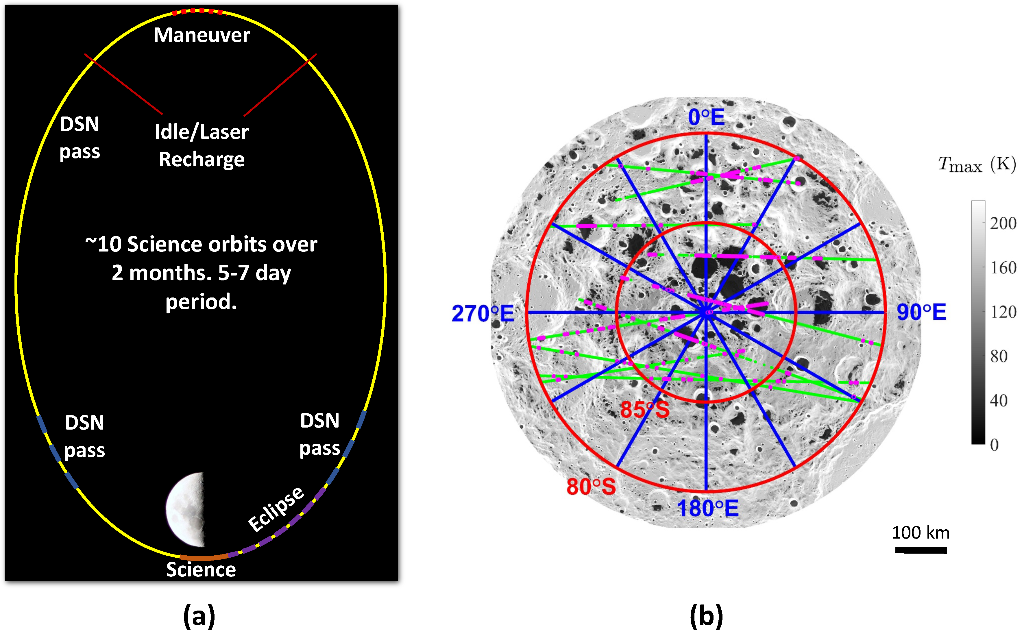
3. Lunar Flashlight Mission

3.1. Measurement Goals

The measurement goal of Lunar Flashlight is to identify locations where water ice is present at the surface of the Moon as a frost. To accomplish this goal, the spacecraft will measure surface reflectance band ratios with a spatial resolution of 10 km or better with multiple measurements in permanently shadowed and occasionally sunlit regions poleward of 80° S latitude. The payload is designed to measure the surface abundance of water ice with concentrations of 5 wt% or less, down to as little as 0.5 wt%. This percentage of water ice concentration (0.5 wt%) corresponds to the minimum quantity that has been defined as useful for in situ resource utilization [5]. As depicted in Figure 3, two of the four wavelengths (~1.495 µm and ~1.990 µm) correspond to overtone vibrational absorption features for water ice, while the two other wavelengths (~1.064 µm and ~1.850 µm) correspond to nearby continua. The measurements will ratio the reflectance value in the absorption features to the continuum in order to determine the water ice abundance.

Previous investigations have revealed evidence for ice at the lunar poles, but have been unable to determine its form or quantify its abundance with a high degree of certainty. For example, the Lyman-α Mapping Project (LAMP) instrument onboard the Lunar Reconnaissance Orbiter (LRO) detected the presence of ~1 wt% to 10 wt% of water within most South polar cold traps, but these data could not uniquely distinguish water ice from adsorbed H₂O or OH molecules [4]. The Lunar Crater Observation and Sensing Satellite (LCROSS) mission detected water ice at concentrations of ~5–7 wt%, but only at one location [20]. LOLA reflectance measurements detected bright regions within the cold traps at both poles, but only used a single 1064-nm wavelength [29]. More recently, H₂O ice detections have been made using scattered light with the Moon Mineralogy Mapper, but these data are intrinsically very noisy, and cannot be used to determine ice abundance at any given location [27]. New measurements are needed in order to uniquely identify and map water ice at the Moon’s poles at operationally useful scales.

3.2. Mission Design

LF will be placed in near-rectilinear orbit around the Moon for two months. The instrument will target PSRs from altitudes of 12.6 to 52.4 km within 10° of latitude from the lunar South Pole from 10 of the orbits; see Figure 4a. Figure 4b shows the achievable PSR coverage map based on the available spacecraft propulsion resources.

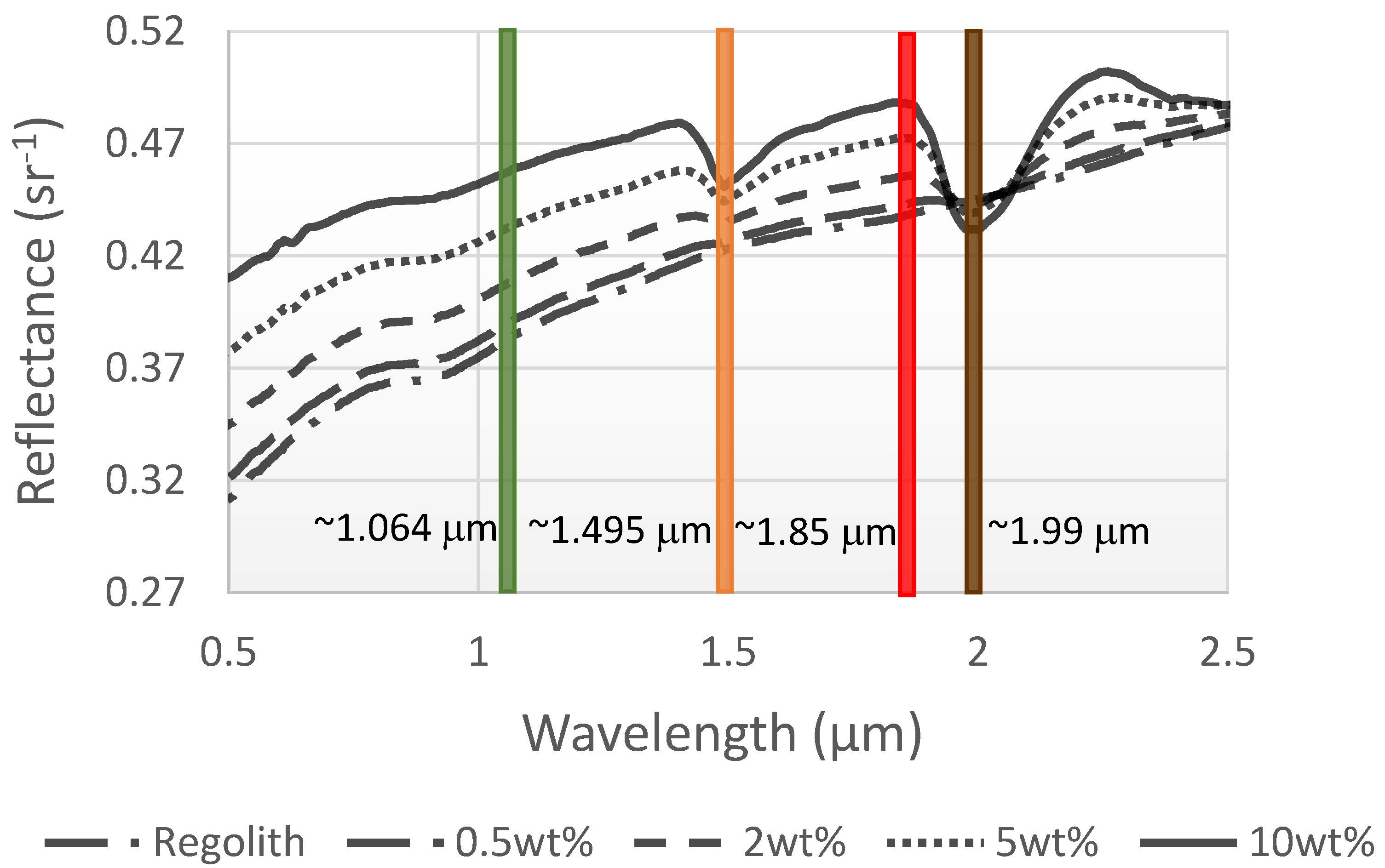
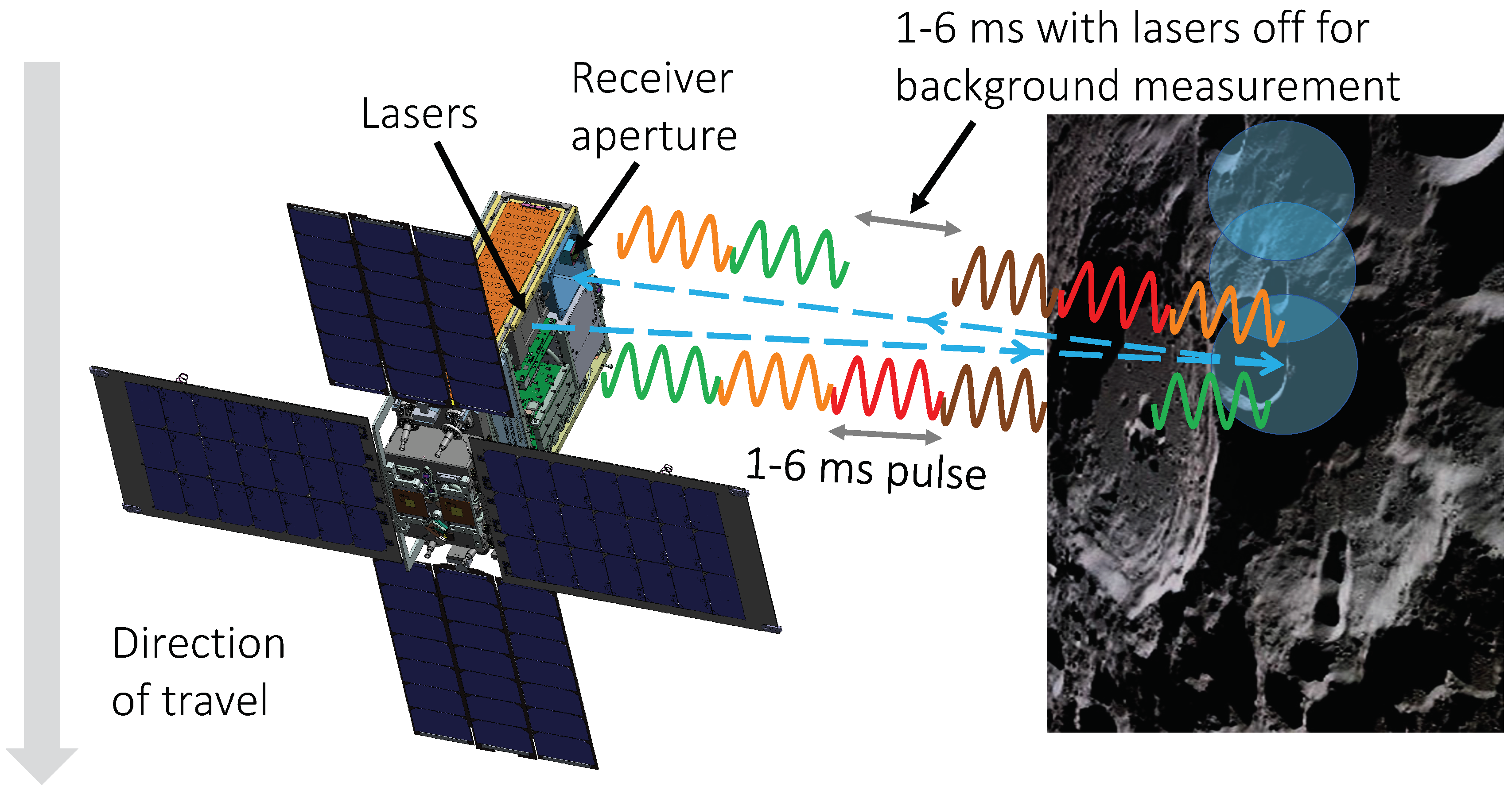
3.3. Principle of Operation

The lasers fire sequentially with a pulse width of 1 to 6 ms each (6 ms nominally), followed by a pause of 1 to 6 ms (6 ms nominally) with all of the lasers off to measure the background. The flight electronics have been designed to be able to change the laser pulse width and the firing sequence. The goal is to be able to take more than one dark frame measurement per laser firing sequence during science data paths in case of unexpected background fluctuations. The optical receiver measures a portion of the light reflected from the lunar surface within its solid angle. The background consists of the sum of the detector dark current, the detected thermal emission of the receiver, and the detected solar illumination reflected from the lunar surface to the receiver inside and outside of its FOV. Theoretically, there will not be any dark current, because the detector is operated at zero bias. However, dark current can be present in the case of a small parasitic bias introduced by the electronics reading the detector. The instrument background is subtracted in post-processing from the measured signals. In order to improve the signal-to-noise ratio (SNR), for each spectral band, the measurements are averaged over the time in which the laser-illuminated area on the lunar surface moves a distance corresponding to the desired mapping resolution of water ice (10 km or less). As a result, Lunar Flashlight will actually measure the average water ice concentration over distances a maximum of 10 km long. The laser spot speed on the Moon surface during science data paths varies from 2.22 to 2.33 km/sec. Considering an average laser spot speed of 2.28 km/sec, a mapping resolution of 1 km corresponds to 1/2.28=0.44 second of integration time, and a mapping resolution of 10 km corresponds to 10/2.28=4.4 seconds of integration time. From the measurements of the reflected laser light in each of the four spectral bands, the continuum/absorption reflectance band ratios are then calculated and analyzed to derive the water ice content within the illuminated area by the lasers. During the planned two-month primary mission, LF will pulse the lasers for a maximum time of 2 to 3 minutes per orbit (due to the thermal dissipation constraints of the instrument) toward the PSRs and occasionally sunlit regions (when in eclipse during the measurements) of the lunar South Pole (see Figure 4). The instrument operation concept is depicted in Figure 5.

Note that LF chose a design using temporal multiplexing and a common receiver for all of the spectral channels instead of a simultaneous acquisition on four spectrally filtered detectors. Given the very demanding mass and volume resources of a CubeSat mission, this payload design is the result of a challenging system engineering effort that maximizes the overall instrument SNR while allowing a simple receiver optical design.

3.4. Algorithm to Derive Water Ice Content from the Instrument Signals and Instrument SNR Impact on Science Measurements

The detector current I_d,λ that is due to the detected laser light emitted at a wavelength λ and reflected from the lunar surface is equal to:

$$I_{d,\lambda }=\frac{P_{\lambda }\left(T_{laser},I_{laser}\right)\times {\alpha }_{\lambda }\left(W\right)\times \Gamma \times R_{\lambda }\times {{\displaystyle \int }}^{}{\mathrm{PST}}_{\lambda }\left({\theta }_x-{\mathsf{\delta }}_x,{\theta }_z-{\mathsf{\delta }}_z\right){\mathrm{LDP}}_{\lambda }\left({\theta }_x,{\theta }_z\right)\mathrm{d}{\theta }_{x}d{\theta }_z}{A^2},$$

(1)

where R_λ is the responsivity of the detector at λ, P_λ is the emitted optical power by the laser at λ that depends on the temperature T_laser of the laser and the pump current I_laser, α_λ is the regolith normal reflectance at zero-phase angle at λ for a given water ice content W, $\Gamma$ is the receiver aperture area, δ_x and δ_z are the misalignment angles between the lasers and the receiver, PST_λ(θ_x,θ_z) is the receiver point source transmittance function at λ, LDP_λ(θ_x,θ_z) is the laser divergence profile normalized by the integrated radiance over θ_x and θ_z for the laser emitting at λ, and A is the altitude of the spacecraft above the lunar surface. The PST represents the fraction of the photons at the receiver aperture that is detected by the receiver detector as a function of the incident angles θ_x and θ_z, and LPD is the distribution of the optical energy emitted by the laser as a function of the divergence angles θ_x and θ_z (see Section 4 for more details). The integral in Equation (1) is the detected fraction of the laser light reflected from the lunar surface to the receiver aperture, and $\Gamma /A^2$ is the solid angle subtended by the receiver aperture. For the sake of simplicity and given the narrow divergence of the lasers (see Figure 6), α_λ has been moved out of the integral in Equation (1). This approximation has an insignificant impact on the results that follow.

The two reflectance band ratios ${\alpha }_{\lambda \_continuuum}/{\alpha }_{\lambda \_peak}$ are measured as follows:

$$\frac{{\alpha }_{\lambda \_continuuum}}{{\alpha }_{\lambda \_peak}}=\frac{I_{d,\lambda \_continuuum}\times C_{\lambda \_peak}\left(T_{laser,\lambda \_peak}, I_{laser,\lambda \_peak}\right)}{I_{d,\lambda \_peak}\times C_{\lambda \_continuum}\left(T_{laser,\lambda \_continuum},I_{laser,\lambda \_continuum}\right)},$$

(2)

where C_λ are the calibration functions that are obtained through an end-to-end test of the instrument. During the instrument calibration, ${\alpha }_{\lambda \_continuuum}/{\alpha }_{\lambda \_peak}$ is known because it corresponds to the calibrated values of standards illuminated by the LF instrument, and $I_{d,\lambda \_continuuum}$/$I_{d,\lambda \_peak}$ is measured to calculate $C_{\lambda \_peak}/C_{\lambda \_continuum}$ at different laser temperatures and pump currents (T_Laser and I_laser are monitored by the LF payload, see Figure 2). The calibration functions C_λ also depend on R_λ and on the integral in Equation (1), but these values are fixed; that is why they are not represented as variables in the C_λ functions that are used in Equation (2) (I_laser should also be a constant, as it is stabilized by the instrument, but calibration functions will also be measured as a function of I_laser in case of unexpected fluctuations during the mission). Note that because LF only measures ratios of reflectance, no absolute calibration of the instrument is needed, which greatly simplifies the calibration.

Based on the data depicted in Figure 3, a W change from 0 wt% to X wt% approximately corresponds to a ${\alpha }_{\lambda \_continuuum}/{\alpha }_{\lambda \_peak}$ change of 2X % in the region 0 wt% to 3 wt% for the reflectance band ratio using the two longest wavelengths, and to a ${\alpha }_{\lambda \_continuuum}/{\alpha }_{\lambda \_peak}$ change of 1.5X % for the reflectance band ratio using the two shortest wavelengths. Thus, in order to discriminate W=0 wt% from W=X wt% at n-sigma confidence level (meaning that the error bars on the two measurements cannot overlap), the minimum $SN{R}_{Xwt\%,n\sigma }$ required on the measured ${\alpha }_{\lambda \_continuuum}/{\alpha }_{\lambda \_peak}$ is given by:

$$SN{R}_{Xwt\%,n\sigma }=\frac{200\times n}{X\times \kappa },$$

(3)

where $\kappa$=2 for the two longest wavelengths, and $\kappa$=1.5 for the two shortest wavelengths. Note that Equation (3) gives a necessary condition on the SNR, but not a sufficient one. For instance, the standard deviation on the measurements can be impacted by a non-uniform distribution of water ice within the mapping resolution, which would increase the uncertainty on ${\alpha }_{\lambda \_continuuum}/{\alpha }_{\lambda \_peak}$ and on the averaged water ice content measurements.

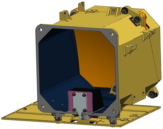
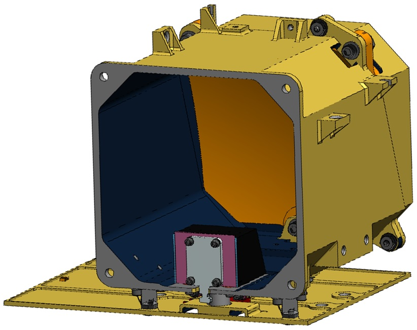
4. Receiver Optomechanical Design

4.1. Receiver Optical Design

This subsection describes the final optical design of the LF receiver completed by Photon Engineering Inc. using the FRED software package, with updated information compared to that given in Vinckier et al. [41]. Given the volume and mass constraints of a CubeSat, the receiver design is constrained to be as simple as possible. The optical system consists in a 70 × 70-mm off-axis aluminum paraboloidal mirror with a single-pixel detector located at the focal position of the mirror. The LF receiver’s InGaAs detector is not sensitive to the total ionizing dose (TID), but it is mainly sensitive to displacement damages. No detector radiation test was performed. However, the LF mission will only last approximately eight months (six months to go to the Moon, and two months of operation), and the probability of having any issue related to displacement damages is insignificant. The receiver occupies 1U of volume (approximately 10 × 10 × 10 cm) out of the 2U of volume allocated to the instrument.

We define the receiver FOV as the incident angle range within which the detection efficiency is maximal and sufficiently uniform (<3.7% non-uniformity within 100% of the FOV; <1.3% non-uniformity within 95% of the FOV). The divergence profiles of the laser beams drive the requirements for the receiver FOV. In the LF laser module design, greater than 99% of the emitted energy is encircled within a full-angle of 17 mrad. The measured far-field normalized laser divergence profiles are depicted in Figure 6.

The receiver FOV has to be large enough to cover the divergence profile of the lasers, and some margins are necessary to accommodate the alignment budget between the lasers and the receiver. However, the FOV cannot be too large in order to minimize the detected solar stray light that would saturate the detector electronics [34]. We designed the receiver to provide a uniform FOV of 20 mrad. Since the focal ratio of the LF receiver is very fast (f <100 mm due to volume constraints), the optical system suffers from large aberrations. Thus, the well-known paraxial approximation given by Equation (4) to calculate the theoretical FOV is no longer valid to accurately estimate the required focal length and detector diameter to provide the 20-mrad FOV.

$$FOV=2\times atan\left(\frac{D}{2f}\right),$$

(4)

where D is the diameter of the detector, and f is the effective focal length of the mirror. However, Equation (4) is still useful to show how to increase/decrease the FOV by modifying the mirror focal length and the detector diameter. We used the ray-tracing software FRED to evaluate the required detector diameter and focal length. The detector diameter was selected from those available off-the-shelf from Teledyne Judson Technologies: 0.25 mm, 0.5 mm, 1 mm, 2 mm, and 3 mm. In order to minimize the noise generated by the detecting chain, which constitutes the main contribution in the instrument error budget [34], the detector diameter must be as small as possible. Ray-tracing simulations showed that a minimum diameter of 2 mm was necessary to obtain a uniform FOV of 20 mrad for this volume-constrained optical design. The resulting optimal focal length is 70 mm.

The optical design has also been optimized for solar stray light rejection. Solar stray light is the sunlight reflected from the lunar surface toward the instrument and scattered onto the detector active area from outside the receiver FOV. Such a situation is depicted in Figure 7.

The stray light scattering model of the FRED software uses the Harvey–Shack surface scatter theory [46]. We performed the simulations considering all of the internal surfaces painted in black, with a mirror roughness set to 30 Å and a cleanliness level equal to CL600 [47].

In order to estimate the LF science performance based on the predicted orbits and lunar surface illumination [34], our model uses the receiver point source transmittance (PST) function calculated in FRED. The PST function represents the receiver detection efficiency as a function of the θ_x and θ_z incident field angles, where θ_x and θ_z are respectively the rotation angles around axis X and Z. The XZ plane is perpendicular to the receiver optical axis. We define the receiver detection efficiency as the fraction of the photon flux passing through the receiver aperture that reaches the detector active area. The optimal vane configuration obtained with FRED, which minimizes the PST function outside the receiver FOV, is depicted in Figure 8. Figure 9 shows the rotational average of the simulated PST function corresponding to the final receiver mechanical design presented in Section 4.2. Figure 10 represents the two-dimensional (2D) PST function for small θ_x and θ_z incident angles to illustrate the receiver FOV, as well as the comparison of the uniform 20-mrad receiver FOV with the averaged laser beam divergence profiles.

Table 1. Principal technical specifications of the receiver design. PID: proportional–integral–derivative, RMS: root mean square.

Receiver dimensions	~80 × 80 × 95 mm 1
Receiver aperture	~75 × 75 mm 1
Mirror surface requirements	70 × 70 mm bare aluminum off-axis paraboloidal mirror, post-polished Focal length: 70 mm Surface flatness: 2λ at 632.8 nm RMS roughness: 30 Å
Science detector	2.4-µm cutoff InGaAs Teledyne Judson with a 2-mm diameter detector in a C11 package, unbiased Thermally isolated from the receiver structure and cooled at 208 K by a cryoradiator thermally stabilized by a PID regulator and a heater mounted on the cryoradiator Shunt impedance at 208 K: 2 MΩ typical, 1 MΩ min Capacitance at 208 K and 0-V bias: 4 nF typical Noise-equivalent power (NEP) at 2.06 μm, 208 K, 1 kHz, and 0-V bias: 9.3×10−14 W/$\sqrt{Hz}$ max., 6.6×10−14 W/$\sqrt{Hz}$ typical (manufacturer specifications; this does not include the noise from the reading electronics)
Temperature sensors	Model: “DT-670” from Lake Shore Cryotronics, Inc. One is mounted on the back of the receiver mirror, one is mounted next to the science detector (see Figure 13, lower left)
Responsivity requirements	>0.47 A/W at 1064 nm >0.89 A/W at 1495 nm >1.05 A/W at 1850 nm >1.04 A/W at 1990 nm
Dark current requirement	<2 nA (detector dark current at a detector temperature of 208 K and detected thermal emission from the receiver at a temperature of 248 K for the mirror)
Field of view requirement	20 mrad with <3.7% non-uniformity within 100% of the FOV and <1.3% non-uniformity within 95% of the FOV
Boresight alignment requirement	<1 mrad (this corresponds to a maximum laser signal loss <0.35% based on the measured laser divergence profiles depicted in Figure 6, which is insignificant)

¹ See Figure 16 for more details.

lists the principal technical specifications of the receiver design.

The impact of the receiver requirements on the measurement uncertainty can be evaluated by considering an observation on the lunar surface in eclipse with insignificant solar stray light power that is detected, an altitude of the spacecraft of 12.6 km, ${{\displaystyle \int }}^{}{\mathrm{PST}}_{\lambda }\left({\theta }_x-{\mathsf{\delta }}_x,{\theta }_z-{\mathsf{\delta }}_z\right){\mathrm{LDP}}_{\lambda }\left({\theta }_x,{\theta }_z\right)\mathrm{d}{\theta }_{x}d{\theta }_z$ ≈ 0.675 at 1064 nm, with the same overlap between the receiver FOV and the laser divergence profile for each wavelength, a detector reflectivity of 3%, and a mirror reflectivity mentioned in the caption of Figure 9 for each of the wavelengths. In order to perform conservative calculations of the detector signal, we consider reflectance values corresponding to 0 wt% of water ice in the calculations below. Here is the mean value of the detector current for each spectral band based on Equation (1):

• $I_{d,1064\mathrm{nm}}=\frac{73\times 0.384\times {0.075}^2\times 0.47\times \left[\frac{0.675}{0.945\times (1-0.03)}\right]}{{12600}^2}=344 pA$
• $I_{d,1495nm}=\frac{30\times 0.423\times {0.075}^2\times 0.89\times \left[\frac{0.675}{0.945\times (1-0.03)}\right]}{{12600}^2}=295 pA$
• $I_{d,1850nm}=\frac{15\times 0.438\times {0.075}^2\times 1.05\times \left[\frac{0.675}{0.945\times (1-0.03)}\right]}{{12600}^2}=180 pA$
• $I_{d,1990nm}=\frac{15\times 0.445\times {0.075}^2\times 1.04\times \left[\frac{0.675}{0.945\times (1-0.03)}\right]}{{12600}^2}=181 pA$

The responsivity of the flight detector at 2.06 μm and 208 K has been measured by the manufacturer, and is equal to ~1.48 A/W. Based on the noise-equivalent power (NEP) given in Table 1, the current noise on I_d is thus equal to 1.48×6.6×10^-14 ≈10^-13 A/$\sqrt{Hz}$. As mentioned in subsection 3.3, a mapping resolution of 10 km corresponds to a total integration time of ~4.4 sec. Given that the nominal duty cycle of the lasers is equal to 20%, the maximum integration time per spectral channel is actually equal to 0.88 sec. The corresponding Nyquist frequency is equal to 1/(2×0.88)=0.57 Hz. Thus, the root mean square (RMS) noise on the current for each averaged measurement is equal to 10^-13×(0.57)^1/2 =75.5 fA. This noise is applied two times per spectral channel. Indeed, it is present when measuring laser photons, and when measuring the background with all the lasers off. The error propagates during the background subtraction, and the overall noise due to the detector NEP on each spectral channel is equal to 2^1/2×75.5 = 106.8 fA RMS.

The shot noise ${\sigma }_I$ related to the detection of a current I is given by:

$${\sigma }_I=\sqrt{2qI} \left(\frac{A}{\sqrt{Hz}}\right),$$

(5)

where q is the elementary charge equal to 1.6×10^-19 C. So, the shot noise on the maximal detected instrument background given in Table 1 (2 nA) is equal to 19.1 fA RMS. This noise is applied two times per spectral channel, because the background is present on each spectral channel, and then it has to be subtracted afterwards by the measurement performed with all the lasers off, which quantifies the background. Thus, the error propagates during the background subtraction, and the overall noise due to background subtraction is equal to 2^1/2×19.1=27 fA RMS. Here is the calculated shot noise on the detected laser signal:

• At 1064 nm: 7.92 fA RMS
• At 1495 nm: 7.34 fA RMS
• At 1850 nm: 5.73 fA RMS
• At 1990 nm: 5.75 fA RMS

We can now calculate the receiver SNR on each channel:

• $SN{R}_{Id,1064nm}=\frac{344}{\sqrt{{0.1068}^2+{0.027}^2+{0.00792}^2}}=3115$
• $SN{R}_{Id,1495nm}=\frac{295}{\sqrt{{0.1068}^2+{0.027}^2+{0.00734}^2}}=2672$
• $SN{R}_{Id,1850nm}=\frac{180}{\sqrt{{0.1068}^2+{0.027}^2+{0.00573}^2}}=1632$
• $SN{R}_{Id,1990nm}=\frac{181}{\sqrt{{0.1068}^2+{0.027}^2+{0.00575}^2}}=1641$

The receiver SNR on the reflectance band ratio is equal to [(1/3115)² + (1/2672)²]^-1/2=2028 for the shortest wavelength and [(1/1632)² + (1/1641)²]^-1/2=1157 for the longest wavelength. According to Equation (3), using the shortest wavelengths, an SNR of 2028 on the measured reflectance band ratio corresponds to a water ice discrimination level of 0.2 wt% at the 3-sigma confidence level. Using the longest wavelengths, an SNR of 1157 on the measured reflectance band ratio corresponds to a water ice discrimination level of 0.26 wt% at the 3-sigma confidence level. This is the error on the water ice measurements that is allocated to the receiver subsystem by the receiver requirements at the minimal spacecraft altitude of 12.6 km. Of course, for measurements performed at altitudes >12.6 km, the SNRs decrease, and the allocated uncertainties on water ice measurements increase. These numbers have to be compared with the LF requirement on water ice concentration measurements: a water ice detection level of 5 wt% or less at 10-km mapping resolution, implicitly with the 3-sigma confidence level.

The SNRs calculated above are not the ones that are achievable by the instrument, but rather only the ones that are achievable by the receiver subsystem. The scope of these calculations is to quantitatively show the link between the receiver requirements mentioned in Table 1 and the allocated error on the science performance. Although the scope of this paper only focuses on the receiver subsystem, it should be mentioned that the SNR that is realizable by the entire instrument is driven by the noise of the electronics that is used to read the detector, which is not included in the calculations above. The detector electronics is in its final design phase to maximize its performance. No measurement of the detector NEP has been performed; the plan is to measure the noise of the entire ”receiver and electronics” chain through an end-to-end test once the electronics is redesigned.

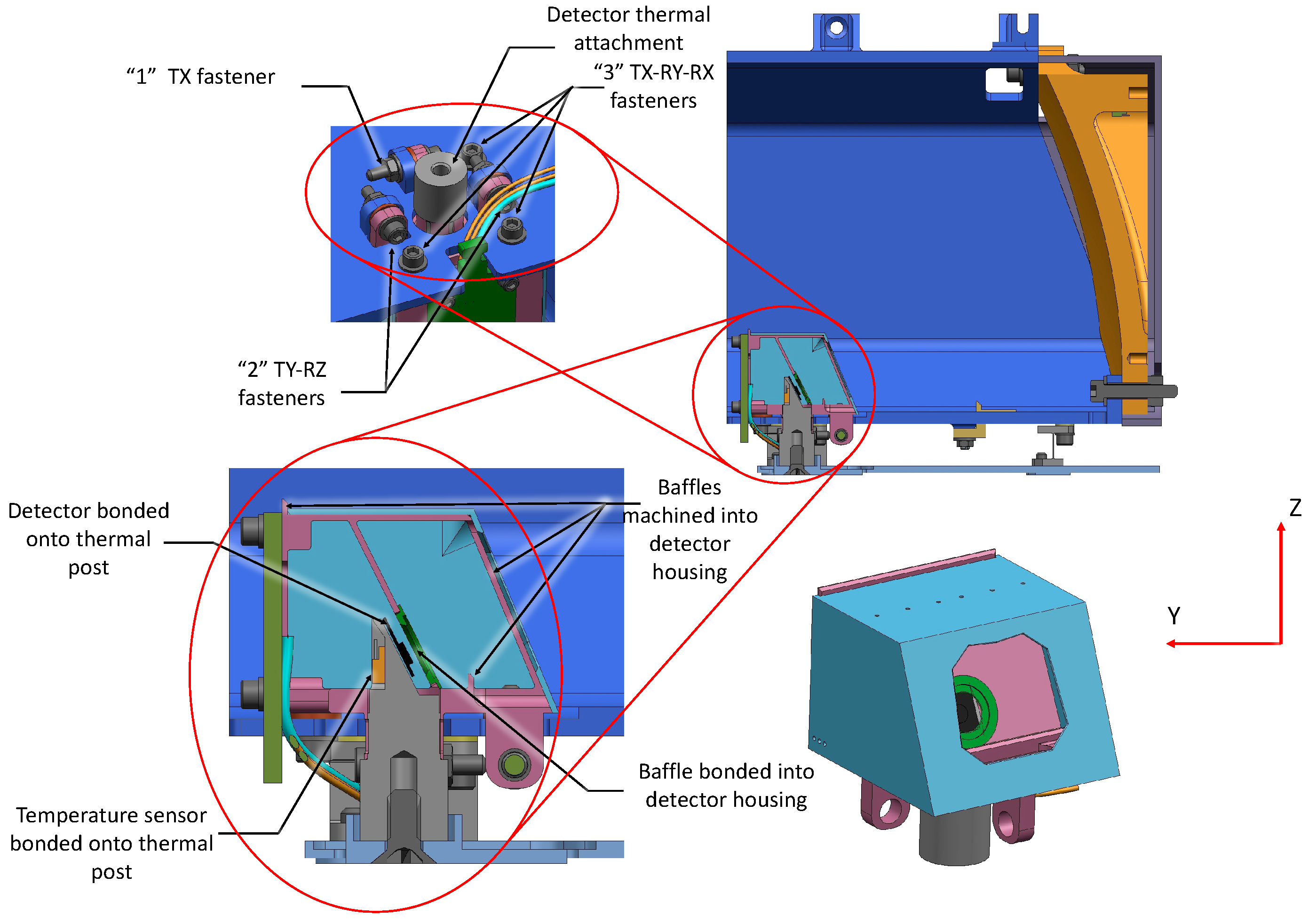
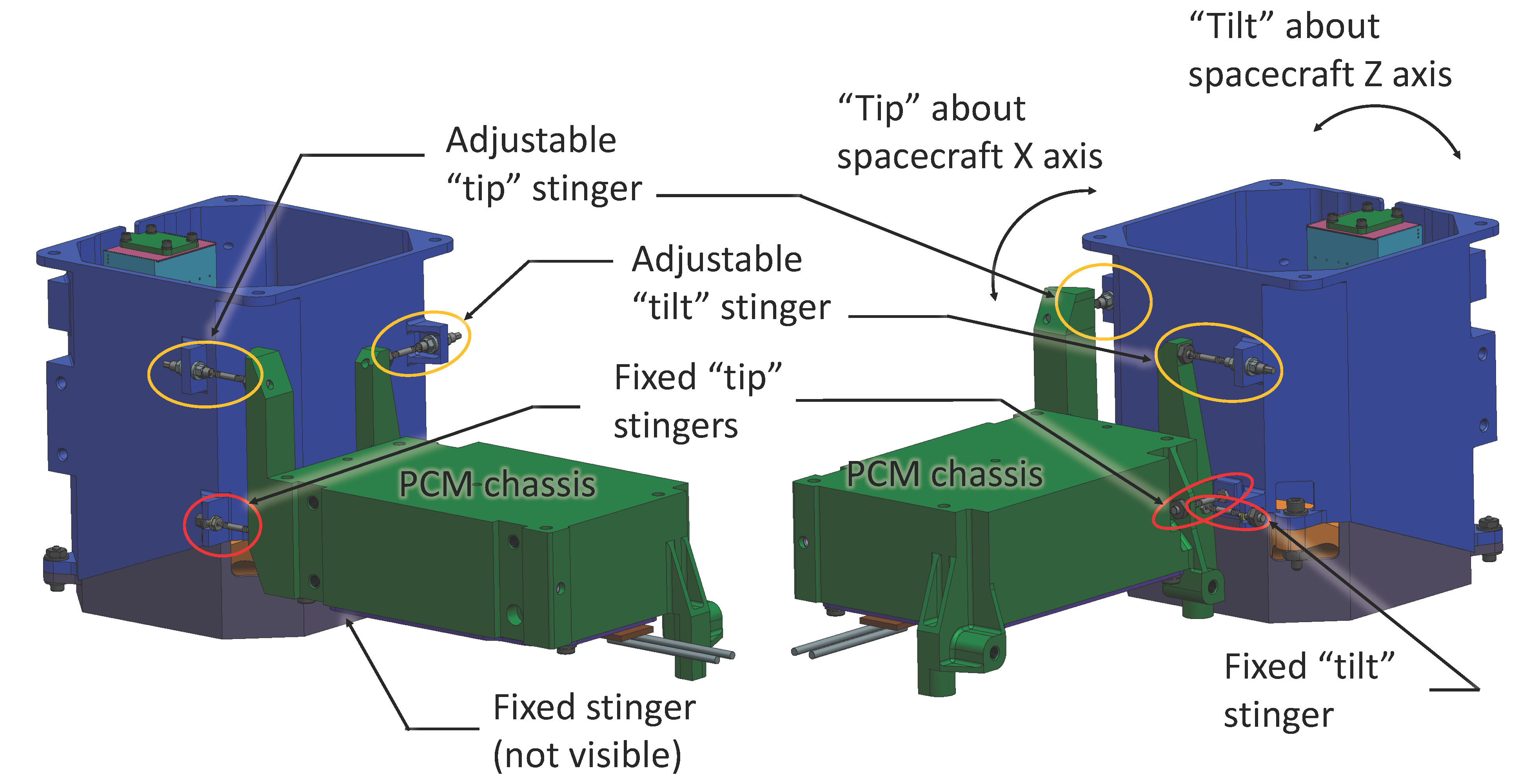
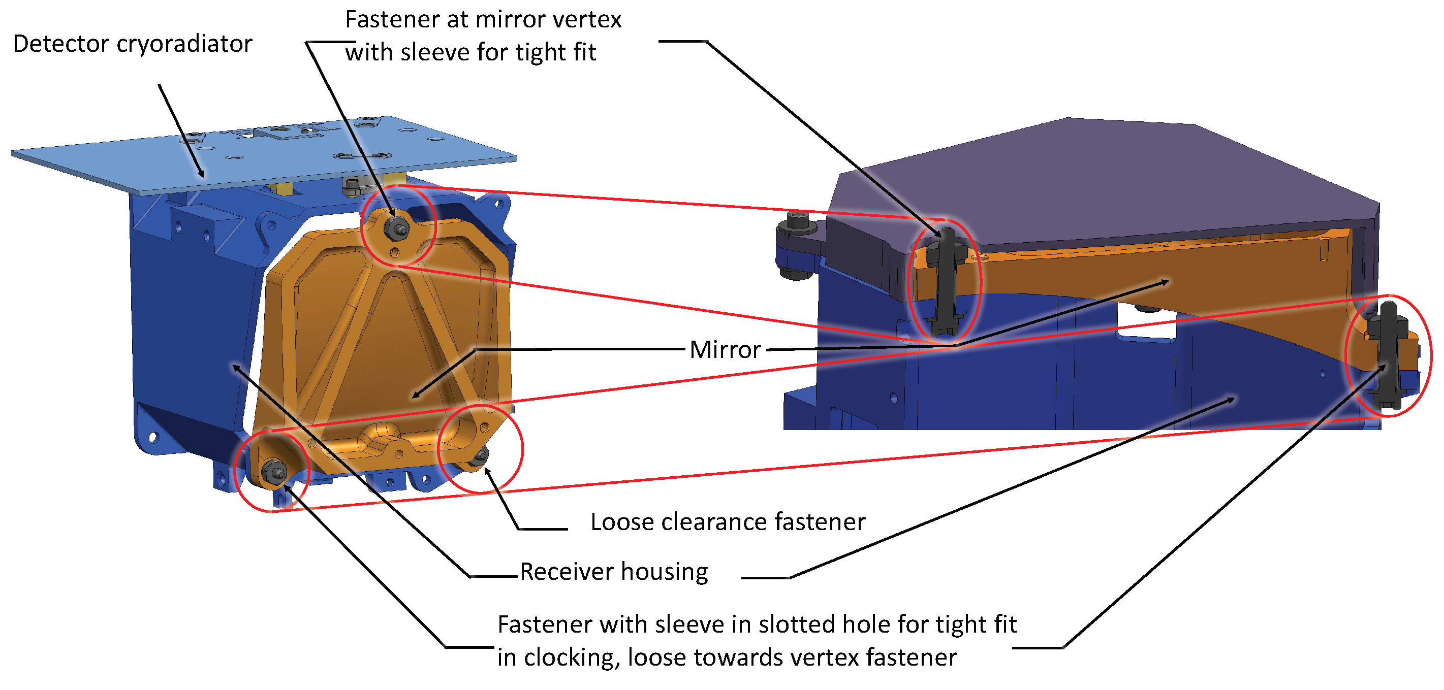
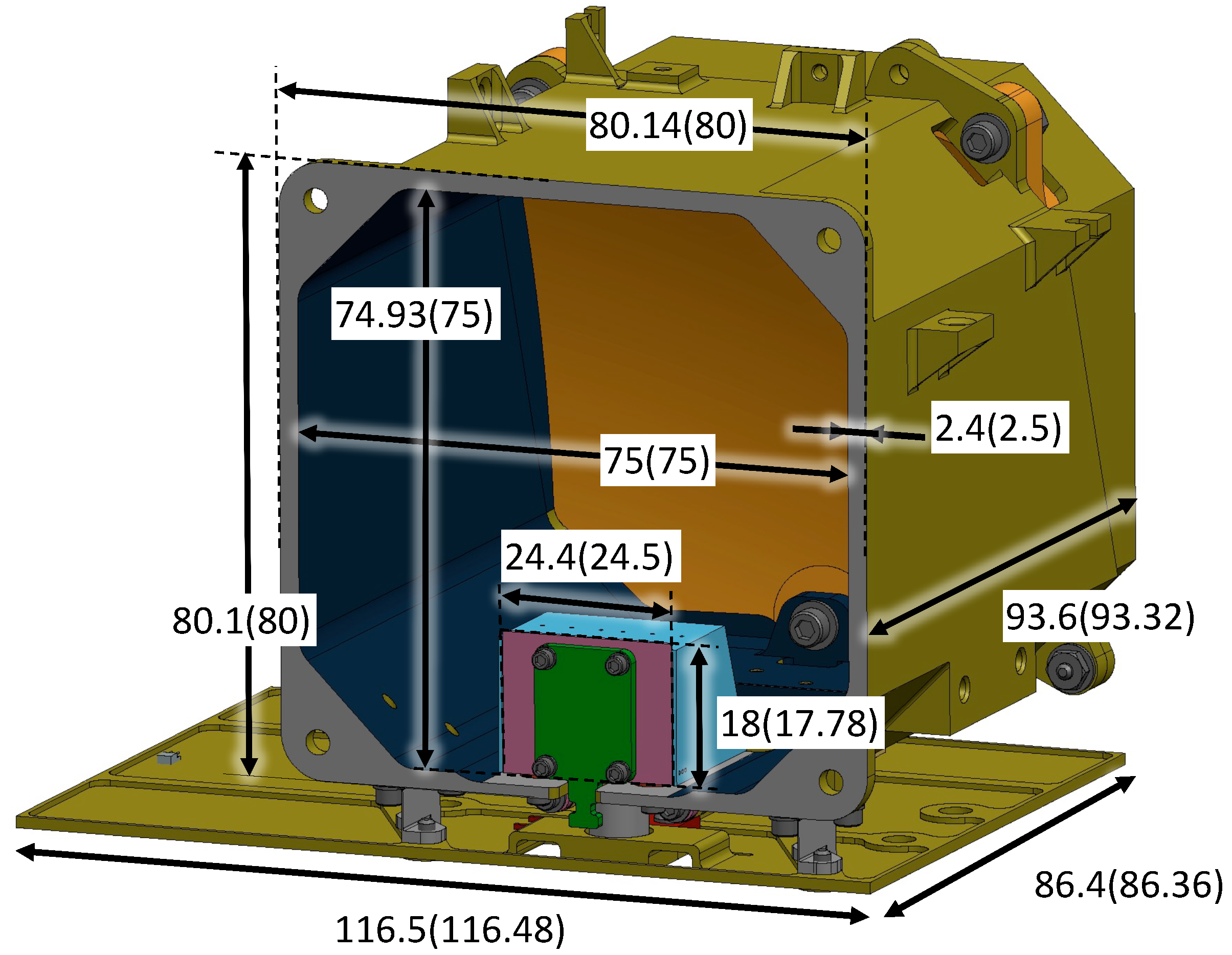
4.2. Receiver Thermal and Mechanical Designs

The optical design defines only the dimensions and the relative positions of the front surface of the mirror, the detector, and the stray light control elements (receiver housing, baffles, vanes). The mechanical and thermal design defines all the remaining dimensions, materials, and processes to support the fabrication of the complete receiver. This subsection describes the final thermal and mechanical designs of the LF receiver created by Sierra Lobo Inc., with updated information compared to the ones given in Vinckier et al. [41].

The LF instrument assembly depicted in Figure 11 includes three subsystems: the laser module, the receiver module, and a part of the LF thermal subsystem. The laser module consists of multiple laser diodes, collimation lenses, and the related electrical and mechanical hardware contained in an enclosure with a copper heatsink, which is bolted to an aluminum-alloy chassis containing the PCM. The PCM module not only dissipates the thermal power emitted by the lasers during operation, but it also forms the mechanical structure to which the receiver module is attached.

The receiver module comprises essentially four major components: an off-axis paraboloidal (OAP) mirror, the receiver housing, a detector subassembly, and a cryoradiator. The OAP is machined from rapidly solidified aluminum (RSA) alloy RSA-6061, using conventional machining for the mirror blank, single-point diamond turning (SPDT) to achieve the surface figure, and post-polishing to reduce surface scatter. Three integral mounting pads on the OAP are cut via SPDT in the same pass as the optical surface to provide a precision datum to the Al alloy 6061-T6 receiver housing. Similarly, the mounting feature that is used to define the axis of the OAP on the SPDT lathe is utilized as a mounting feature to the receiver housing. This design paradigm provides the basis of a “snap-together” optomechanical system (see Figure 12). The intent was to have the mating features placed in a final step using SPDT, although schedule constraints prevented this approach. Instead, the final mounting of the OAP to the conventionally machined housing used an epoxy bed of Stycast 2850FT to mitigate differences in flatness and coplanarity at the faying surface. The radial position of the OAP to the housing was controlled to high precision through a close-fitting sleeve between the aforementioned axial tooling feature on the OAP, and a similar feature on the housing. A secondary sleeve at one of the remaining mounting pads provides a clocking constraint to the housing with a radial slot. OAP to housing athermalization is achieved through use of similar materials. The external surfaces of the receiver housing are electroplated with gold to provide passive cooling.

The third member of the receiver module, the detector subassembly, provides mechanical mounting for the InGaAs detector, stray light baffling, thermal isolation from the receiver housing, and thermal connection to the cryoradiator. Additionally, the electromechanical packaging of the detector and detector temperature sensor are provided by this subassembly. Materials for this subassembly were chosen to be of a similar coefficient of thermal expansion (CTE) to the ceramic detector package. The detector is bonded to a titanium–zirconium–molybdenum (TZM) alloy post. This provides the mechanical and thermal connection to the detector housing and cryoradiator, respectively. This post is, in turn, bonded to a titanium alloy detector housing. The detector housing has mounting features at its base for attachment to the receiver housing with conventional screw fasteners, and precision shims for positioning. They are arranged in a 3–2–1, semi-kinematic configuration with the mounting planes crossing at the intersection of the TZM detector post and the Al alloy receiver housing (see Figure 13). This symmetry affords some degree of athermalization of the detector position through the interface between the receiver housing and detector subassembly CTEs.

The complex aperture shapes and edge profiles of the baffles resulting from the stray light analysis dictated a multiple-piece detector housing. The detector housing base has baffle features, and forms the optomechanical structure for the detector subassembly. It is machined, both conventionally and with wire electrical discharge machining (EDM) to achieve the necessary form and precision. A turned circular baffle with the prescribed internal diameter and edge profile is epoxy bonded into a mating feature in the housing base. Closeout of the detector subassembly is with a cover that has yet another baffle of the correct shape and edge profile using the same techniques as the detector housing base. All of the pieces are painted internally and externally with Aeroglaze Z-306 flat black paint.

The detector is cooled via the cryoradiator machined from Al alloy 6061-T6. It is affixed to the detector post with a single fastener with interface thermal conductivity augmented by wet-mounting with a conductive polymeric: either Stycast 2850FT or Nusil CV 2942. Thermal isolation between the radiator and the receiver housing is provided by three Ti alloy flexures arranged such that their complicate direction is pointed at the detector post. This allows the radiator to contract relative to the rest of the receiver module without affecting the alignment. The CTE of the Ti flexures is similar enough to the TZM detector post to avoid the excessive stress that is normal to the cryoradiator, although flexure cuts in the radiator provide additional compliance.

The receiver and laser modules are mechanically coupled using six titanium-alloy rod flexures (see Figure 14). These “stingers” maintain boresight alignment while also providing thermal isolation between the laser and receiver. Coarse relative pointing adjustment is achieved by differential shimming between seats machined into the receiver housing, the PCM chassis, and the stingers. Fine tip–tilt adjustment is achieved through two of the six stingers, which are fitted with fine screw threads. These are mated to opposing conical seats in the receiver housing with opposing nuts with ogive faces. When micron-level resolution metrology is actively employed during alignment, 0.05-mrad pointing adjustments are achievable.

5. Receiver Characterization

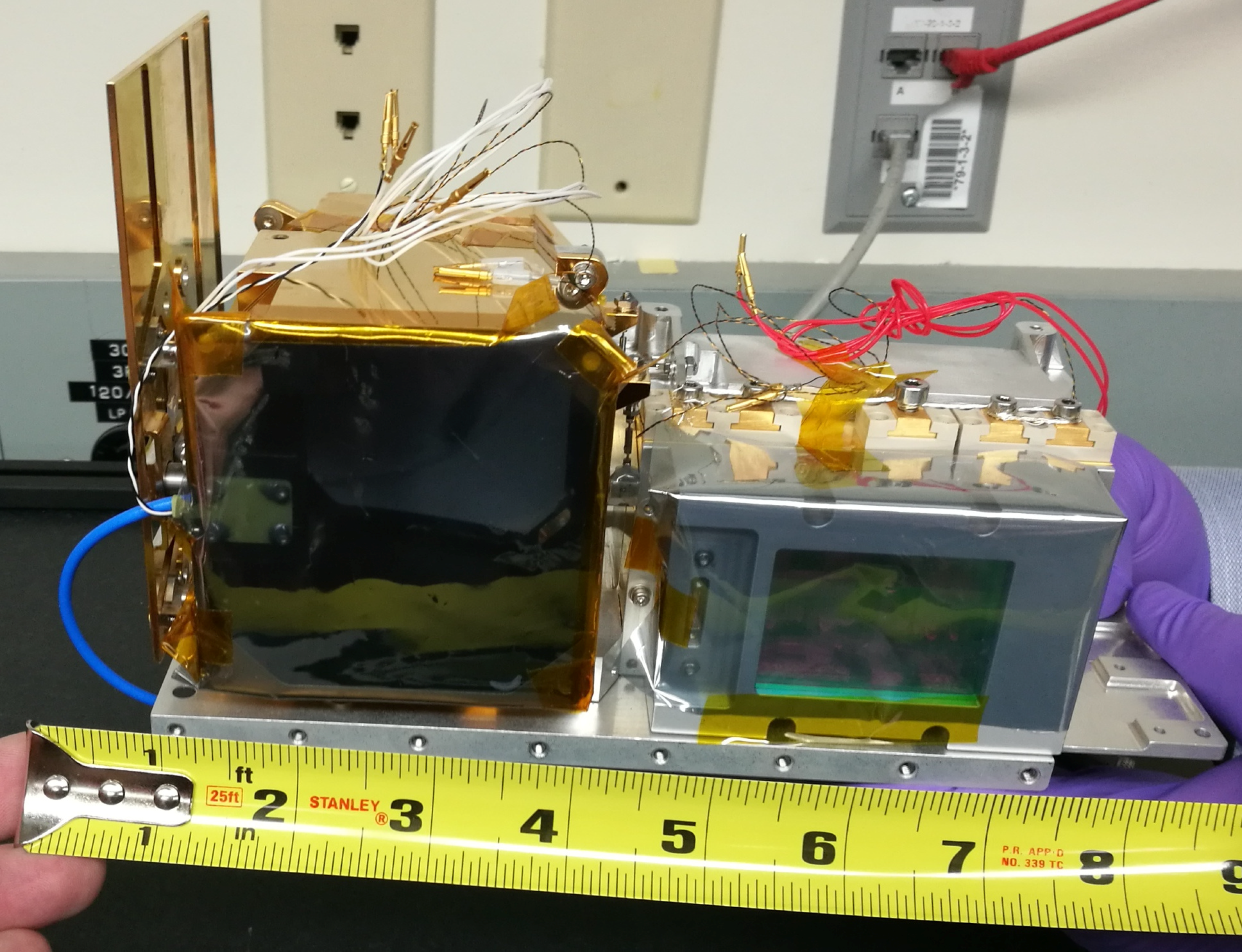
5.1. Flight Hardware Inspection after Delivery to the Jet Propulsion Laboratory

Figure 15 presents the flight LF reflectometer optomechanical assembly. The assembly mass was 1.57 kg, including a ~20 cm ground support equipment (GSE) coaxial cable with its Bayonet Neill–Concelman (BNC) connector. Measurements of the receiver dimensions are presented in Figure 16.

The mirror roughness has been measured to 36 Å on average (15 to 20 Å for most of the surface, except for a band of ~5 mm that hugs the edges of the mirror, which is ~40 Å), and the mirror figure to 1.74 λ at 632.8 nm. This is close enough to the baseline design (see Table 1) to not significantly affect the receiver performance. Indeed, the total integrated scattering (TIS) is roughly proportional to the square of the RMS surface roughness for smooth surfaces (when the RMS surface roughness <<λ) [48]. Thus, increasing the RMS surface from 30 Å to 36 Å would roughly increase the TIS by 44%. A higher TIS means more scattered solar stray light (which increases the shot noise on the measurements) and more scattered laser light (which decreases the detected laser signal). The shot noise related to the detected solar stray light is insignificant in the instrument SNR budget for most of the observations of PSRs and regions in eclipse (see [34]), so the slight increase of the detected solar stray light due to the RMS surface roughness on the instrument SNR can be disregarded. The maximum TIS of the mirror at a surface roughness of 30 Å, corresponding to a wavelength of 1 μm and an incident angle of 0° (we will never experience such an incident angle for the laser light, so the analysis is conservative), is equal to 0.14% according to the database used by FRED; 44% of 0.14% is equal to 0.06%. This very conservative analysis means that increasing the RMS surface from 30 Å to 36 Å would decrease the instrument SNR by less than 0.06%, which is insignificant.

During the integration of the receiver, the internal surfaces of the detector housing shell were left unpainted (see Figure 13, lower right, turquoise part) with Aeroglaze Z-306 black. These surfaces consist of unpolished titanium with BR127 primer applied. FRED simulations have shown that these unpainted surfaces do not lead to any significant degradation of the receiver stray light rejection performance.

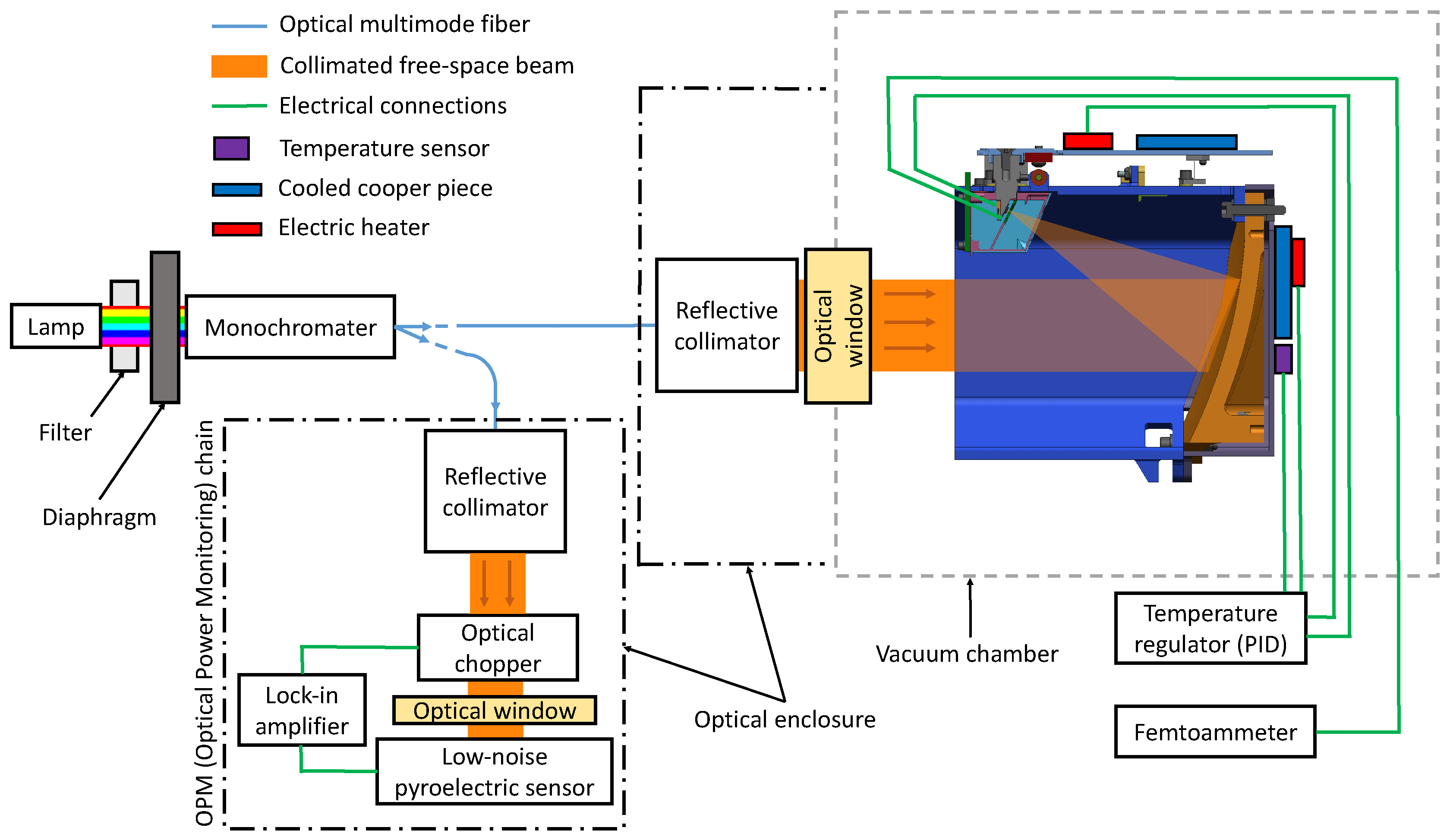
5.2. Spectral Charactarization of the Receiver

We measured the responsivity of the receiver at ± 5% uncertainty (2-sigma confidence level) in the center of the four bands to verify the compliance with the responsivity requirements used in our mission-level performance model. To do so, the receiver housing and the mirror were stabilized at 228 K in a vacuum chamber (pressure: <3×10^-5 torr), while the detector was stabilized at 208 K. The 228 K value corresponds to the middle of the operational temperature range [208, 248] K of the receiver housing and the mirror. The spectral responsivity was also tested at a mirror temperature of 208 K and 248 K, with no noticeable change in measurements.

During operation, the output current of the detector due to detected laser photons will vary from 10 to 344 pA, depending on the wavelength and the altitude for the current proposed lunar orbits. The current range of the flight electronics that is used to read the detector output current is equal to 0 to 10 nA to accommodate for the detected background with margins. The detector is linear up to at least 1 mW of optical power. To spectrally characterize the receiver, the center of the receiver FOV was illuminated through a vacuum chamber optical window with a collimated beam (divergence <1.8 mrad; diameter ~12 mm) of optical power from 160 to 520 nW, depending on the wavelength. In order to maximize the measurement precision and accuracy of the receiver responsivity, the optical output power of the characterization setup has not been attenuated down to the one predicted during the mission. This is not a problem as long as the receiver operates in its linear regime. The light source was a fiber-coupled monochromator aligned with a tungsten lamp, and the other end of the fiber was plugged into a “plug and play” silver-coated reflective collimator. After reading the output current of the detector, the fiber was plugged into another silver-coated reflective collimator to illuminate a low noise (NEP=5 nW/$\sqrt{Hz}$) pyroelectric sensor (diameter of the detector: 5 mm; diameter of the beam on the active surface area: ~4 mm) in order to measure the optical power that was sent to the receiver. An identical optical window to the one used in the vacuum chamber was inserted before the pyroelectric sensor. Both reflective collimators that were used were mounted on a kinematic mount to finely adjust the pointing of the beam. A diaphragm was used to cut off the optical signal emitted by the monochromator to take a dark frame measurement of both the pyroelectric sensor signal and science detector signal. Then, the measurements with the monochromator output light illuminating the receiver mirror were adjusted by subtracting the background. The spectral characterization bench is depicted in Figure 17.

Here is the technical description of the principal components that were used to build the spectral characterization bench depicted in Figure 17:

• 950-nm cut-on wavelength long-pass filter: “FEL0950” from Thorlabs.
• 1450-nm cut-on wavelength long-pass filter: “FEL1450” from Thorlabs.
• Temperature sensors: “DT-670” from Lake Shore Cryotronics, Inc.
• Monochromator: “SDMC1-06G #95 850-2.2u” monochromator from Optometrics aligned with a “TS-20W” tungsten lamp and controlled by a “PCM-02 110V” stepping motor controller (7-nm spectral linewidth, spectral repeatability: ≤0.5 nm).
• Fiber: “FG200LEA” multimode fiber from Thorlabs, 0.22 numerical aperture, Low-OH, Ø 200-µm core, 400 to 2400 nm.
• Reflective collimators: “RC12SMA-P01” and “RC02SMA-P01” protected silver-coated collimator from Thorlabs.
• Pyroelectric sensor: “THZ5B-BL-DZ” from Gentec Inc.
• Digital lock-in amplifier: “T-rad THz module” from Gentec Inc.
• Optical chopper: “SDC-500” from Gentec Inc.
• Femtoammeter: “Keithley 6430” with its remote pre-amplifier; parasitic bias introduced on the detector by the active feedback loop: <1 mV.
• Optical window: “VPW42” 1.5’’ diameter uncoated fused silica optical window from Thorlabs; parallelism: ≤5 arcsec, transmitted wavefront distortion: λ/8 at 633 nm.
• The monochromator was spectrally calibrated (spectral linewidth and wavelength as a function of stepper motor position, repeatability characterization) using the two different optical spectrum analyzers: “HP 70950A” for the 1064-nm and 1495-nm wavelengths, and “Yokogawa AQ6376” for the 1850-nm and 1990-nm wavelengths.

The required and measured responsivity in the center of the four operational wavelength bands are available in

Table 2. Characterization of the receiver responsivity.

Wavelength (nm)	Responsivity measurement (A/W) 1	Responsivity requirement (A/W)
1064	0.51	>0.47
1495	1.06	>0.89
1850	1.36	>1.05
1990	1.37	>1.04

¹ Uncertainty: ± 5%, 2-sigma confidence level. The integration time of the femtoammeter and pyroelectric sensor was set to almost cancel the noise on the measurements (standard deviation on responsivity measurements <0.1%). The uncertainty on the measured responsivity comes from the calibration uncertainty of the equipment.

. As shown in Table 2, all of the measurements meet the requirements. Photographs of the flight hardware inside the vacuum chamber are shown in Figure 18.

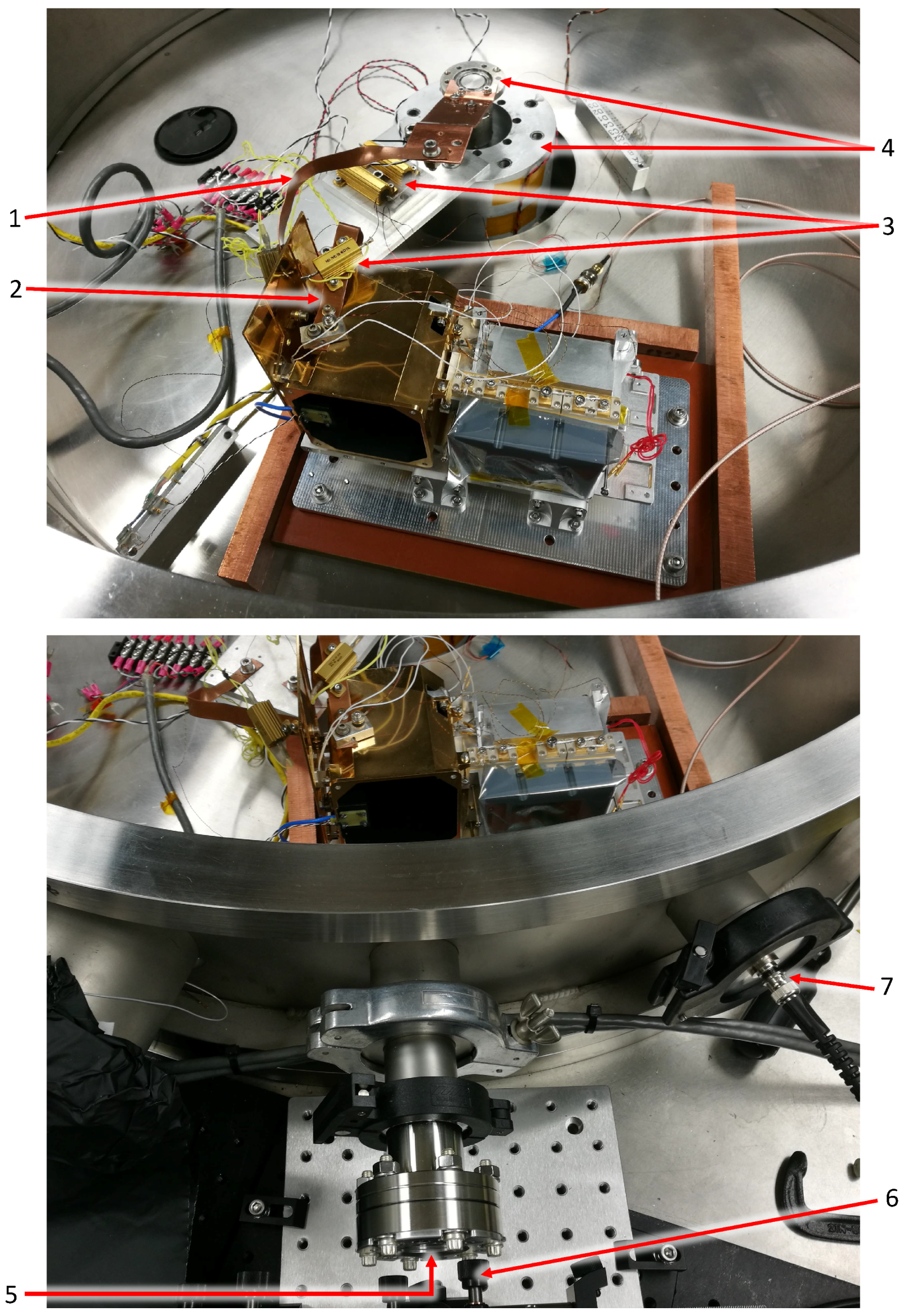
5.3. Characterization of the Dark Current and Detected Thermal Emission

While the receiver was in the vacuum chamber, the output current was measured with the diaphragm closed (see Figure 17). This current is the sum of the detector dark current and the detected receiver thermal emission. A dark measurement of the current was taken with the receiver housing and mirror stabilized at 248 K, corresponding to the highest temperature during operation. If the detector is perfectly unbiased, the dark current of the detector should be null. However, the active feedback loop of the femtoammeter slightly biases the detector (bias <1 mV), which explains why a measurement of dark current in addition to the detected receiver thermal emission is necessary. The requirement was to measure a current <2 nA. A measurement of 0.38 nA was acquired, with an integration time set to get a standard deviation <1%. The goal of this measurement was to ensure that the receiver signal with no incoming light was below the requirement to prevent saturation of the electronics (the requirement for this dark measurement is <2 nA, and the current range of the flight electronics is 0 to 10 nA, so the requirement has been met with a large margin).

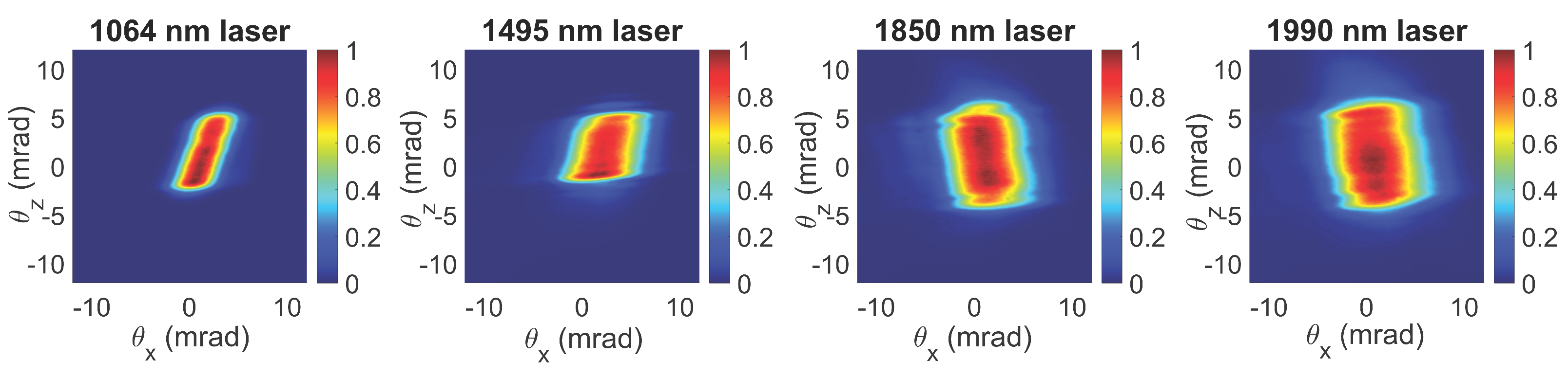
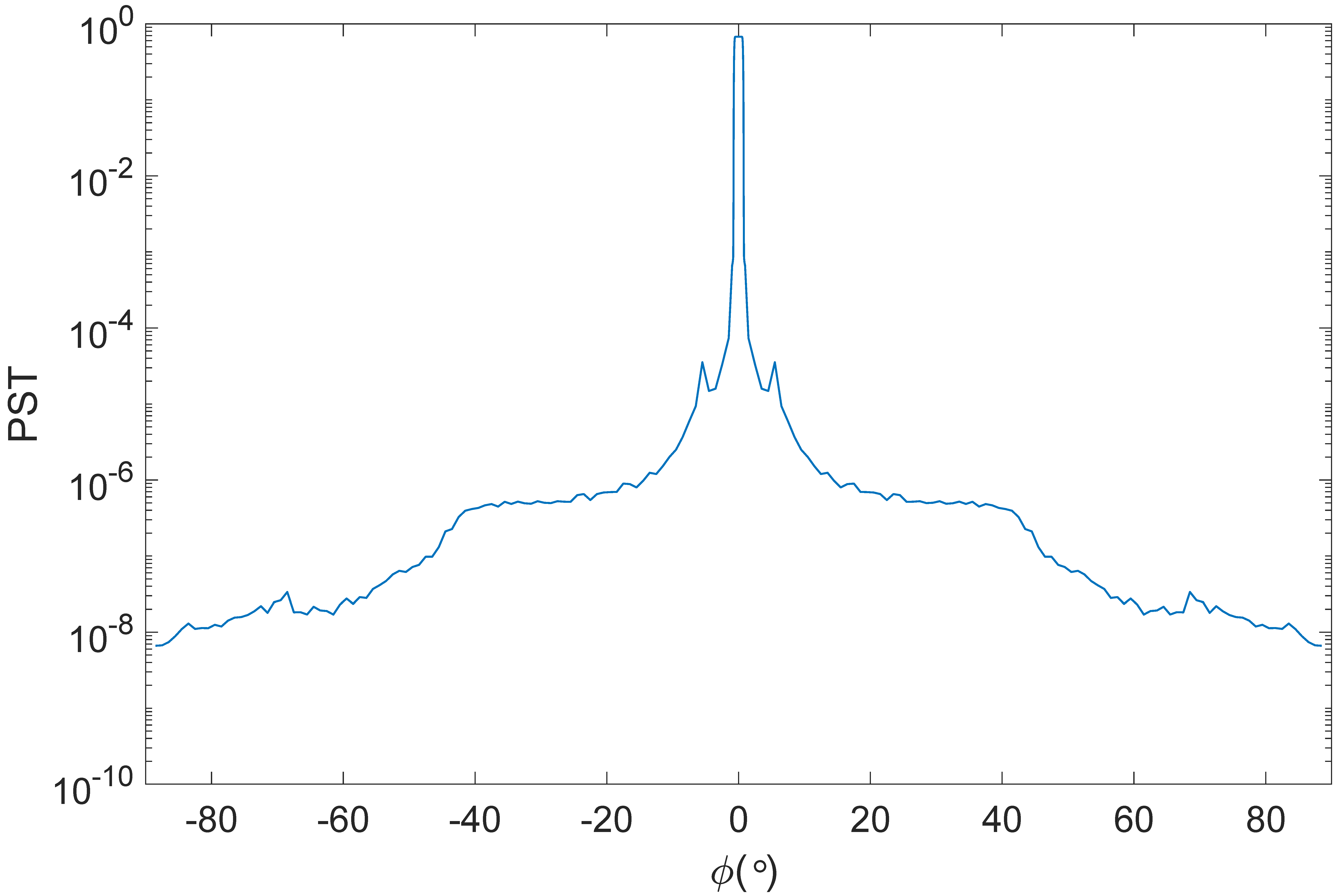
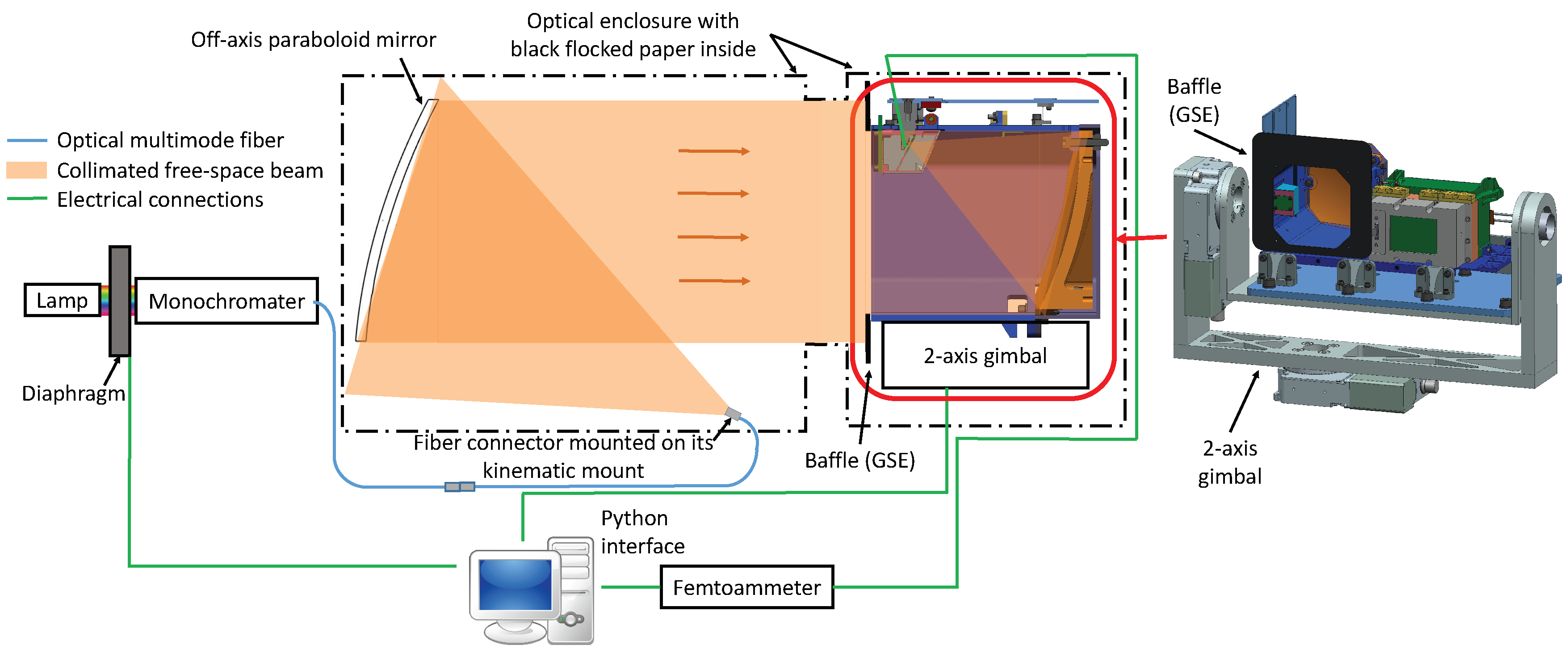
5.4. Charactarization of the Receiver Field of View

The receiver FOV was characterized at room temperature using a motorized two-axis gimbal. The thermal design guarantees a negligible FOV difference between room temperature and the operational temperature. A collimated beam (full-angle divergence <0.35 mrad) illuminated the receiver aperture with a stable 1 to 2-μW optical output power beam, and the output current of the detector was measured for each angular position of the gimbal within an angular range of [–14,14] mrad, with 0.35-mrad resolution. The light source that was used was the same as that used for spectral characterization, with the monochromator grating positioned to output the zero-order diffraction, to maximize the output power coupled to the fiber. The FOV characterization bench was controlled by a computer with code written (in Python) to automatically take measurements. Each measurement was adjusted by subtracting the background. The FOV characterization bench is depicted in Figure 19, and the results are presented in Figure 20.

As showed in Figure 20b, the measured receiver FOV meets the requirement with some margin. Two factors can explain why the measured receiver FOV is slightly larger than the simulations:

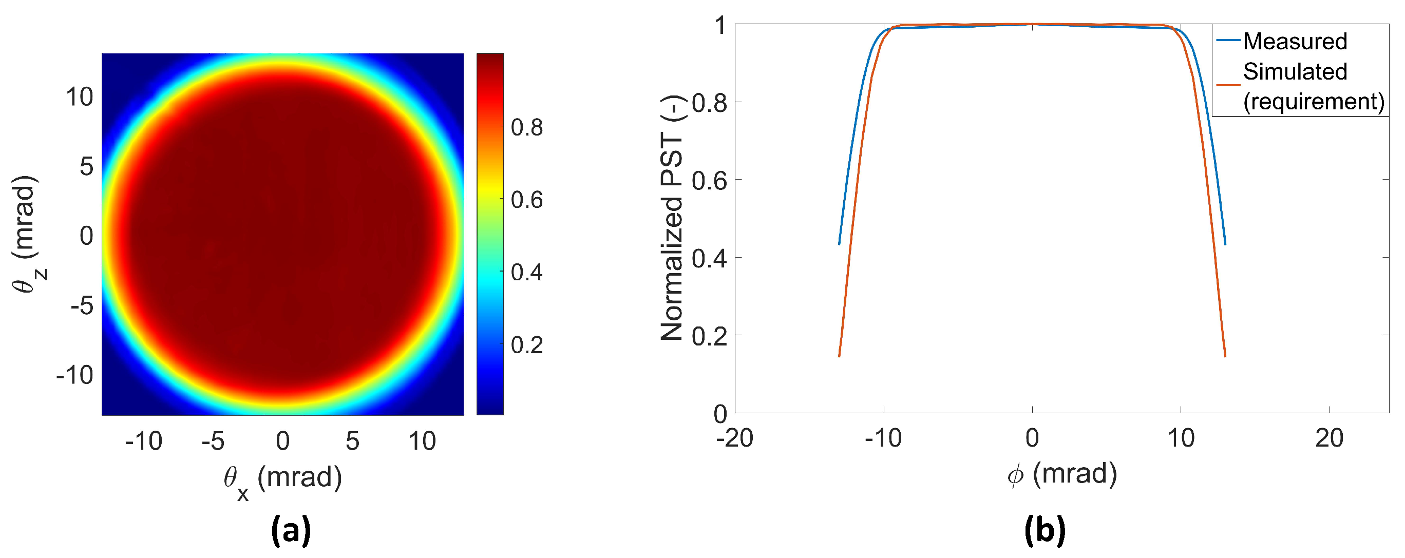
• The fiber has been aligned with the large GSE off-axis paraboloidal mirror with a precision that guarantees a beam divergence <0.35 mrad. Thus, the beam illuminating the receiver aperture during the receiver FOV characterization is not perfectly collimated, and the PST measurement within [–14, 14] mrad corresponds to the convolution of the beam divergence profile with the actual receiver FOV. Thus, there is a small artifact introduced in the measurements that leads to measuring a slightly larger FOV.
• Simulations assumed a perfect 2-mm diameter for the detector active area diameter, while in practice, there is an out-of-area (OOA) response: this is a contribution to the response from the area outside the 2-mm optical size if the detector is overfilled with illumination, due to the standard product design. In our case, the OOA is between 2.08 mm (inner diameter) and 2.125 mm (outer diameter) per detector mask design, with a responsivity within the OOA that can reach 90% of the responsivity in the central region of the active area.

6. Conclusions and Perspectives

Lunar Flashlight is a technology demonstration mission whose goal is to show that useful measurements can be made within very demanding CubeSat resource limitations at a much lower cost than previously possible. LF’s measurement goal is to measure the surface abundance of water ice on the lunar South Pole with concentrations of 5 wt% or less, down to as little as 0.5 wt%, with a spatial resolution of 10 km or better. Regions of interest are permanently shadowed and occasionally sunlit regions poleward of 80° S latitude. Previous missions have already demonstrated the likely presence of H₂O ice at the lunar poles, but have failed to accurately quantify its abundance and determine its form. Among the previous observations, the most relevant to LF are the surface reflectance variations measured by the LOLA 1064-nm laser altimeter [29] and the ice-like reflectance spectra measured by M3 [27]. These two observations verify that ice is likely present in sufficient quantities, such that Lunar Flashlight should be capable of detecting and quantifying ice abundance on the Moon’s surface.

This paper presents the optical, mechanical, and thermal designs of the Lunar Flashlight receiver subsystem, as well as its characterization. The receiver, as delivered, has been demonstrated to meet its flight requirements in terms of:

• field of view (requirement: 20 mrad with <3.7% non-uniformity within 100% of the FOV and <1.3% non-uniformity within 95% of the FOV; measurement: 20 mrad with 2% non-uniformity within 100% of the FOV, and 1.3% non-uniformity within 95% of the FOV);
• responsivity (requirements: >0.47 A/W at 1064 nm, >0.89 A/W at 1495 nm, >1.05 A/W at 1850 nm, >1.04 A/W at 1990 nm; measurements: 0.51 A/W at 1064 nm, 1.06 A/W at 1495 nm, 1.36 A/W at 1850 nm, and 1.37 A/W at 1990 nm);
• receiver dark current (requirement: <2 nA; measurement: 0.38 nA with the femtoammeter ground support equipment providing a bias <1 mV).

The NEP of the receiver detector (manufacturer specifications: 9.3×10^-14 W/$\sqrt{Hz}$ maximum, 6.6×10^-14 W/$\sqrt{Hz}$ typical at 2.06 μm, 208 K, and 1 kHz) has not been measured. The instrument noise is driven by the reading electronics of the receiver, which is currently in a redesign phase to maximize its SNR. The noise of the entire chain (receiver and its reading electronics) will be measured in the next few months.

The next steps will be to finalize the design of the analog electronics that is used to read the detector output current in order to maximize the instrument SNR, integrate and test the receiver with the rest of the instrument (lasers, flight electronics, batteries), measure the instrument SNR, evaluate the related water ice measurement performance (water ice discrimination level as a function of the confidence level and mapping resolution) to ensure that the instrument meets its requirements, and proceed to an end-to-end calibration of the entire instrument. The instrument will then be ready for integration and test (I&T) at the spacecraft level.

This highly mass-constrained and volume-constrained instrument payload will demonstrate several firsts, including being one of the first instruments onboard a CubeSat performing science measurements beyond low Earth orbit, and the first planetary mission to use multi-band active reflectometry from orbit.

References

1. Goddard, E.C. The Papers of Robert H. Goddard; Pendray, G.E., Ed.; McGraw-Hill: New York, NY, USA, 1970; Volume 1, pp. 1938–19845. [Google Scholar]
2. Watson, K.; Murray, B.; Brown, H. On the possible presence of ice on the Moon. J. Geophys. Res. 1961, 66, 1598–1600. [Google Scholar] [CrossRef] [Green Version]
3. Paige, D.A.; Siegler, M.A.; Zhang, J.A.; Hayne, P.O.; Foote, E.J.; Bennett, K.A.; Vasavada, A.R.; Greenhagen, B.T.; Schofield, J.T.; McCleese, D.J.; et al. Diviner lunar radiometer observations of cold traps in the Moon’s south polar region. Science 2010, 330, 479–482. [Google Scholar] [CrossRef] [PubMed]
4. Hayne, P.O.; Hendrix, A.; Sefton-Nash, E.; Siegler, M.A.; Lucey, P.G.; Retherford, K.D.; Williams, J.P.; Greenhagen, B.T.; Paige, D.A. Evidence for exposed water ice in the Moon’s south polar regions from Lunar Reconnaissance Orbiter ultraviolet albedo and temperature measurements. Icarus 2015, 255, 58–69. [Google Scholar] [CrossRef]
5. Hayne, P.O.; Paige, D.A.; Ingersoll, A.P.; Judd, M.A.; Aharonson, O.; Alkali, L.; Byrne, S.; Cohen, B.; Colaprete, A.; Combe, J.P.; et al. New Approaches to Lunar Ice Detection and Mapping: Study Overview and Results of the First Workshop. In Proceedings of the Annual Meeting of the Lunar Exploration Analysis Group, 14–16 October 2013; Volume 1748, p. 7043. [Google Scholar]
6. The Lunar Exploration Analysis Group (LEAG); The Mars Exploration Program Analysis Group (MEPAG); The Small Bodies Assessment Group (SBAG) Strategic Knowledge Gaps (SKGs). Available online: https://www.nasa.gov/exploration/library/skg.html (accessed on 2 October 2018).
7. Thomson, B.J.; Bussey, D.B.J.; Neish, C.D.; Cahill, J.T.S.; Heggy, E.; Kirk, R.L.; Patterson, G.W.; Raney, R.K.; Spudis, P.D.; Thompson, T.W.; et al. An upper limit for ice in Shackleton crater as revealed by LRO Mini-RF orbital radar. Geophys. Res. Lett. 2012, 39. [Google Scholar] [CrossRef] [Green Version]
8. Spudis, P.D.; Bussey, D.B.J.; Baloga, S.M.; Cahill, J.T.S.; Glaze, L.S.; Patterson, G.W.; Raney, R.K.; Thompson, T.W.; Thomson, B.J.; Ustinov, E.A. Evidence for water ice on the Moon: Results for anomalous polar craters from the LRO Mini-RF imaging radar. J. Geophys. Res. Planets 2013, 118, 2016–2029. [Google Scholar] [CrossRef] [Green Version]
9. Nozette, S.; Lichtenberg, C.L.; Spudis, P.; Bonner, R.; Ort, W.; Malaret, E.; Robinson, M.; Shoemaker, E.M. The Clementine bistatic radar experiment. Science 2016, 274, 1495–1498. [Google Scholar] [CrossRef]
10. Feldman, W.C.; Maurice, S.; Binder, A.B.; Barraclough, B.L.; Elphic, R.C.; Lawrence, D.J. Fluxes of fast and epithermal neutrons from Lunar Prospector: Evidence for water ice at the lunar poles. Science 1998, 281, 1496–1500. [Google Scholar] [CrossRef] [PubMed]
11. Feldman, W.C.; Lawrence, D.J.; Elphic, R.C.; Barraclough, B.L.; Maurice, S.; Genetay, I.; Binder, A.B. Polar hydrogen deposits on the Moon. J. Geophys. Res. 2000, 105, 4175–4195. [Google Scholar] [CrossRef] [Green Version]
12. Feldman, W.C.; Lawrence, D.J.; Little, R.C.; Lawson, S.L.; Gasnault, O.; Wiens, R.C.; Barraclough, B.L.; Elphic, R.C.; Prettyman, T.H.; Steinberg, J.T. Evidence for water ice near the lunar poles. J. Geophys. Res. 2001, 106, 23231–23251. [Google Scholar] [CrossRef] [Green Version]
13. Mitrofanov, I.G.; Sanin, A.B.; Boynton, W.V.; Chin, G.; Garvin, J.B.; Golovin, D.; Evans, L.G.; Harshman, K.; Kozyrev, A.S.; Litvak, M.L.; et al. Hydrogen mapping of the lunar south pole using the LRO neutron detector experiment LEND. Science 2010, 330, 483–486. [Google Scholar] [CrossRef] [PubMed]
14. Mitrofanov, I.; Litvak, M.; Sanin, A.; Malakhov, A.; Golovin, D.; Boynton, W.; Droege, G.; Chin, G.; Evans, L.; Harshman, K.; et al. Testing polar spots of water-rich permafrost on the Moon: LEND observations onboard LRO. J. Geophys. Res. Planets 2012, 117. [Google Scholar] [CrossRef] [Green Version]
15. Boynton, W.V.; Droege, G.F.; Mitrofanov, I.G.; McClanahan, T.P.; Sanin, A.B.; Litvak, M.L.; Schaffner, M.; Chin, G.; Evans, L.G.; Garvin, J.B.; et al. High spatial resolution studies of epithermal neutron emission from the lunar poles: Constraints on hydrogen mobility. J. Geophys. Res. Planets 2012, 117. [Google Scholar] [CrossRef]
16. Livengood, T.A.; Chin, G.; Sagdeev, R.Z.; Mitrofanov, I.G.; Boynton, W.V.; Evans, L.G.; Litvak, M.L.; McClanahan, T.P.; Sanin, A.B.; Starr, R.D. Evidence for Diurnally Varying Hydration at the Moon’s Equator from the Lunar Exploration Neutron Detector (LEND). In Proceedings of the 45th Lunar and Planetary Science Conference, The Woodlands, TX, USA, 17–21 March 2014; p. 1507. [Google Scholar]
17. Schwadron, N.A.; Wilson, J.K.; Looper, M.D.; Jordan, A.P.; Spence, H.E.; Blake, J.B.; Case, A.W.; Iwata, Y.; Kasper, J.C.; Farrell, W.M.; et al. Signatures of volatiles in the lunar proton albedo. Icarus 2016, 273, 25–35. [Google Scholar] [CrossRef]
18. Gladstone, G.R.; Retherford, K.D.; Egan, A.F.; Kaufmann, D.E.; Miles, P.F.; Parker, J.W.; Horvath, D.; Rojas, P.M.; Versteeg, M.H.; Davis, M.W.; et al. Far-ultraviolet reflectance properties of the Moon’s permanently shadowed regions. J. Geophys. Res. Planets 2012, 117. [Google Scholar] [CrossRef]
19. Hendrix, A.R.; Retherford, K.D.; Randall Gladstone, G.; Hurley, D.M.; Feldman, P.D.; Egan, A.F.; Kaufmann, D.E.; Miles, P.F.; Parker, J.W.; Horvath, D.; et al. The lunar far-UV albedo: Indicator of hydration and weathering. J. Geophys. Res. Planets 2012, 117. [Google Scholar] [CrossRef] [Green Version]
20. Colaprete, A.; Schultz, P.; Heldmann, J.; Wooden, D.; Shirley, M.; Ennico, K.; Hermalyn, B.; Marshall, W.; Ricco, A.; Elphic, R.C.; et al. Detection of water in the LCROSS ejecta plume. Science 2012, 330, 463–468. [Google Scholar] [CrossRef] [PubMed]
21. Heldmann, J.L.; Lamb, J.; Asturias, D.; Colaprete, A.; Goldstein, D.B.; Trafton, L.M.; Varghese, P.L. Evolution of the dust and water ice plume components as observed by the LCROSS visible camera and UV-visible spectrometer. Icarus 2015, 254, 262–275. [Google Scholar] [CrossRef]
22. Pieters, C.M.; Goswami, J.N.; Clark, R.N.; Annadurai, M.; Boardman, J.; Buratti, B.; Combe, J.P.; Dyar, M.D.; Green, R.; Head, J.W.; et al. Character and spatial distribution of OH/H2O on the surface of the Moon seen by M3 on Chandrayaan-1. Science 2009, 326, 568–572. [Google Scholar] [CrossRef]
23. Sunshine, J.M.; Farnham, T.L.; Feaga, L.M.; Groussin, O.; Merlin, F.; Milliken, R.E.; A’Hearn, M.F. Temporal and spatial variability of lunar hydration as observed by the Deep Impact spacecraft. Science 2009, 326, 565–568. [Google Scholar] [CrossRef]
24. Clark, R.N. Detection of adsorbed water and hydroxyl on the Moon. Science 2009, 326, 562–564. [Google Scholar] [CrossRef]
25. Zuber, M.T.; Head, J.W.; Smith, D.E.; Neumann, G.A.; Mazarico, E.; Torrence, M.H.; Aharonson, O.; Tye, A.R.; Fassett, C.I.; Rosenburg, M.A.; et al. Constraints on the volatile distribution within Shackleton crater at the lunar south pole. Nature 2012, 486, 378–381. [Google Scholar] [CrossRef] [Green Version]
26. Lucey, P.G.; Neumann, G.A.; Paige, D.A.; Riner, M.A.; Mazarico, E.M.; Smith, D.E.; Zuber, M.T.; Siegler, M.; Hayne, P.O.; Bussey, D.B.J.; et al. Evidence for Water Ice and Temperature Dependent Space Weathering at the Lunar Poles from Lola and diviners. In Proceedings of the 45th Lunar and Planetary Science Conference, The Woodlands, TX, USA, 17–21 March 2014; p. 2325. [Google Scholar]
27. Li, S.; Lucey, P.G.; Milliken, R.E.; Hayne, P.O.; Fisher, E.; Williams, J.P.; Hurley, D.M.; Elphic, R.C. Direct evidence of surface exposed water ice in the lunar polar regions. Proc. Natl. Acad. Sci. USA 2018, 115. [Google Scholar] [CrossRef]
28. Hayne, P.O.; Cohen, B.A.; Sellar, R.G.; Staehle, R.; Toomarian, N.; Paige, D.A. Lunar flashlight: Mapping lunar surface volatiles using a cubesat. In Proceedings of the Annual Meeting of the Lunar Exploration Analysis Group, Laurel, MD, USA, 14–16 October 2013; p. 7045. [Google Scholar]
29. Fisher, E.A.; Lucey, P.G.; Lemelin, M.; Greenhagen, B.T.; Siegler, M.A.; Mazarico, E.; Aharonson, O.; Williams, J.P.; Hayne, P.O.; Neumann, G.A.; et al. Evidence for surface water ice in the lunar polar regions using reflectance measurements from the Lunar Orbiter Laser Altimeter and temperature measurements from the Diviner Lunar Radiometer Experiment. Icarus 2017, 292, 74–85. [Google Scholar] [CrossRef]
30. Smith, D.E.; Zuber, M.T.; Neumann, G.A.; Lemoine, F.G.; Mazarico, E.; Torrence, M.H.; McGarry, J.F.; Rowlands, D.D.; Head, J.W.; Duxbury, T.H.; et al. Initial observations from the lunar orbiter laser altimeter (LOLA). Geophys. Res. Lett. 2010, 37. [Google Scholar] [CrossRef]
31. Riris, H.; Cavanaugh, J.; Sun, X.; Liiva, P.; Rodriguez, M.; Neuman, G. The lunar orbiter laser altimeter (LOLA) on NASA’s lunar reconnaissance orbiter (LRO) mission. In Proceedings of the International Conference on Space Optics, Rhodes Island, Greece, 4–8 October 2010. [Google Scholar]
32. Ramos-Izquierdo, L.; Scott, V.S., III; Connelly, J.; Schmidt, S.; Mamakos, W.; Guzek, J.; Peters, C.; Liiva, P.; Rodriguez, M.; Cavanaugh, J.; et al. Optical system design and integration of the Lunar Orbiter Laser Altimeter. Appl. Opt. 2009, 48, 3035–3049. [Google Scholar] [CrossRef] [PubMed]
33. Cohen, B.A.; Hayne, P.O.; Greenhagen, B.T.; Paige, D.A.; Camacho, J.M.; Crabtree, K.; Paine, C.G.; Sellar, R.G. Payload Design for the Lunar Flashlight Mission. In Proceedings of the 48th Lunar and Planetary Science Conference, The Woodlands, TX, USA, 20–24 March 2017; p. 1709. [Google Scholar]
34. Wehmeier, U.; Vinckier, Q.; Sellar, R.G.; Paine, C.G.; Hayne, P.O.; Bagheri, M.; Rais-Zadeh, M.; Forouhar, S.; Loveland, J.; Shelton, J. The Lunar Flashlight CubeSat instrument: A compact SWIR laser reflectometer to quantify and map water ice on the surface of the Moon. In Proceedings of the SPIE Optical Engineering + Application conference—CubeSats and NanoSats for Remote Sensing II, San Diego, CA, USA, 21–22 August 2018; Volume 10769, p. 107690H. [Google Scholar]
35. Lucey, P.G.; Sun, X.; Abshire, J.B.; Neumann, G.A. An orbital lidar spectrometer for lunar polar compositions. In Proceedings of the 45th Lunar and Planetary Science Conference, The Woodlands, TX, USA, 17–21 March 2014; p. 2335. [Google Scholar]
36. Robinson, K.F.; Norris, G. NASA’s Space Launch System: Deep-Space Delivery for Smallsats. In Proceedings of the Annual AIAA Space and Astronautics Forum and Exposition, Orlando, FL, USA, 12–14 September 2017; p. M17-6183. [Google Scholar]
37. Clark, P.E.; Malphrus, B.; Brown, K.; Hurford, T.; Brambora, C.; MacDowall, R.; Folta, D.; Tsay, M.; Brandon, C.; Team, L.I.C. Lunar Ice Cube: Searching for Lunar Volatiles with a lunar cubesat orbiter. In Proceedings of the 48th Meeting of the Division for Planetary Sciences, Pasadena, CA, USA, 16–21 October 2016. [Google Scholar]
38. Hardgrove, C.; Bell, J.; Thangavelautham, J.; Klesh, A.; Starr, R.; Colaprete, T.; Robinson, M.; Drake, D.; Johnson, E.; Christian, J.; et al. The Lunar Polar Hydrogen Mapper (LunaH-Map) mission: Mapping hydrogen distributions in permanently shadowed regions of the Moon’s south pole. In Proceedings of the Annual Meeting of the Lunar Exploration Analysis Group, Columbia, MD, USA, 20–22 October 2015; Volume 1863, p. 2035. [Google Scholar]
39. Lunar Flashlight Propulsion System. Available online: https://www.cubesat-propulsion.com/wp-content/uploads/2017/08/X16029000-01-data-sheet-080217.pdf (accessed on 3 October 2018).
40. Kobayashi, M. Iris Deep-Space Transponder for SLS EM-1 CubeSat Missions. In Proceedings of the AIAA/USU Conference on Small Satellites, Logan, UT, USA, 5–10 August 2017; p. SSC17-II-04. [Google Scholar]
41. Vinckier, Q.; Crabtree, K.; Gibson, M.; Smith, C.; Wehmeier, U.; Hayne, P.O.; Sellar, R.G. Optical and mechanical designs of the multi-band SWIR receiver for the Lunar Flashlight CubeSat mission. In Proceedings of the SPIE Optical Systems Design conference—Optical Design and Engineering VII, Frankfurt, Germany, 5 June 2018; Volume 10690, p. 106901I. [Google Scholar]
42. Vinckier, Q.; Hayne, P.O.; Martinez-Camacho, J.M.; Paine, C.; Cohen, B.A.; Wehmeier, U.J.; Sellar, R.G. System Performance Modeling of the Lunar Flashlight CubeSat Instrument. In Proceedings of the 49th Lunar and Planetary Science Conference, The Woodlands, TX, USA, 19–23 March 2018; p. 1030. [Google Scholar]
43. Hapke, B. Bidirectional reflectance spectroscopy: 1. Theory. J. Geophys. Res. Solid Earth 1981, 86, 3039–3054. [Google Scholar] [CrossRef]
44. Warren, S.G.; Richard, E.B. Optical constants of ice from the ultraviolet to the microwave: A revised compilation. J. Geophys. Res. Atmos. 2008, 113. [Google Scholar] [CrossRef] [Green Version]
45. NASA Jet Propulsion Laboratory—California Institute of Technology: Lunar Flashlight CubeSat Mission. Available online: https://www.jpl.nasa.gov/cubesat/missions/lunar_flashlight.php (accessed on 5 November 2018).
46. Harvey, J. Light Scattering Characteristics of Optical Surfaces. Ph.D. Thesis, University of Arizona, Tucson, AZ, USA, 1976. [Google Scholar]
47. Military Standard 1246C. Product Cleanliness Levels and Contamination Control Program. In Technical Report; Department of Defense: Washington, DC, USA, 1994. [Google Scholar]
48. Harvey, J.E.; Choi, N.; Schroeder, S.; Duparré, A. Total integrated scatter from surfaces with arbitrary roughness, correlation widths, and incident angles. Opt. Eng. 2012, 51, 013402. [Google Scholar] [CrossRef]
Figure 1. Lunar Flashlight (LF) CubeSat. (a) LF CubeSat with solar panels deployed [34]; (b) LF CubeSat stowed [34]; (c) LF instrument: shortwave infrared (SWIR) laser reflectometer [41].
Remotesensing 11 00440 g001
Figure 2. Block diagram of the Lunar Flashlight payload.
Remotesensing 11 00440 g002
Figure 3. Reflectance spectrum (bidirectional reflectance) for different weight percentages of water ice (wt%) in lunar regolith at zero-phase angle [41,42]. We calculated these model spectra using Hapke theory [43], with water ice optical constants from Warren et al. [44], and a reflectance spectrum of the Apollo 14 lunar highlands sample 14259-85.
Remotesensing 11 00440 g003
Figure 4. Mission design. (a) Proposed LF lunar orbit (not to scale; DSN: deep space network) [34]; (b) LF spacecraft science data paths on the lunar South Pole [34,42]. The gray scale shows the maximum temperature; the green and pink segments are the science paths, with the pink dots indicating the Permanently Shadowed Regions (PSRs). The total duration of the science data paths is equal to approximately 39 minutes, with approximately 5 minutes corresponding to measurements over PSRs.
Remotesensing 11 00440 g004
Figure 5. Instrument operation concept (not to scale; figure updated from [41]). The four different wavelengths emitted by the lasers are illustrated by the four different colors of the pulses.
Remotesensing 11 00440 g005
Figure 6. Measured far-field normalized laser divergence profiles. The color scales report the lasers’ radiances normalized to unity. θx and θz are respectively the rotation angles around axis X and Z, and the XZ plane is coplanar with the optical window of the laser package. The lasers’ co-alignment is thus “included” in the data depicted in this figure. These data come from DILAS Inc., which has designed the lasers. The coordinate (0,0) mrad corresponds to the centroid of the average of the divergence beam profiles depicted in Figure 10(b). The difference between the laser divergence profiles leads to small differences in the footprint on the lunar surface for each wavelength, but this has minimal importance, since LF’s goal is to measure the average water ice concentration over distances up to 10 km long.
Remotesensing 11 00440 g006
Figure 7. Solar stray light reflected toward the receiver aperture and scattered onto the detector active area from outside the field of view (FOV) during a PSR observation on the Moon (not to scale; artistic view inspired by [45]). The blue cone represents the receiver FOV (not to scale).
Remotesensing 11 00440 g007
Figure 8. Receiver vanes’ configuration [41].
Remotesensing 11 00440 g008
Figure 9. Rotational average of the simulated receiver point source transmittance (PST) function. The maximum value of the simulated PST function is equal to 0.679 (67.9% of the light passing through the receiver aperture reaches the detector active area). The corresponding 32.1% of optical losses are due to the following. (1) The PST calculation is normalized to the flux passing through an unobscured 75-mm square entrance aperture, rather than the smaller and more complex mirror shape of the actual receiver. (2) The Al mirror reflectivity is modeled as 94.5% at a wavelength of 1 µm. (3) The detector surface reflectivity is modeled as 3%. (4) The losses due to vignetting by the detector housing (which obstructs a part of the receiver aperture) [41]. The modeled reflectivity of bare Al at 1 µm comes from the database used by the ray-tracing software FRED. Reflectivity at 1.495 µm is equal to 97.7%, and reflectivity at 1.850 µm and 1.990 µm is equal to 98%.
Remotesensing 11 00440 g009
Figure 10. (a) Receiver PST function within [–15, 15] mrad angular range [41]; (b) Measured normalized averaged divergence beam profiles of the lasers [34]. The black circle on both figures corresponds to the uniform 20-mrad receiver FOV.
Remotesensing 11 00440 g010
Figure 11. LF reflectometer assembly (three-dimensional model) (figure updated from [41]). The reflectometer assembly is attached semi-kinematically through the rigid phase-change material (PCM) chassis mounting features to the X and Y structural panels of the spacecraft.
Remotesensing 11 00440 g011
Figure 12. Receiver module with cryoradiator (left) and section view (right) showing fastener detail of semi-kinematic snap-together design (figure updated from [41]).
Remotesensing 11 00440 g012
Figure 13. Detector semi-kinematic attachment to the receiver housing (top left), detector assembly section view (lower left), receiver section view (top right), and detailed three-dimensional (3D) view of the detector assembly (lower right) (figure updated from [41]).
Remotesensing 11 00440 g013
Figure 14. Connection of the receiver module to the PCM chassis via the six stinger flexures with pairs oriented for tip–tilt adjustment relative to laser module boresight.
Remotesensing 11 00440 g014
Figure 15. LF reflectometer optomechanical assembly (flight hardware). The receiver aperture and the laser package optical window are covered with a temporary clean static shielding sheet to protect the receiver mirror and the laser module’s optical window from particulates.
Remotesensing 11 00440 g015
Figure 16. Measured receiver and cryoradiator dimensions in mm. The dimensions given in parenthesis correspond to the ones on the drawings that exclude the electroplated gold layer.
Remotesensing 11 00440 g016
Figure 17. Receiver spectral calibration bench. The temperature of the detector and the receiver housing and mirror were stabilized independently using a cryogenic cooling system, several electric heaters, and two temperature sensors interfaced to a proportional–integral–derivative (PID) regulator (Lake Shore 340). Before the light enters the monochromator entrance slit, it passes through a long-pass filter. A 950-nm cut-on wavelength long-pass filter was used when working with the 1064-nm and 1495-nm wavelengths, and a 1450-nm cut-on wavelength long-pass filter was used when working with the 1850-nm and 1990-nm wavelengths. These long-pass filters were used to eliminate the lower wavelength light that the monochromator couples into from the second-order reflection of the grating.
Remotesensing 11 00440 g017
Figure 18. LF reflectometer optomechanical assembly in the vacuum chamber. 1: thermal strap mounted on the cryoradiator to control the temperature of the science detector; 2: thermal strap mounted on the receiver housing to control the temperature of the receiver mirror; 3: electrical heaters; 4: cold points inside the vacuum chamber; 5: optical window; 6: kinematic mount of the reflective collimator; 7: vacuum chamber feedthrough to connect the science detector to the femtoammeter.
Remotesensing 11 00440 g018
Figure 19. Receiver FOV characterization bench. Monochromator: “SDMC1-06G #95 850-2.2u” monochromator from Optometrics aligned with a “TS-20W” tungsten lamp and controlled by a “PCM-02 110V” stepping motor controller (stepper motor was positioned to output the zero-order diffraction); Fiber at the output of the monochromator: “FG200LEA” multimode fiber from Thorlabs, 0.22 numerical aperture, Low-OH, Ø200-µm Core, 400–2400 nm; Fiber at the focal position of the ground support equipment (GSE) off-axis paraboloidal mirror: 60-µm square core fiber provided by Molex, 102-µm cladding, 0.195 numerical aperture; GSE off-axis paraboloidal mirror: 101.6-mm diameter, 516.8-mm effective focal length, 15°, 100 Å roughness, protected aluminum off-axis paraboloidal mirror from Edmund Optics; two-axis gimbal: based on two X-RSW60A motorized rotation stages provided by Zaber technologies Inc.; Femtoammeter: “Keithley 6430” with its remote pre-amplifier.
Remotesensing 11 00440 g019
Figure 20. Receiver FOV characterization. (a) Normalized two-dimensional (2D) PST within [–14, 14] mrad angular range; (b) rotationally average of the normalized 2D PST within [–14, 14] mrad angular range and comparison with simulation. Measured receiver FOV: 20 mrad with 2% non-uniformity within 100% of the FOV and 1.3% non-uniformity within 95% of the FOV.
Remotesensing 11 00440 g020