Galileo Augmenting GPS Single-Frequency Single-Epoch Precise Positioning with Baseline Constrain for Bridge Dynamic Monitoring

 , , ,
, , ,
Abstract
:1. Introduction
2. SFSE Double-Differenced GPS/Galileo Mathematical Model
2.1. Single GPS/Galileo Code and Phase Observation Equations
2.2. Integrated GPS/Galileo Code and Phase Observation Equations
2.2.1. GPS/Galileo Loosely Combined Mode (LCM)
2.2.2. GPS/Galileo Tightly Combined Mode (TCM) with Differential Inter-system Biases (DISBs)
2.2.3. GPS/Galileo Tightly Combined Mode (TCM) without Inter-System Biases (ISBs)
2.3. Stochastic Model
2.4. Baseline Length Constraint DD Positioning Method
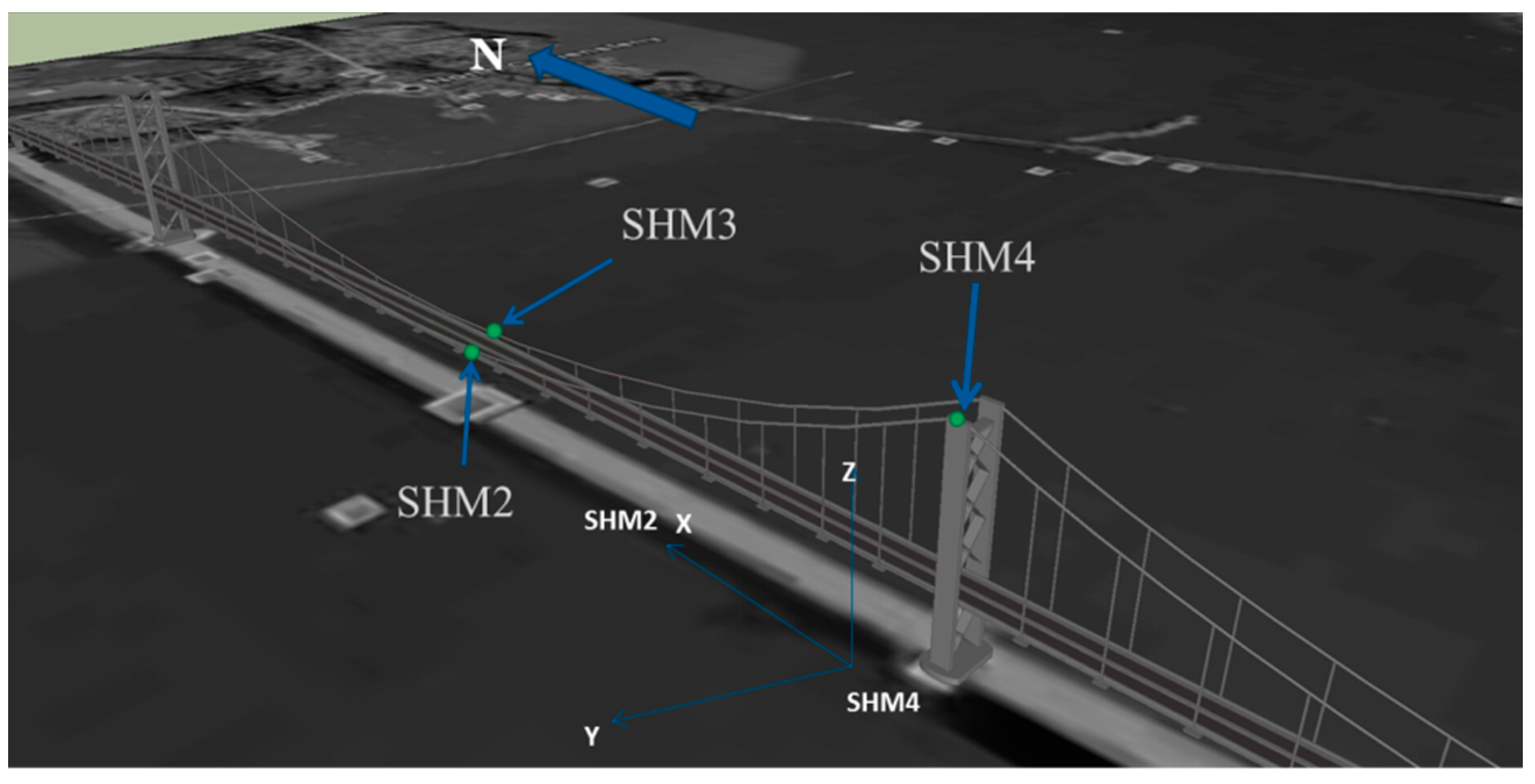
3. Monitoring Data Collecting for the Forth Bridge
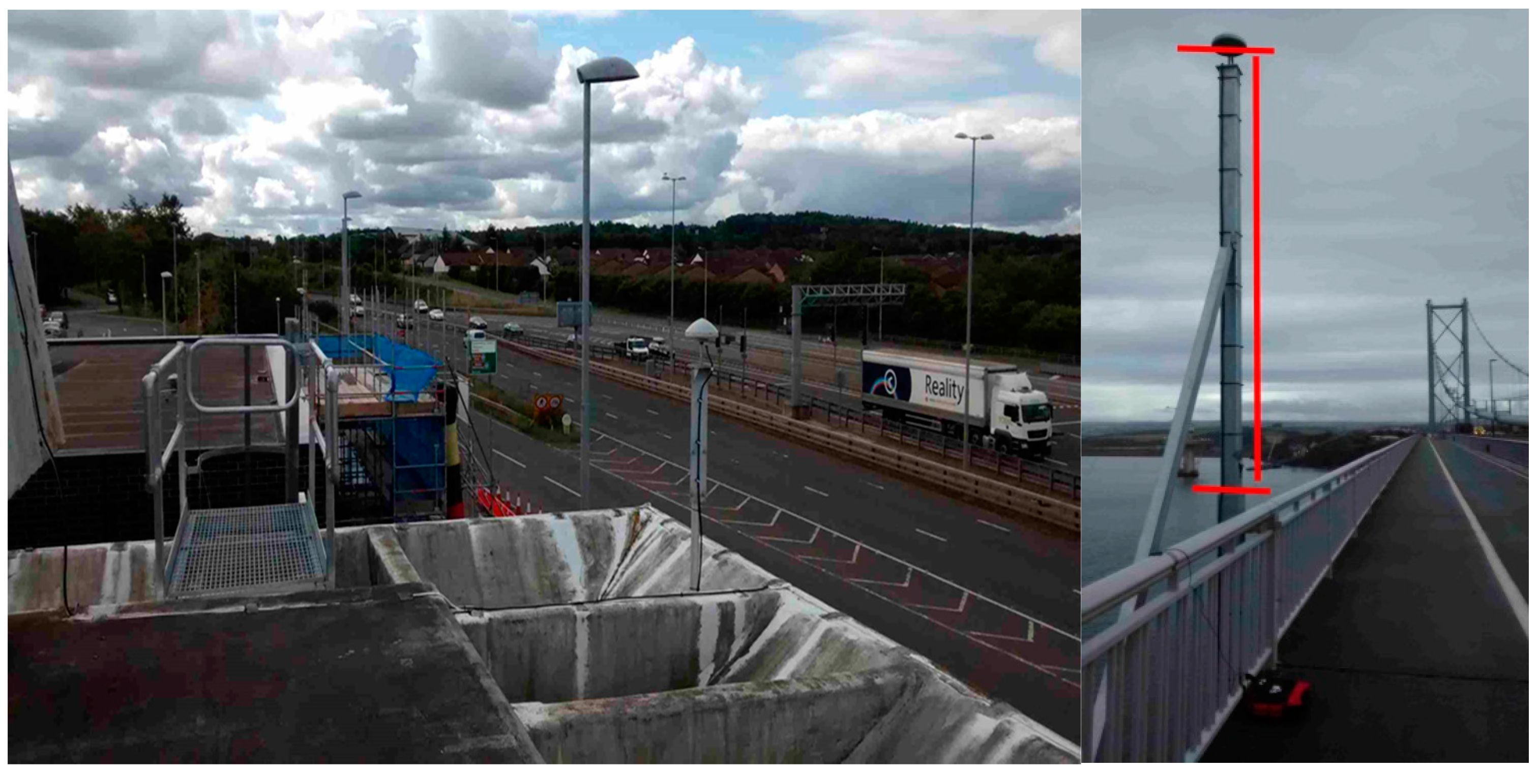
3.1. Data Collecting
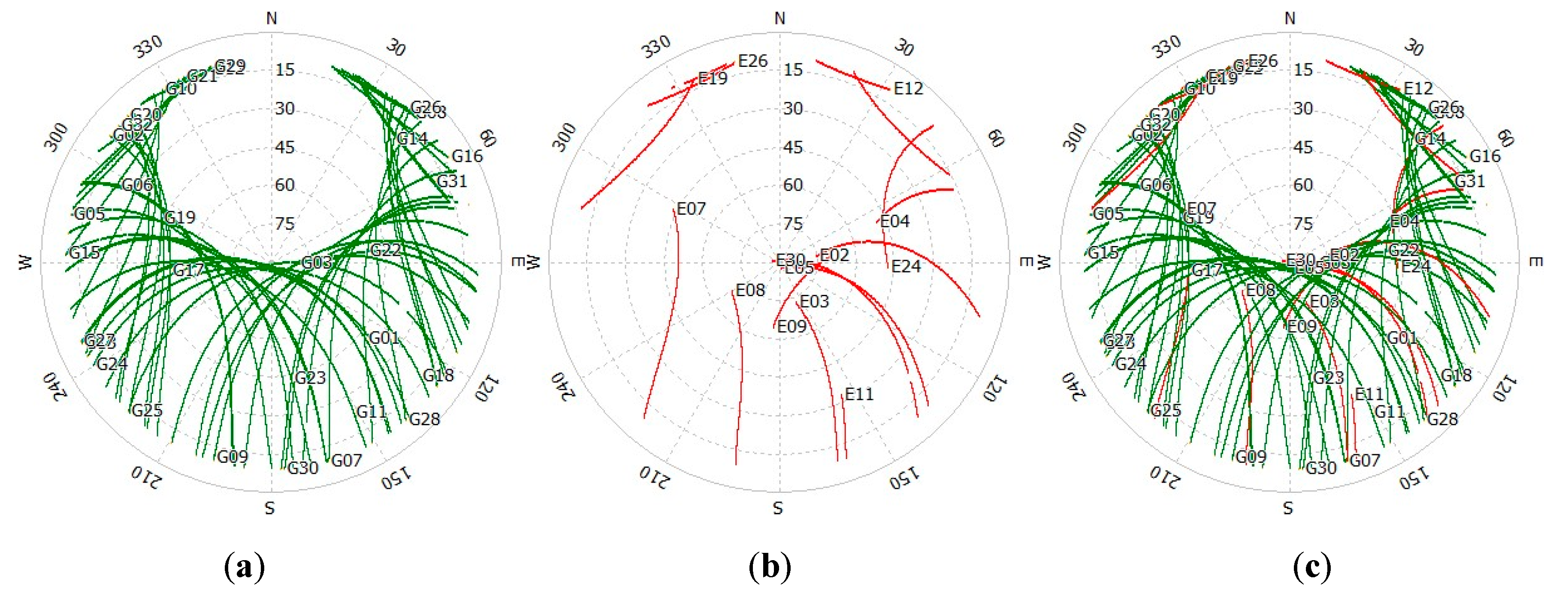
3.2. Sky Plots
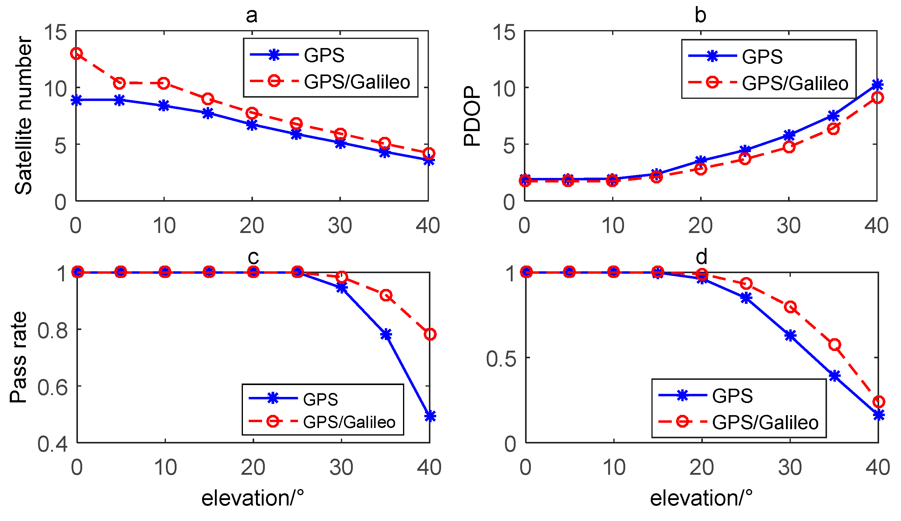
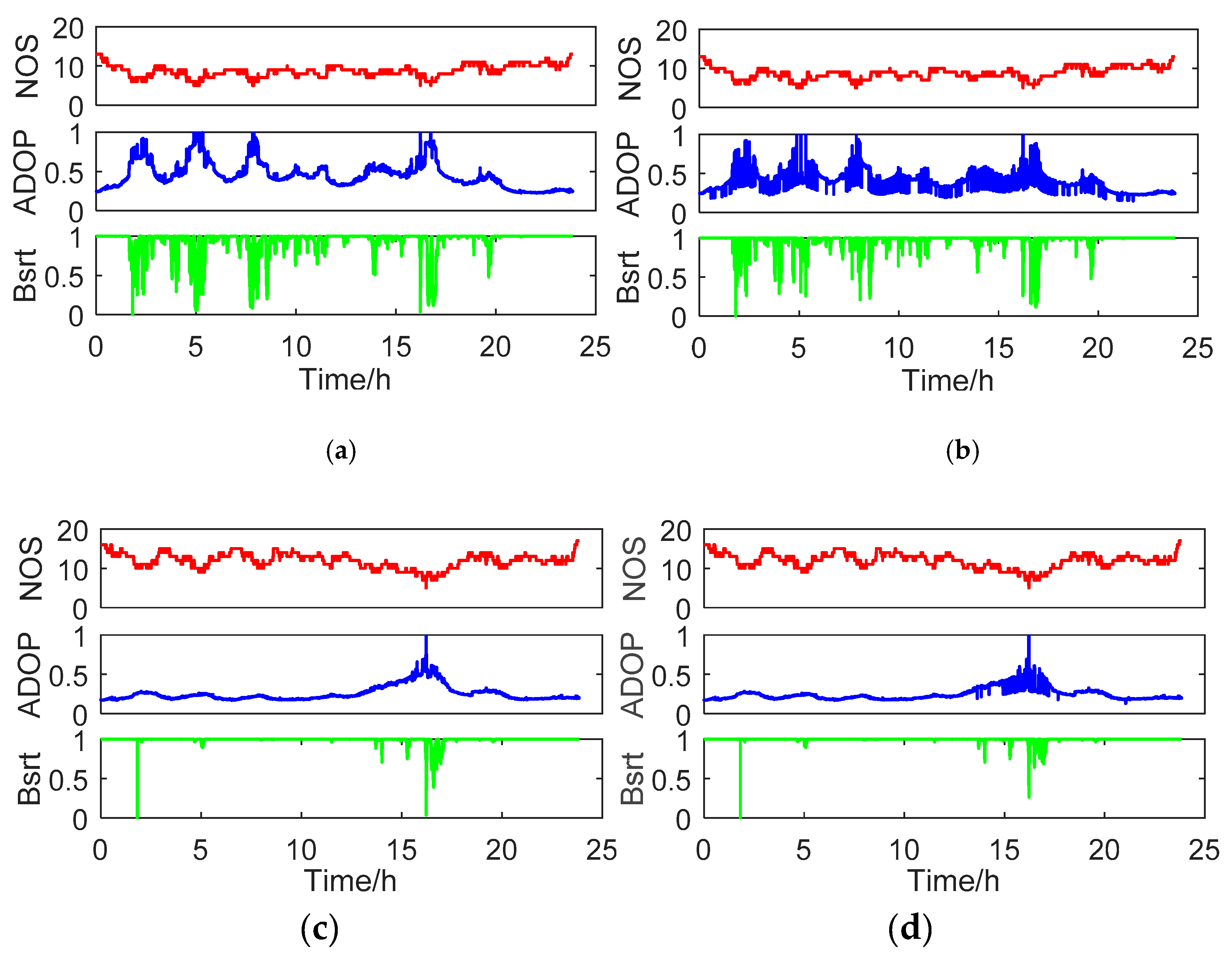
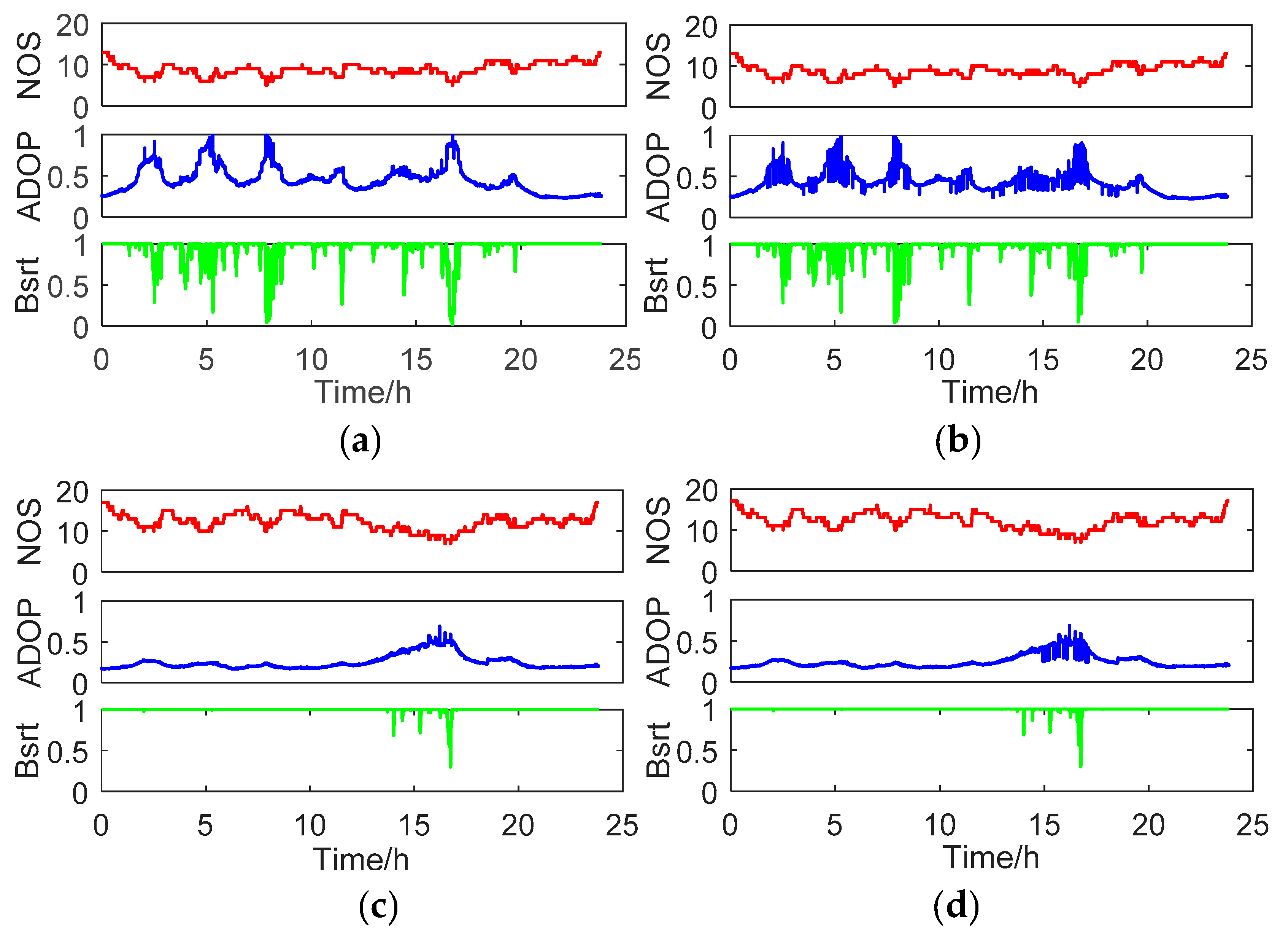
3.3. Availability and PDOP
4. Galileo Augmenting GPS SFSE Precise Positioning Experiment
4.1. Evaluation Index
4.2. Experiment Analysis
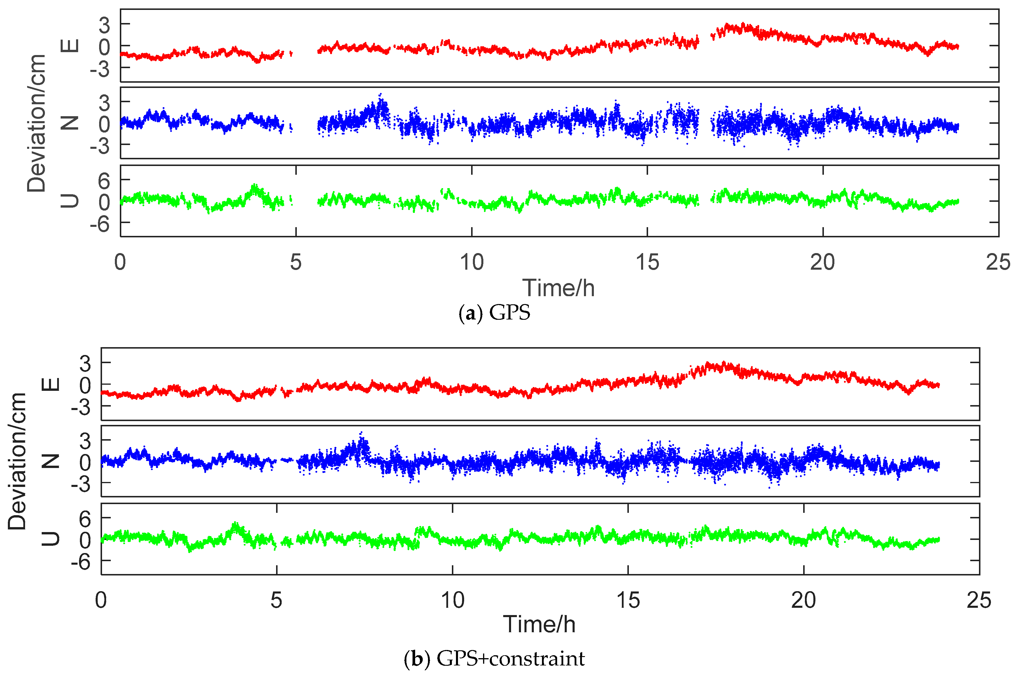
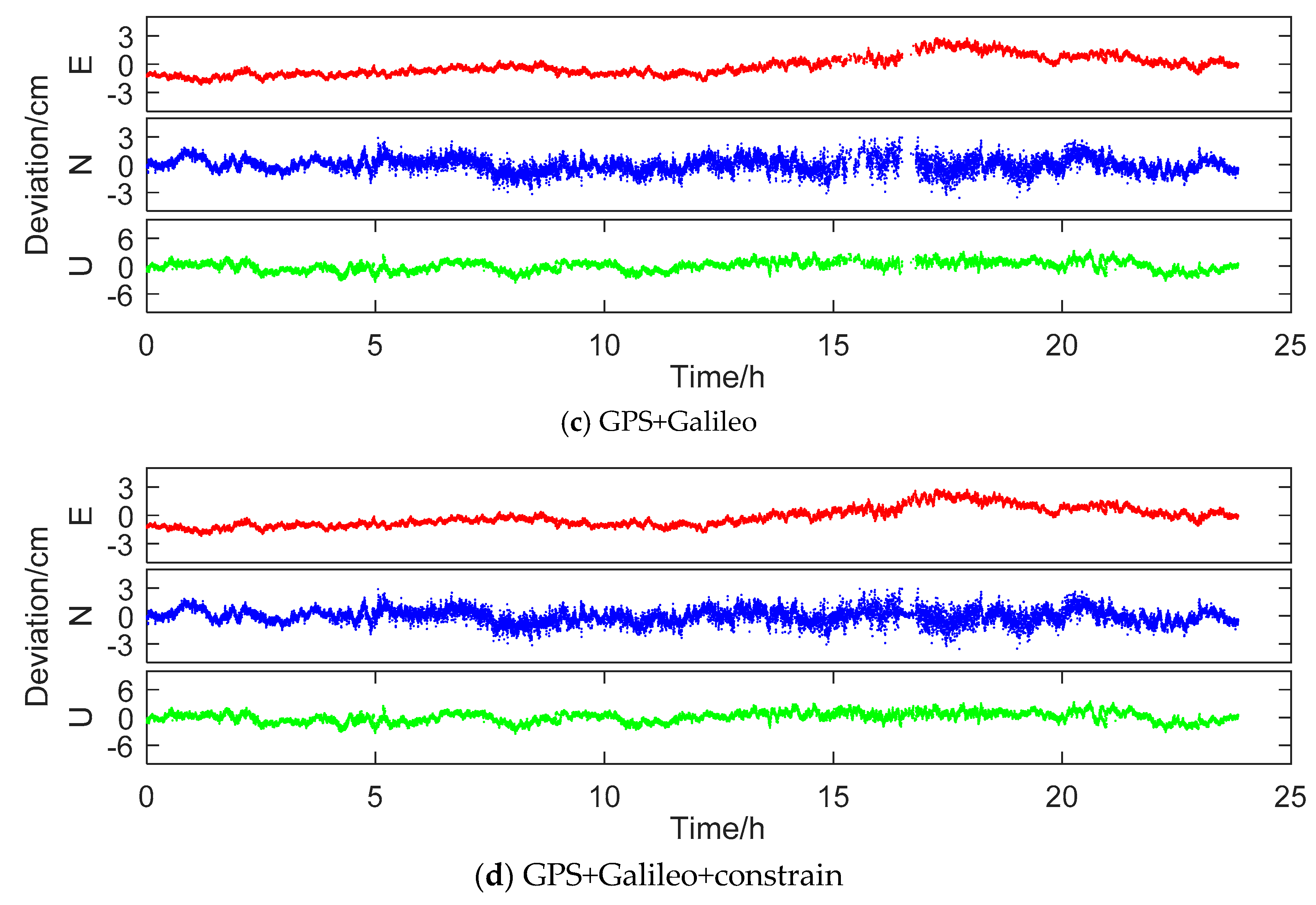
4.2.1. Experiment 1
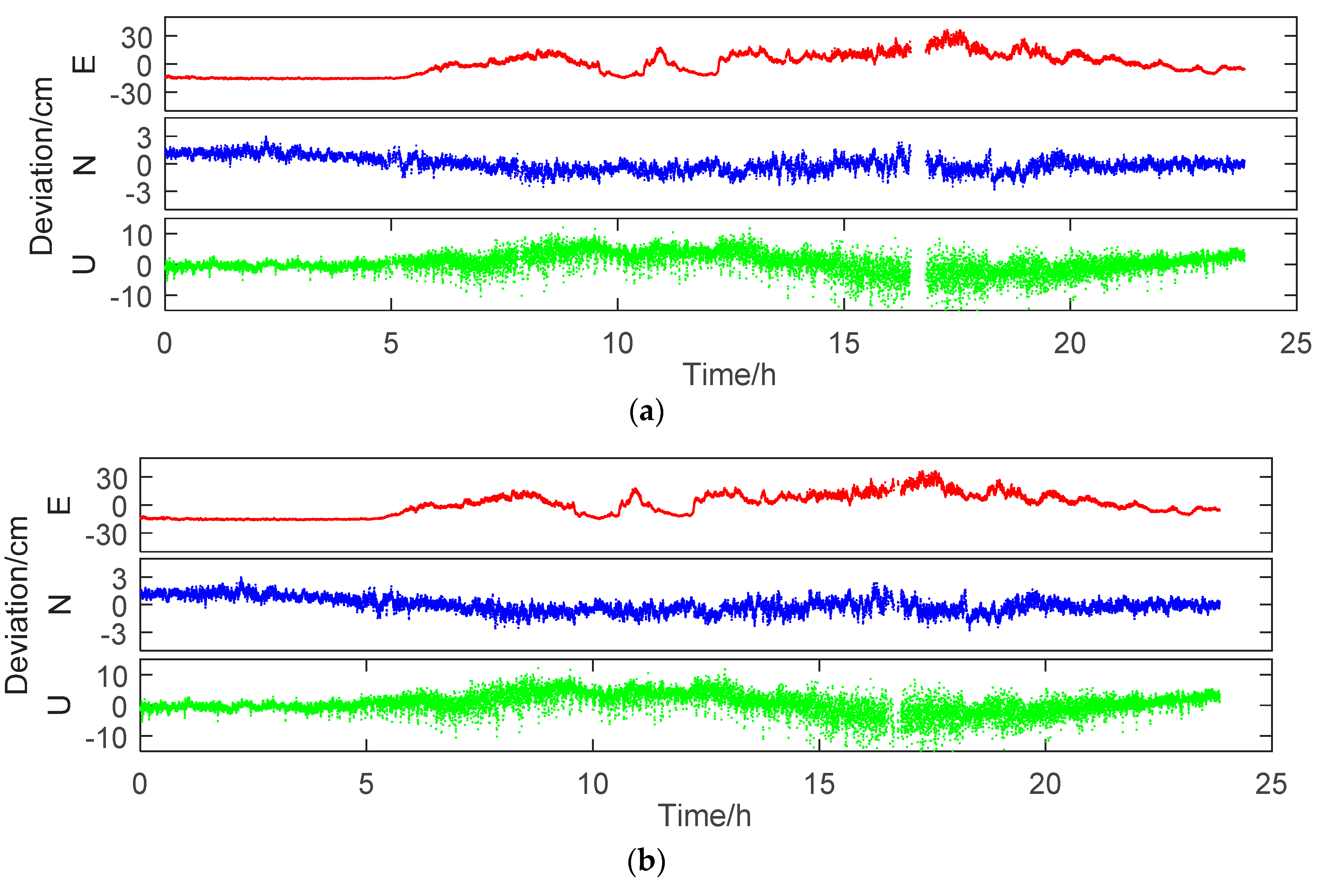
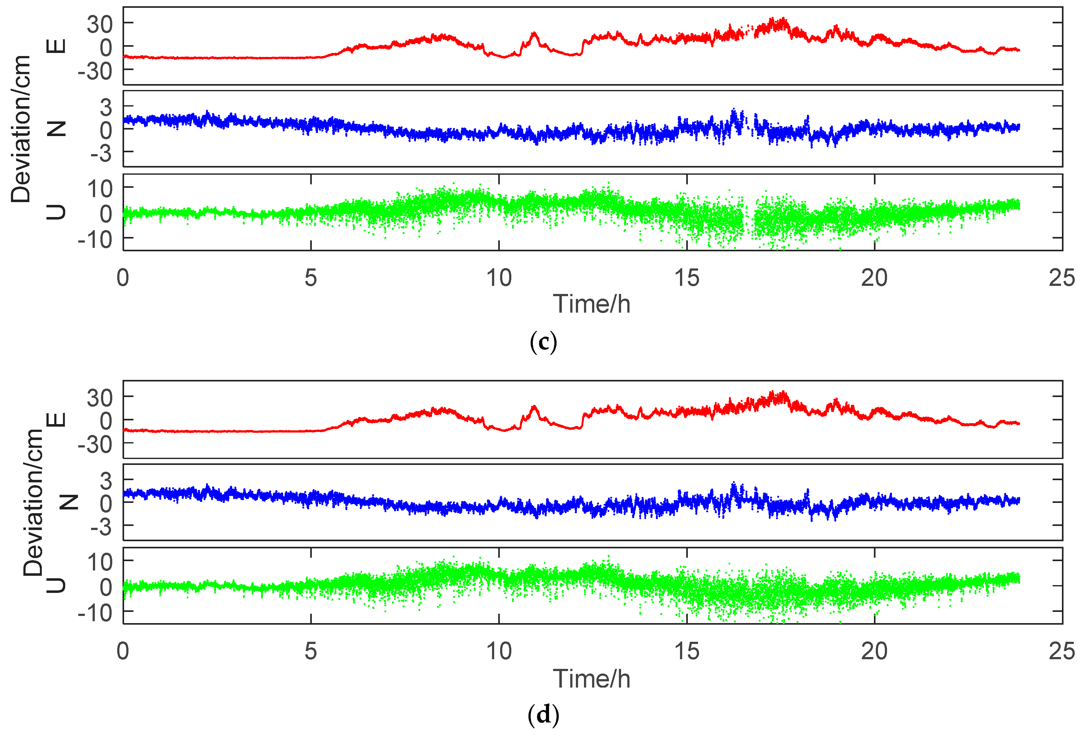
4.2.2. Experiment 2
5. Conclusions
Author Contributions
Funding
Acknowledgments
Conflicts of Interest
Abbreviations
| Abbreviation | Full name |
| ADOP | ambiguity dilution of precision |
| Asrt | actual success rate |
| BCS | Bridge Coordinate System |
| BDS | BeiDou Satellite Navigation System |
| Bsrt | bootstrapped success rate |
| BSSD | between-satellite single-difference |
| C/N0 | carrier-to-noise density ratio |
| C-GPS | GPS with baseline constraint |
| C-GPS/Galileo | GPS/Galileo with baseline constraint |
| DD | double-differenced |
| DISBs | inter-system biases |
| FFT | Fast Fourier Transformation |
| Galileo | Galileo Satellite Navigation System |
| GeoSHM | The GNSS and Earth Observation for Structural Health Monitoring |
| GGTO | GPS-to-Galileo Time Offset |
| GNSS | Global Navigation Satellite System |
| GPS | Global Positioning System |
| GPST | GPS Time |
| GST | Galileo System Time |
| IOV | In-Orbit Validation |
| LCM | loosely combined mode |
| NOS | number of satellites |
| PDOP | Position Dilution of Precision |
| PNT | positioning, navigation and timing |
| P-num | the pass rate of visibility |
| P-PDOP | the pass rate of PDOP |
| QZSS | Quasi-Zenith Satellite System |
| RNP | required navigation performance |
| RTK | Real-Time Kinematic |
| SFSE | single-frequency single-epoch |
| TCM | tightly combined mode |
References
- Yi, T.H.; Li, H.N.; Gu, M. Experimental assessment of high-rate GPS receivers for deformation monitoring of bridge. Measurement 2013, 46, 420–432. [Google Scholar] [CrossRef]
- Yi, T.H.; Li, H.N.; Gu, M. Recent research and applications of GPS based technology for bridge health monitoring. Sci. China Technol. Sci. 2010, 53, 2597–2610. [Google Scholar] [CrossRef]
- Roberts, G.W.; Meng, X.; Dodson, A.H. Integrating a global positioning system and accelerometers to monitor the deflection of bridges. J. Surv. Eng. 2004, 130, 65–72. [Google Scholar] [CrossRef]
- Meng, X.; Dodson, A.H.; Roberts, G.W. Detecting bridge dynamics with GPS and triaxial accelerometers. Eng. Struct. 2007, 29, 3178–3184. [Google Scholar] [CrossRef]
- Psimoulis, P.A.; Stiros, S.C. A supervised learning computer-based algorithm to derive the amplitude of oscillations of structures using noisy GPS and robotic theodolites (RTS) records. Comput. Struct. 2012, 92, 337–348. [Google Scholar] [CrossRef]
- Meng, X.; Xi, R.; Xie, Y. Dynamic characteristic of the forth road bridge estimated with GeoSHM. J. Glob. Position Syst. 2018, 16, 4–18. [Google Scholar] [CrossRef]
- Meng, X.; Nguyen, D.T.; Xie, Y.; Owen, J.S.; Psimoulis, P.; Ince, S.; Chen, Q.; Ye, J.; Bhatia, P. Design and implementation of a new system for large bridge monitoring-GeoSHM. Sensors 2018, 18, 775. [Google Scholar] [CrossRef] [PubMed]
- Xi, R.; Jiang, W.; Meng, X.; Chen, H.; Chen, Q. Bridge monitoring using BDS-RTK and GPS-RTK techniques. Measurement 2018, 120, 128–139. [Google Scholar] [CrossRef]
- Liu, X.; Zhang, S.; Zhang, Q.; Yang, W. An extended ADOP for performance evaluation of single-frequency single-epoch positioning by BDS/GPS in Asia-Pacific region. Sensors 2017, 17, 2254. [Google Scholar] [CrossRef] [PubMed]
- Shi, C.; Zhao, Q.L.; Min, L.; Tang, W.M.; Hu, Z.G.; Lou, Y.D.; Zhang, H.P.; Niu, X.J.; Liu, J.N. Precise orbit determination of Beidou satellites with precise positioning. Sci. China Earth Sci. 2012, 55, 1079–1086. [Google Scholar] [CrossRef]
- Zhang, Q.; Yang, W.; Zhang, S.; Yao, L. Performance Evaluation of QZSS Augmenting GPS and BDS Single-Frequency Single-Epoch Positioning with Actual Data in Asia-Pacific Region. ISPRS Int. J. Geo-Inf. 2018, 7, 186. [Google Scholar] [CrossRef]
- Yalvac, S.; Berber, M. Galileo satellite data contribution to GNSS solutions for short and long baselines. Measurement 2018, 124, 173–178. [Google Scholar] [CrossRef]
- Ochieng, W.Y.; Sauer, K.; Cross, P.A.; Sheridan, K.F.; IIiffe, J.C.; Lannelongue, S.; Ammour, N.; Petit, K. Potential performance levels of a combined Galileo/GPS navigation system. J. Navig. 2001, 54, 185–197. [Google Scholar] [CrossRef]
- Cederholm, P. PDOP values for simulated GPS/Galileo positioning. Emp. Surv. Rev. 2013, 38, 218–228. [Google Scholar] [CrossRef]
- Zhao, C.; Ou, J.; Yuan, Y. Positioning accuracy and reliability of Galileo, integrated GPS-Galileo system based on single positioning model. Chin. Sci. Bull. 2005, 50, 1252–1260. [Google Scholar] [CrossRef]
- O’Keefe, K.; Julien, O.; Cannon, M.E.; Lachapelle, G. Availability, accuracy, reliability, and carrier-phase ambiguity resolution with Galileo and GPS. Acta Astronaut. 2006, 58, 422–434. [Google Scholar] [CrossRef]
- Tsakiri, M. Evaluation of GPS/Galileo rtk network configuration: Case study in Greece. J. Surv. Eng. 2011, 53, 156–166. [Google Scholar] [CrossRef]
- Cai, C.; Luo, X.; Liu, Z.; Xiao, Q. Galileo signal and positioning performance analysis based on four IOV satellites. J. Navig. 2014, 67, 810–824. [Google Scholar] [CrossRef]
- Paziewski, J.; Wielgosz, P. Assessment of GPS + Galileo and multi-frequency Galileo single-epoch precise positioning with network corrections. GPS Solut. 2014, 18, 571–579. [Google Scholar] [CrossRef]
- Chu, F.Y.; Yang, M. GPS/Galileo long baseline computation: Method and performance analyses. GPS Solut. 2014, 18, 263–272. [Google Scholar] [CrossRef]
- Dennis, O.; Arora, B.S.; Teunissen, P.J.G. Predicting the success rate of long-baseline GPS+Galileo (partial) ambiguity resolution. J. Navig. 2014, 67, 385–401. [Google Scholar]
- Afifi, A.; Elrabbany, A. Performance analysis of several GPS/Galileo precise point positioning models. Sensors 2015, 15, 14701–14726. [Google Scholar] [CrossRef] [PubMed]
- Siejka, Z. Validation of the Accuracy and Convergence Time of Real Time Kinematic Results Using a Single Galileo Navigation System. Sensors 2018, 18, 2412. [Google Scholar] [CrossRef] [PubMed]
- Paziewski, J.; Wielgosz, P. Accounting for Galileo–GPS inter-system biases in precise satellite positioning. J. Geod. 2015, 89, 81–93. [Google Scholar] [CrossRef]
- Odijk, D.; Teunissen, P.J.G. Characterization of between-receiver GPS-Galileo inter-system biases and their effect on mixed ambiguity resolution. GPS Solut. 2013, 17, 521–533. [Google Scholar] [CrossRef]
- Paziewski, J.; Sieradzki, R.; Wielgosz, P. Selected properties of GPS and Galileo-iov receiver intersystem biases in multi-GNSS data processing. Meas. Sci. Technol. 2015, 26, 095008. [Google Scholar] [CrossRef]
- Odolinski, R.; Teunissen, P.J.G.; Odijk, D. Combined BDS, Galileo, QZSS and GPS single-frequency RTK. GPS Solut. 2015, 19, 151–163. [Google Scholar] [CrossRef]
- Quan, Y.; Lau, L.; Roberts, G.W. Measurement Signal Quality Assessment on All Available and New Signals of Multi-GNSS (GPS, GLONASS, Galileo, BDS, and QZSS) with Real Data. J. Navig. 2016, 69, 313–334. [Google Scholar] [CrossRef]
- Zhang, X.; Wu, M.; Liu, W. BeiDou B2/Galileo E5b Short Baseline Tight Combination Relative Positioning Model and Performance Evaluation. Acta Geoda Sin. 2016, 45, 1–11. [Google Scholar]
- Hahn, J.H.; Powers, E.D. Implementation of the GPS to Galileo time offset (GGTO). In Proceedings of the 2005 IEEE International Frequency Control Symposium and Exposition, Vancouver, BC, Canada, 29–31 August 2005. [Google Scholar] [CrossRef]
- Deng, C.; Tang, W.; Liu, J.; Shi, C. Reliable single-epoch ambiguity resolution for short baselines using combined GPS/BeiDou system. GPS Solut. 2014, 18, 375–386. [Google Scholar] [CrossRef]
- Liu, X.; Chen, G.; Zhang, Q.; Zhang, S. Improved single-epoch single-frequency par lambda algorithm with baseline constraints for the Beidou navigation satellite system. IET Radar Sonar Navig. 2017, 11, 1549–1557. [Google Scholar] [CrossRef]
- Teunissen, P.J.G. A canonical theory for short GPS baselines. Part iv: Precision versus reliability. J. Geod. 1997, 71, 513–525. [Google Scholar] [CrossRef]
- Teunissen, P.J.G. Success probability of integer GPS ambiguity rounding and bootstrapping. J. Geod. 1998, 72, 606–612. [Google Scholar] [CrossRef] [Green Version]
- Liu, J.; Deng, C.; Tang, W. Review of GNSS ambiguity validation theory. Geomat. Inf. Sci. Wuhan Univ. 2014, 39, 1009–1016. [Google Scholar]


| Station | Location | Receiver | Sampling (Hz) | Frequency Band | Baseline | Baseline Length (m) |
|---|---|---|---|---|---|---|
| shm1 | Leica GR10 | 10 | L1, E1 | |||
| shm2 | Middle span | Leica GR10 | 10 | L1, E1 | shm1-shm2 | 1529 |
| shm4 | South tower | Leica GR10 | 10 | L1, E1 | shm1-shm4 | 1033 |
| elevation/° | 0 | 5 | 10 | 15 | 20 | 25 | 30 | 35 | 40 | |
|---|---|---|---|---|---|---|---|---|---|---|
| GPS | num | 12.0 | 10.6 | 8.9 | 7.7 | 6.7 | 5.9 | 5.1 | 4.4 | 3.6 |
| P-num | 100% | 100% | 100% | 100% | 100% | 100% | 95.9% | 78.7% | 44.8% | |
| PDOP | 1.336 | 1.545 | 1.883 | 2.365 | 3.277 | 4.929 | 7.146 | 10.25 | 15.19 | |
| P-PDOP | 100% | 100% | 100% | 99.6% | 96.5% | 82.2% | 61.5% | 39.7% | 16.8% | |
| GPS/Galileo | num | 17.7 | 15.9 | 13.6 | 11.6 | 10.1 | 8.8 | 7.7 | 6.6 | 5.4 |
| P-num | 100% | 100% | 100% | 100% | 100% | 100% | 100% | 100% | 98.9% | |
| PDOP | 1.084 | 1.241 | 1.48 | 1.854 | 2.416 | 3.063 | 4.27 | 6.536 | 11.3 | |
| P-PDOP | 100% | 100% | 100% | 100% | 99.5% | 98.3% | 89.5% | 71.7% | 30.8% |
| NOS | PDOP | ADOP | Asrt | Bsrt | Horizontal Deviation/cm | Up Deviation/cm | |
|---|---|---|---|---|---|---|---|
| GPS | 8.8 | 1.93 | 0.465 | 0.7501 | 0.9363 | 1.36 | 1.18 |
| C-GPS | 8.8 | 1.93 | 0.389 | 0.9510 | 0.9709 | 1.29 | 1.18 |
| GPS/Galileo | 11.9 | 1.50 | 0.252 | 0.9547 | 0.9919 | 1.25 | 1.06 |
| C-GPS/Galileo | 11.9 | 1.50 | 0.243 | 0.9912 | 0.9956 | 1.25 | 1.06 |
| NOS | PDOP | ADOP | Asrt | Bsrt | Horizontal Deviation/cm | Up Accuracy/cm | |
|---|---|---|---|---|---|---|---|
| GPS | 8.9 | 1.89 | 0.453 | 0.9324 | 0.9499 | 11.57 | 3.23 |
| C-GPS | 8.9 | 1.89 | 0.437 | 0.9757 | 0.9619 | 11.66 | 3.24 |
| GPS/ Galileo | 12.3 | 1.48 | 0.250 | 0.9842 | 0.9958 | 11.67 | 3.17 |
| C-GPS/Galileo | 12.3 | 1.48 | 0.247 | 0.9976 | 0.999 | 11.78 | 3.20 |
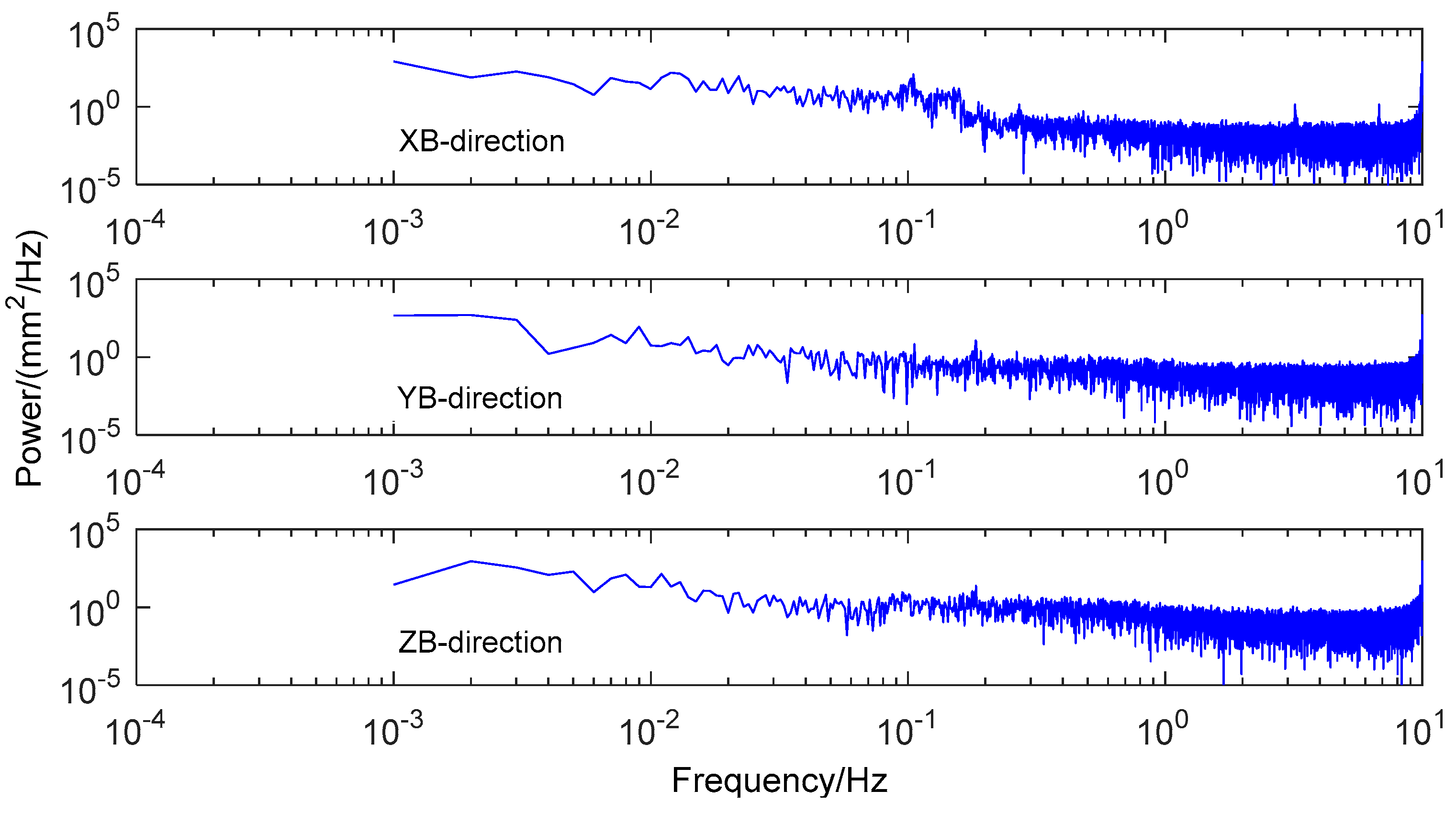
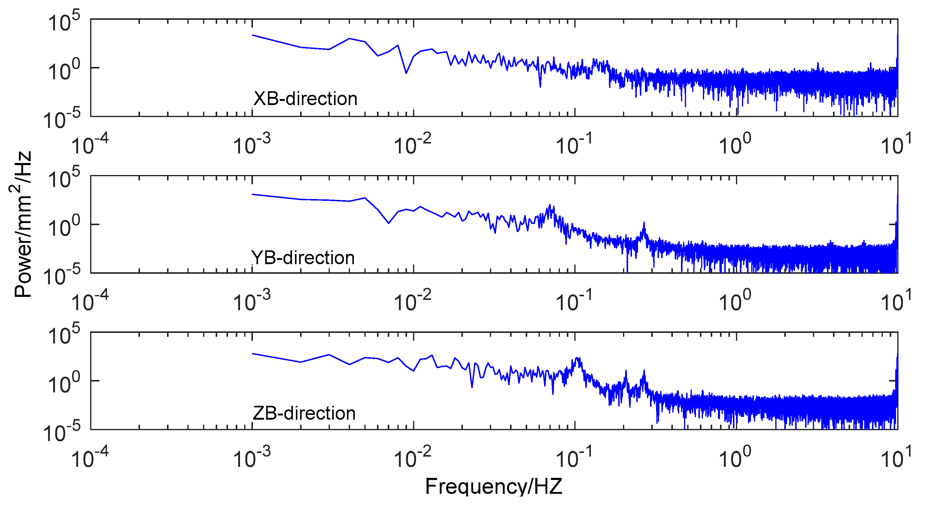
| Station Name | XB (Longitudinal/Hz) | YB (Lateral/Hz) | ZB (Height/Hz) |
|---|---|---|---|
| Shm2 | 0.151 | 0.065 0.268 | 0.105 0.205 0.268 |
| Shm4 | 0.105 0.151 0.183 | 0.183 | 0.183 |
© 2019 by the authors. Licensee MDPI, Basel, Switzerland. This article is an open access article distributed under the terms and conditions of the Creative Commons Attribution (CC BY) license (http://creativecommons.org/licenses/by/4.0/).
Share and Cite
Zhang, Q.; Ma, C.; Meng, X.; Xie, Y.; Psimoulis, P.; Wu, L.; Yue, Q.; Dai, X. Galileo Augmenting GPS Single-Frequency Single-Epoch Precise Positioning with Baseline Constrain for Bridge Dynamic Monitoring. Remote Sens. 2019, 11, 438. https://doi.org/10.3390/rs11040438
Zhang Q, Ma C, Meng X, Xie Y, Psimoulis P, Wu L, Yue Q, Dai X. Galileo Augmenting GPS Single-Frequency Single-Epoch Precise Positioning with Baseline Constrain for Bridge Dynamic Monitoring. Remote Sensing. 2019; 11(4):438. https://doi.org/10.3390/rs11040438
Chicago/Turabian StyleZhang, Qiuzhao, Chun Ma, Xiaolin Meng, Yilin Xie, Panagiotis Psimoulis, Laiyi Wu, Qing Yue, and Xinjun Dai. 2019. "Galileo Augmenting GPS Single-Frequency Single-Epoch Precise Positioning with Baseline Constrain for Bridge Dynamic Monitoring" Remote Sensing 11, no. 4: 438. https://doi.org/10.3390/rs11040438