Radar Interferometry Time Series to Investigate Deformation of Soft Clay Subgrade Settlement—A Case Study of Lungui Highway, China

Abstract
:1. Introduction
2. Methodology
2.1. Linear Deformation Models
2.2. Non-linear SBAS Models
3. Comparison Experiment for Different SBAS-InSAR Deformation Models
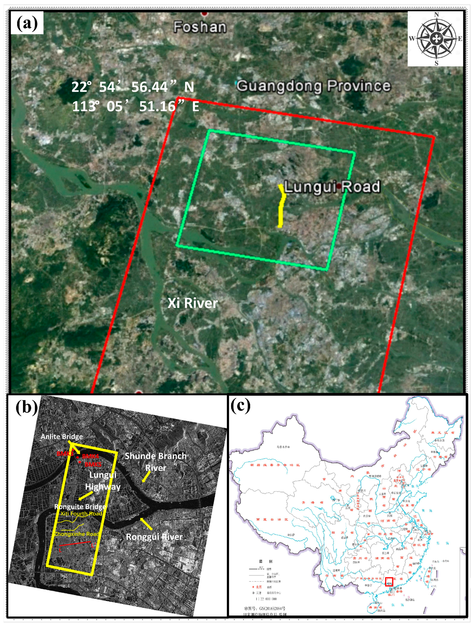
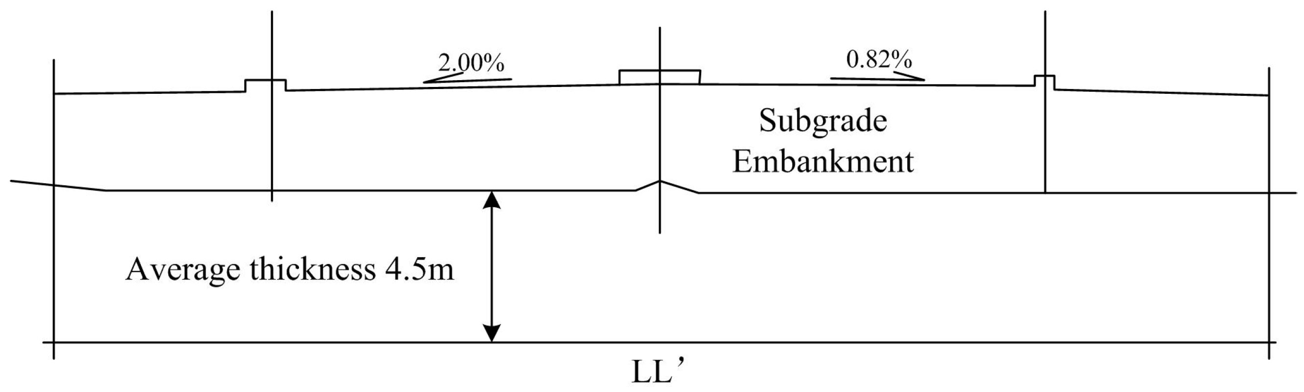
3.1. Study Area
3.2. SAR Acquisitions and Data Processing
3.3. Deformation Parameter Estimation
3.4. Accuracy Assessment of Different SBAS Models
- (1)
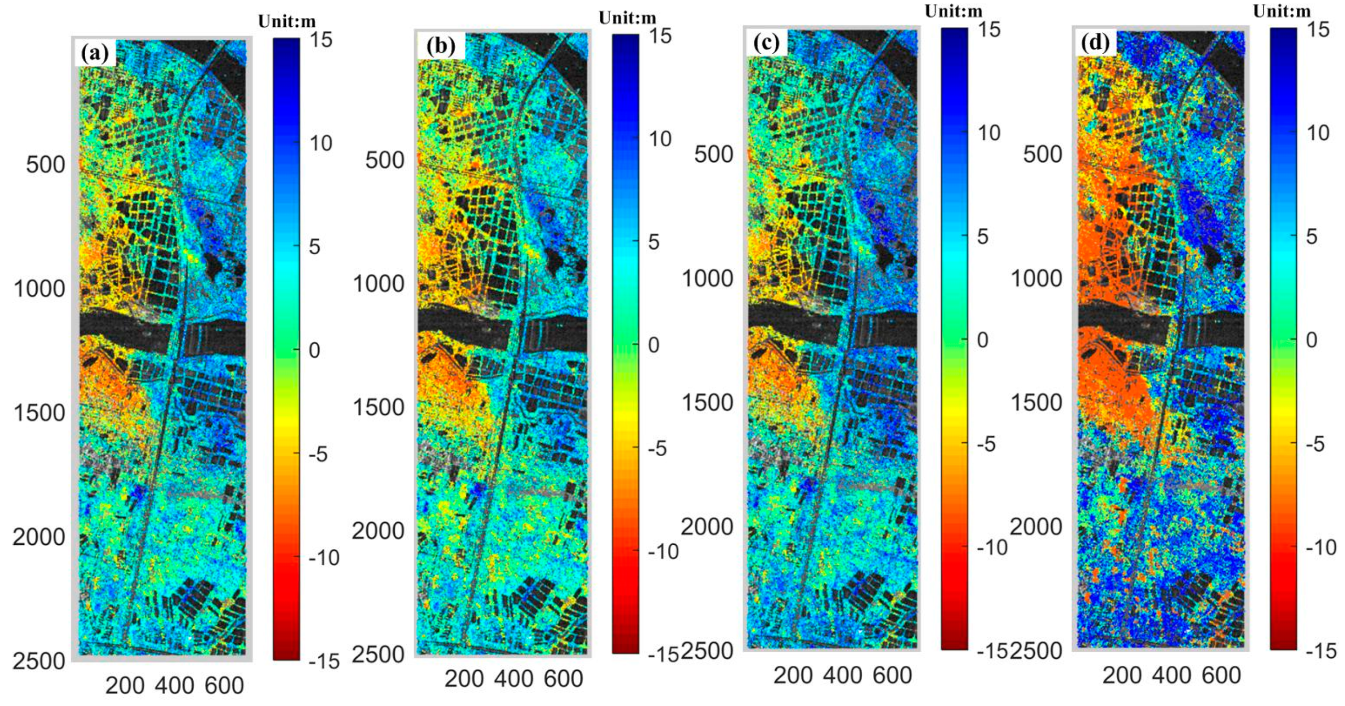
- Residual Phase (RP): in Equation (1), which can be calculated by subtracting the model phase component from the original unwrapped phase observations. This index implies the fitting performance for each model [36]. The smaller the residual phase is, the higher the accuracy for the model selected. RP estimated results are shown in Figure 11. The color bar was set to (−0.5 to 0.5) radians. From the color characteristic in the Figure, we can see that the color for SM distributes around 0.1(mainly light green), for MVM distributes around −0.1 (most light blue), for CPM and PVM both higher than −0.5 (deep blue). Statistically the range of temporal average RP value for the four different models in radians, varied from−0.183 to 0.183, −0.920 to 0.664, −0.157 to 0.188, and −0.811 to 0.660 for LVP, PVM, SM and CPM, respectively. In our case MVM and SM models have better performance.
- (2)
- Temporal Coherence (TC): according to literature [37], was calculated as the temporal mean TC value for different models of all coherent points. A higher TC value defines higher accuracy of the deformation model. From Figure 12, we can find obviously MVM shows the highest TC value (heavy red color all over the total image). PVM has the lightest TC color distribution. The average of TC value for each model is shown in the first row in Table 2, which quantitatively illustrates the performance for the 4 models, consistent with Figure 12.
- (3)
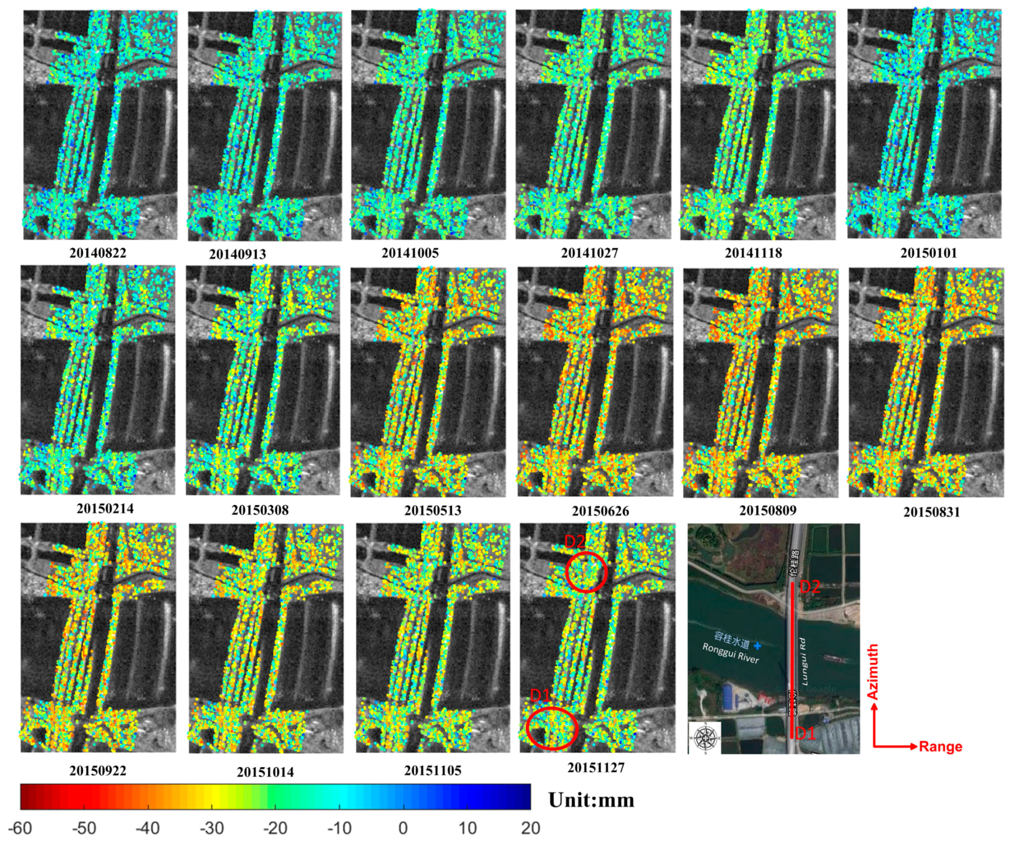
- HP Deformation: according to literature [29], uses the High-Pass (HP) deformation contribution. In Equation (1), the part of is called the Low-Pass (LP) deformation component, which is modelled by the function of deformation coefficients. As all unknowns in the SM model have been estimated, the LP deformation component can be obtained. The atmospheric phase component is highly correlated in space but poorly in time, while the High-Pass deformation signal is highly correlated not only in space but also in time, so the HP-deformation component can be estimated through temporal low-pass filtering (we use triangle filter method here) followed by spatial low-pass filtering (mean filter here) [37]. Figure 13 shows HP deformation between four models on each interferogram. We can see from it that all the HP deformation is lower than 10mm for each interferogram and each model, where the deformation of 10, 12, 13 and 16th interferogram are particular higher. It indicates these 4 interferograms are with larger residual phases. We calculated the Root Mean Square (RMS) value of temporal mean HP deformation for all the high coherent points, which are listed in Table 2.
3.5. Discussion
4. Time Series Deformation Inversion
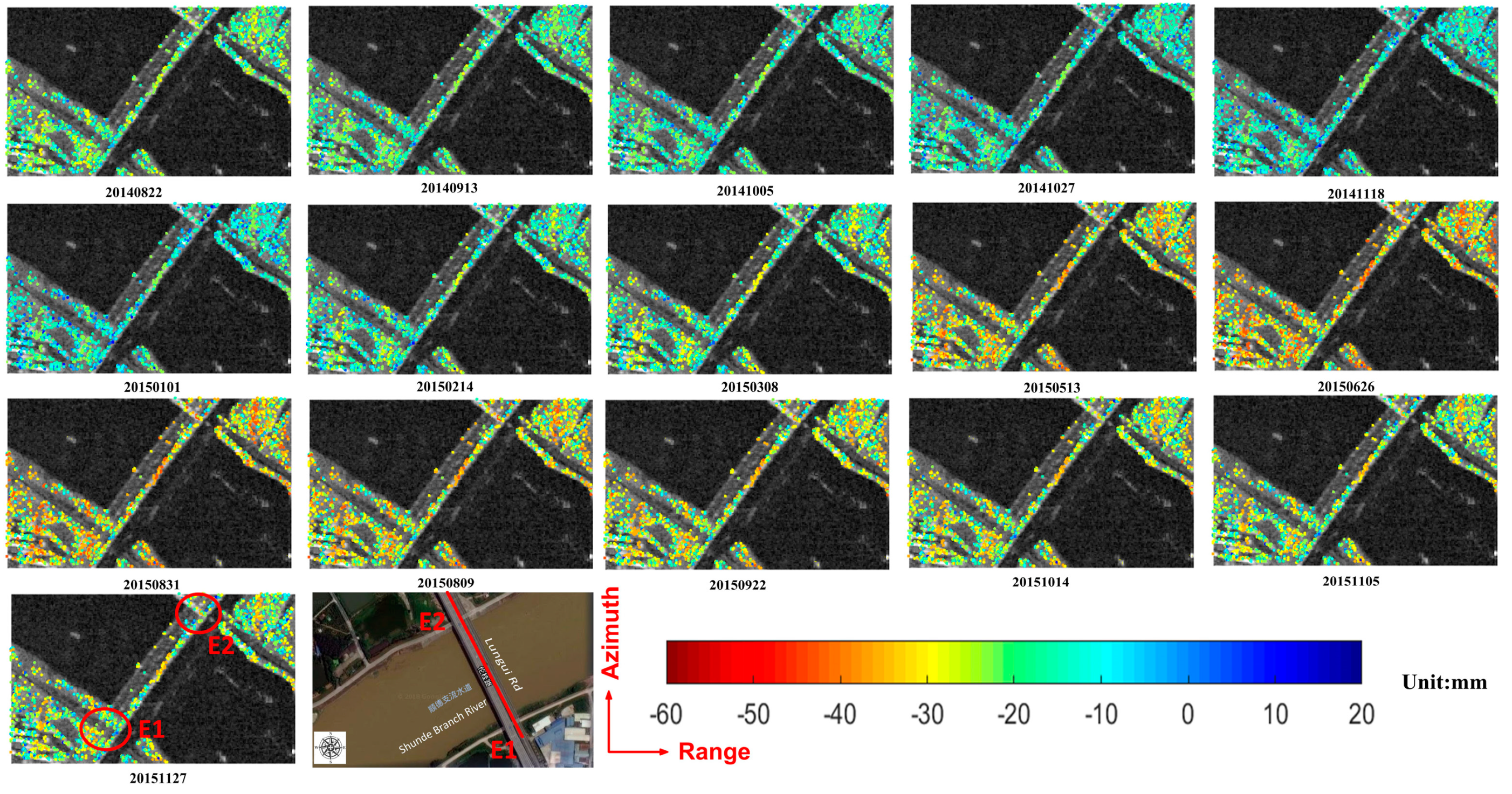
4.1. Overall Characteristics of the Surface Deformation Comparison
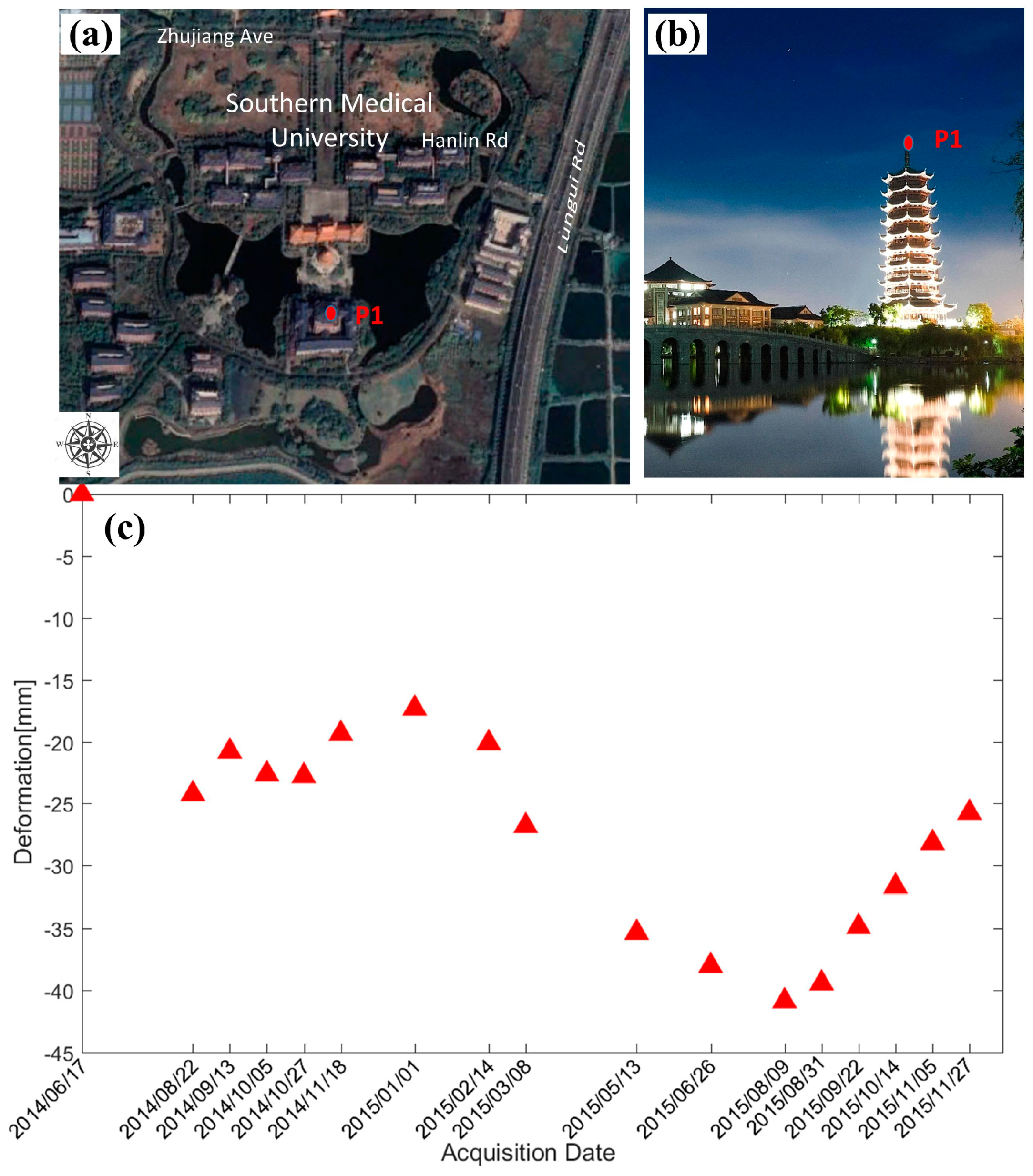
4.2. Deformation over Ground Features-Investigation Based on Seasonal Model
4.2.1. Displacement Characteristics over Two Bridges
4.2.2. Temporal Deformation over Feature Points
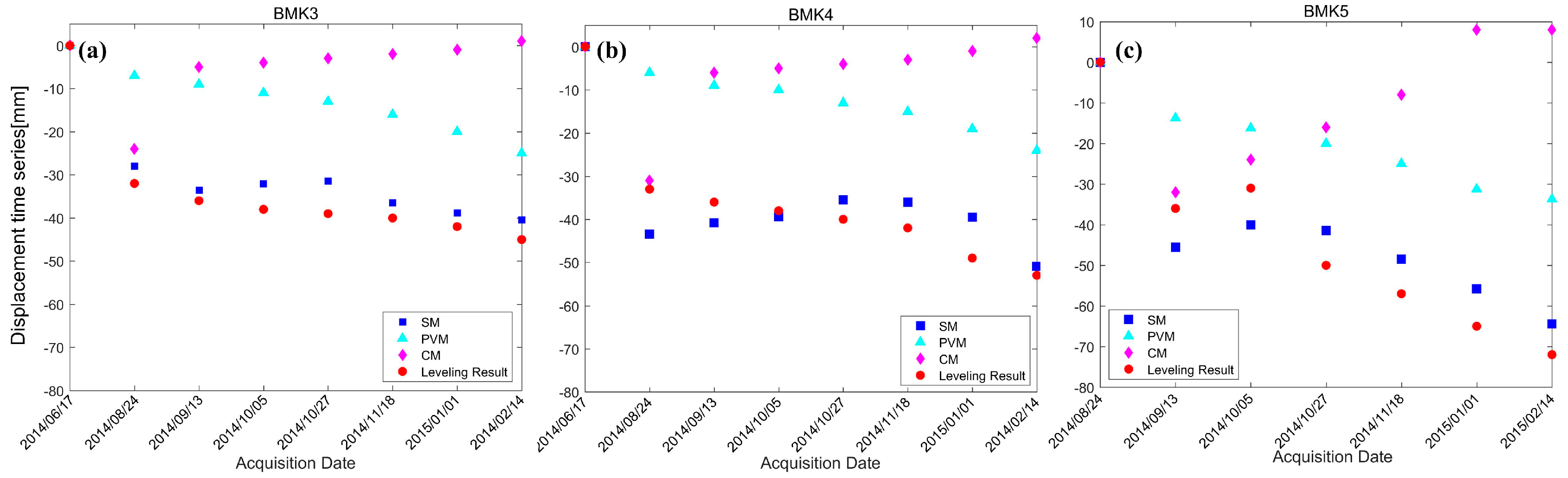
4.3. Comparison with Leveling Measurements
5. Conclusions
Author Contributions
Funding
Acknowledgments
Conflicts of Interest
References
- Zhang, J.; Peng, J.; Zheng, J.; Yao, Y. Characterisation of stress and moisture-dependent resilient behaviour for compacted clays in South China. Road Mater. Pavement Des. 2018, 1–14. [Google Scholar] [CrossRef]
- Zhang, J.; Peng, J.; Zheng, J.; Dai, L.; Yao, Y. Prediction of Resilient Modulus of Compacted Cohesive Soils in South China. Int. J. Geomech. 2018. (online). [Google Scholar]
- Ge, D.Q.; Wang, Y.; Guo, X.; Wang, Y.; Xia, Y. Land subsidence investigation along railway using permanent scatterers SAR interferometry. In Proceedings of the IEEE International Geoscience and Remote Sensing Symposium, Boston, MA, USA, 7–11 July 2008; pp. 1235–1238. [Google Scholar]
- Kobayashi, T. Earthquake rupture properties of the 2016 kumamoto earthquake foreshocks (m j 6.5 and m j 6.4) revealed by conventional and multiple-aperture InSAR. Earth Planets Space 2017, 69, 7. [Google Scholar] [CrossRef]
- Massonnet, D.; Rossi, M.; Carmona, C.; Adragna, F.; Peltzer, G.; Feigl, K.; Rabaute, T. The displacement field of the landers earthquake mapped by radar interferometry. Nature 1993, 364, 138–142. [Google Scholar] [CrossRef]
- Mirzaee, S.; Motagh, M.; Akbari, B. Landslide monitoring using insar time-series and gps observations, case study: Shabkola landslide in northren Iran. Int. Arch. Photogramm. Remote Sens. Spat. Inf. Sci. 2017, 42, 487–492. [Google Scholar] [CrossRef]
- Bayer, B.; Simoni, A.; Schmidt, D.; Bertello, L. Using advanced insar techniques to monitor landslide deformations induced by tunneling in the northern apennines, Italy. Eng. Geol. 2017, 226, 20–32. [Google Scholar] [CrossRef]
- Fan, H.; Gao, X.; Yang, J.; Deng, K.; Yu, Y. Monitoring mining subsidence using a combination of phase-stacking and offset-tracking methods. Remote Sens. 2015, 7, 9166–9183. [Google Scholar] [CrossRef]
- Xing, X.M.; Zhu, J.; Wang, Y.; Yang, Y. Time series ground subsidence inversion in mining area based on CRInSAR and PSInSAR integration. J. Cent. South Univ. 2013, 20, 2498–2509. [Google Scholar] [CrossRef]
- Guardiola-Albert, C.; Herrera, G.; Marchamalo, M.; Ezquerro, P.; TomÃ, R. Mapping groundwater level and aquifer storage variations from insar measurements in the Madrid aquifer, central spain. J. Hydrol. 2017, 547, 678–689. [Google Scholar]
- Hu, B.; Wang, H.-S.; Sun, Y.-L.; Hou, J.-G.; Liang, J. Long-term land subsidence monitoring of Beijing (China) using the small baseline subset (SBAS) technique. Remote Sens. 2014, 6, 3648–3661. [Google Scholar] [CrossRef]
- Hu, X.; Oommen, T.; Lu, Z.; Wang, T.; Kim, J.-W. Consolidation settlement of salt lake county tailings impoundment revealed by time-series InSAR observations from multiple radar satellites. Remote Sens. Environ. 2017, 202, 199–209. [Google Scholar] [CrossRef]
- Jiang, L.; Lin, H. Integrated analysis of SAR interferometric and geological data for investigating long-term reclamation settlement of chek lap kok airport, hong kong. Eng. Geol. 2010, 110, 77–92. [Google Scholar] [CrossRef]
- Hanssen, R.F. Radar Interferometry: Data Interpretation and Error Analysis; Kluwer Academic Publishers: New York, NY, USA, 2001; pp. 188–189. [Google Scholar]
- Hooper, A. A multi-temporal InSAR method incorporating both persistent scatterer and small baseline approaches. Geophys. Res. Lett. 2008, 35, 96–106. [Google Scholar] [CrossRef]
- Ferretti, A.; Prati, C.; Rocca, F. Permanent scatterers in SAR interferometry. IEEE Trans. Geosci. Remote Sens. 2001, 39, 8–20. [Google Scholar] [CrossRef] [Green Version]
- Ferretti, A.; Prati, C.; Rocca, F. Nonlinear subsidence rate estimation using permanent scatterers in differential SAR interferometry. IEEE Trans. Geosci. Remote Sens. 2000, 38, 2202–2212. [Google Scholar] [CrossRef]
- Berardino, P.; Fornaro, G.; Lanari, R.; Sansosti, E. A new algorithm for surface deformation monitoring based on small baseline differential SAR interferograms. EEE Trans. Geosci. Remote Sens. 2002, 40, 2375–2383. [Google Scholar] [CrossRef]
- Mora, O.; Mallorqui, J.J.; Broquetas, A. Linear and nonlinear terrain deformation maps from a reduced set of interferometric SAR images. EEE Trans. Geosci. Remote Sens. 2003, 41, 2243–2253. [Google Scholar] [CrossRef]
- Zhang, L.; Lu, Z.; Ding, X.; Jung, H.-S.; Feng, G.; Lee, C.-W. Mapping ground surface deformation using temporarily coherent point SAR interferometry: Application to LOS Angeles basin. Remote Sens. Environ. 2012, 117, 429–439. [Google Scholar] [CrossRef]
- Dai, K.; Liu, G.; Yu, B.; Deying Ma, H.; Wang, X. Detecting subsidence along a high speed railway by ultrashort baseline TCP-InSAR with high resolution images. In Proceedings of the International Archives of the Photogrammetry, Remote Sensing and Spatial Information Sciences, ISPRS2013-SSG, Antalya, Turkey, 11–17 November 2013. [Google Scholar]
- Yu, B.; Liu, G.; Li, Z.; Zhang, R.; Jia, H.; Wang, X.; Cai, G. Subsidence detection by TerraSAR-X interferometry on a network of natural persistent scatterers and artificial corner reflectors. Comput. Geosci. 2013, 58, 126–136. [Google Scholar] [CrossRef]
- Dong, S.; Samsonov, S.; Yin, H.; Ye, S.; Cao, Y. Time-series analysis of subsidence associated with rapid urbanization in Shanghai, China measured with SBAS InSAR method. Environ. Earth Sci. 2014, 72, 677–691. [Google Scholar] [CrossRef]
- Lazecký, M.; Rapant, P.; Perissin, D.; Bakoň, M. Deformations of highway over undermined Ostrava-Svinov area monitored by InSAR using limited set of SAR images. Procedia Technol. 2014, 16, 414–421. [Google Scholar] [CrossRef]
- Xing, X.M.; Wen, D.; Chang, H.-C.; Chen, L.F.; Yuan, Z.H. Highway deformation monitoring based on an integrated CRInSAR algorithm—Simulation and real data validation. Int. J. Pattern Recognit. Artif. Intell. 2018, 32. [Google Scholar] [CrossRef]
- Hooper, A.; Bekaert, D.; Spaans, K.; Arıkan, M. Recent advances in SAR interferometry time series analysis for measuring crustal deformation. Tectonophysics 2012, 514, 1–13. [Google Scholar] [CrossRef]
- Lin, H.; Ma, P.; Wang, W. Urban infrastructure health monitoring with spaceborne aperture radar interferometry. Acta Geod. Cartogr. Sin. 2017, 46, 1421–1433. [Google Scholar]
- Zhang, Y.; Wu, H.a.; Sun, G. Deformation model of time series interferometric SAR techniques. Acta Geod. Cartogr. Sin. 2012, 41, 864–869. [Google Scholar]
- Armaş, I.; Mendes, D.A.; Popa, R.G.; Gheorghe, M.; Popovici, D. Long-term ground deformation patterns of Bucharest using multi-temporal InSAR and multivariate dynamic analyses: A possible transpressional system? Sci. Rep. 2017, 7, 43762. [Google Scholar] [CrossRef] [PubMed]
- Siles, G.L.; Alcérreca Huerta, J.C.; López Quiroz, P.; Niemeier, W. Long term subsidence analysis and soil fracturing zonation based on InSAR time series modelling in northern zona Metropolitana Del valle De Mexico. Remote Sens. 2015, 7, 6908–6931. [Google Scholar] [CrossRef]
- Li, S.S.; Li, Z.W.; Hu, J.; Sun, Q.; Yu, X.Y. Investigation of the seasonal oscillation of the permafrost over Qinghai-Tibet plateau with SBAS- InSAR algorithm. Chin. J. Geophys. 2013, 56, 1476–1486. [Google Scholar]
- Kampes, B.M.; Hanssen, R.F. Ambiguity resolution for permanent scatterer interferometry. IEEE Trans. Geosci. Remote Sens. 2004, 42, 2446–2453. [Google Scholar] [CrossRef] [Green Version]
- Lauknes, T.R.; Howard, A.Z.; Yngvar, L. InSAR deformation time series using an L1-Norm small-baseline approach. IEEE Trans. Geosci. Remote Sens. 2011, 49, 536–546. [Google Scholar] [CrossRef]
- Yang, Z.; Li, Z.; Zhu, J.; Yi, H.; Hu, J.; Feng, G. Deriving dynamic subsidence of coal mining areas using InSAR and logistic model. Remote Sens. 2017, 9, 125. [Google Scholar] [CrossRef]
- Xing, X.M.; Chang, H.; Chen, L.F. A comparison of time series deformation models based on SBAS-InSAR for soft clay subgrade settlement. In Proceedings of the 2017 Eleventh International Conference on Sensing (ICST), Sydney, Australia, 4–6 December 2017. [Google Scholar]
- Zhao, R.; Li, Z.; Feng, G.; Wang, Q.; Hu, J. Monitoring surface deformation over permafrost with an improved SBAS-InSAR algorithm: With emphasis on climatic factors modeling. Remote Sens. Environ. 2016, 184, 276–287. [Google Scholar] [CrossRef]
- Wang, C.; Zhang, Z.; Zhang, H.; Wu, Q.; Zhang, B.; Tang, Y. Seasonal deformation features on Qinghai-Tibet railway observed using time-series InSAR technique with high-resolution TerraSAR-X images. Remote Sens. Lett. 2017, 8, 1–10. [Google Scholar] [CrossRef]


| Image No. | Acquisition Date (yyyy/mm/dd) | Normal Baseline (m) | Temporal Baseline (Days) |
|---|---|---|---|
| 1 | 2014/06/17 | −71.50 | 198 |
| 2 | 2014/08/22 | −137.97 | 132 |
| 3 | 2014/09/13 | −286.33 | 110 |
| 4 | 2014/10/05 | −110.85 | 88 |
| 5 | 2014/10/27 | −249.06 | 66 |
| 6 | 2014/11/18 | −74.56 | 44 |
| 7 | 2015/01/01 | 0 | 0 |
| 8 | 2015/02/14 | −133.14 | 44 |
| 9 | 2015/03/08 | −106.99 | 66 |
| 10 | 2015/05/13 | −271.51 | 132 |
| 11 | 2015/06/26 | −122.85 | 176 |
| 12 | 2015/08/09 | −149.22 | 220 |
| 13 | 2015/08/31 | −65.63 | 242 |
| 14 | 2015/09/22 | −253.29 | 264 |
| 15 | 2015/10/14 | −159.34 | 286 |
| 16 | 2015/11/05 | −233.83 | 308 |
| 17 | 2015/11/27 | −11.87 | 330 |
| Models | MVM | PVM | SM | CPM |
|---|---|---|---|---|
| Mean Temporal Conference | 0.9320 | 0.6912 | 0.7305 | 0.7158 |
| RMS of HP Deformation (mm) | 1.46 | 2.53 | 1.83 | 2.78 |
© 2019 by the authors. Licensee MDPI, Basel, Switzerland. This article is an open access article distributed under the terms and conditions of the Creative Commons Attribution (CC BY) license (http://creativecommons.org/licenses/by/4.0/).
Share and Cite
Xing, X.; Chang, H.-C.; Chen, L.; Zhang, J.; Yuan, Z.; Shi, Z. Radar Interferometry Time Series to Investigate Deformation of Soft Clay Subgrade Settlement—A Case Study of Lungui Highway, China. Remote Sens. 2019, 11, 429. https://doi.org/10.3390/rs11040429
Xing X, Chang H-C, Chen L, Zhang J, Yuan Z, Shi Z. Radar Interferometry Time Series to Investigate Deformation of Soft Clay Subgrade Settlement—A Case Study of Lungui Highway, China. Remote Sensing. 2019; 11(4):429. https://doi.org/10.3390/rs11040429
Chicago/Turabian StyleXing, Xuemin, Hsing-Chung Chang, Lifu Chen, Junhui Zhang, Zhihui Yuan, and Zhenning Shi. 2019. "Radar Interferometry Time Series to Investigate Deformation of Soft Clay Subgrade Settlement—A Case Study of Lungui Highway, China" Remote Sensing 11, no. 4: 429. https://doi.org/10.3390/rs11040429