Error Analysis on Indoor Localization with Visible Light Communication


1
College of Telecommunications and Information Engineering, Nanjing University of Posts and Telecommunications, Nanjing 210003, China
2
State Key Laboratory of Information Engineering in Surveying, Mapping and Remote Sensing, Wuhan University, Wuhan 430079, China
*
Author to whom correspondence should be addressed.
Remote Sens. 2019, 11(4), 427; https://doi.org/10.3390/rs11040427
Submission received: 21 December 2018
/
Revised: 23 January 2019
/
Accepted: 2 February 2019
/
Published: 19 February 2019
Abstract
:Affected by the complexity of the indoor environment, accurate indoor positioning is challenging in many localization based services (LBS). Recently, it has been recognized that, visible light communication (VLC) is promising for indoor navigation and positioning, due to the low implementation cost with marginal modification to the existing infrastructure and the possibility to achieve high accurate positioning results. Provided that the positions of the light emitting diodes (LEDs) are known to the receiver, the angle of arrival (AOA) of the light signal is able to be estimated by a camera embedded in a smart phone, and thus the position of the smart phone can be derived based on the triangulation. In this paper, the performance of the positioning accuracy is analyzed based on indoor positioning with VLC, and the analytical upper bound of location error is derived. Extensive simulation results have verified the theoretical analysis on the VLC-based localization approach in different indoor scenarios. In order to obtain better location performance, the principles of choosing reference LED and localization LED are also given.
1. Introduction
Since more and more mobile devices are required to exchange data over the wireless channel, the radio spectrum becomes a scarce resource [1,2]. In order to solve this problem, some strategies in efficient usage of the available spectrum have been proposed [3,4,5] and visible light communication (VLC) is one of the most promising solutions [6]. In the last few years, with great advances in solid state electronics, VLC has received significant attention from the research community. As a new paradigm of optical wireless communications (OWC), VLC uses the low-power light-emitting diodes (LEDs) not only for lighting, but also for high data rate downlink communication in homes and offices [7,8,9]. Modern digital communications mostly make use of radio frequency (RF) band, and VLC can address the shortfalls and limitations of RF communications [10].
Recently, the widespread use of LEDs presents a number of opportunities for VLC applications [7,10,11,12,13,14,15,16]. Without requiring any additional hardware in mobile devices, the VLC can provide the location information at a low cost for mobile [8]. Because the LED lighting devices are widely used such as in shopping centers and enterprise markets, additional infrastructure modification to support accurate localization is simpler and cheaper than those for the RF cases. The additional cost would only be some simple programmable logic devices to convey location-related information to mobile devices.
Compared to radio-based positioning, the greatest advantage of VLC-based positioning is that it can almost guarantee the line-of-sight (LOS) condition in the localization area because the LEDs are typically placed on the ceiling and the diffuse component is usually very small relative to the LOS component. Thus, multipath propagation presents less of a challenge than other RF positioning approaches. Meanwhile, LEDs have a number of key advantages in the lifetime, energy saving, quality improvement and environment preservation. Thus, LED-based positioning can be considered as a widely available, cost-effective, and easy-to-use indoor positioning approach. Recently, research interests have increased in this potential indoor positioning technology [17,18]. Ranging methods and techniques with VLC have been proposed for indoor localization, which includes received signal strength (RSS) [19,20], time difference of arrival (TDOA) [21], angle of arrival (AOA) [22] and phase difference of arrival (PDOA) [23]. To be more specific, Ref. [19] takes advantage of the transmitter’s location code at the multiple optical receivers and proposes an LED indoor location estimation algorithm with the RSS measurements. By an additional technique of tilting and the angle-gain compensation process, an improved RSS based VLC positioning approach was also proposed in [20]. Since the path loss of light signal is inversely proportional to the fourth power of the distance [8], which is twice as much as that of the RF signal, the propagation channel parameters limit the accuracy of this kind of localization technique.
In order to avoid the synchronization requirement between the LED panel and receiver, a TDOA technique based VLC positioning method was proposed [21]. By measuring the phase difference between the received signals with respect to one reference LED, the mobile device position can be estimated by linear equations [23]. However, in a short range indoor scenario, both the TDOA technique and PDOA technique can not provide high positioning performance because the time difference/phase difference may be too small to be resolvable due to the high speed of light signals.
In [22], based on the circular-PD-array, an AOA based VLC positioning approach is proposed. In order to improve the positioning performance, both AOA and RSS measurements have been utilized for VLC localization [24]. Because LOS propagation is typically present and a multipath effect is rather marginal, relatively simple optical systems can provide accurate AOA information. Therefore, in this paper, we will focus on this positioning technique. Note that some aspects of the VLC positioning system, such as additional accelerometer measurements [25], hybrid methods [26], protocols [27] and access scheme [28], have also been proposed.
Compared with the plethora of practical algorithms proposed in VLC positioning, the theoretical analysis in this field has not been quite much so far. Among them, the Cramer Rao bound (CRB) on TOA based positioning accuracy is derived in [29], and the CRB is derived for RSS measurements in [30]. In the meanwhile, theoretical analysis on VLC positioning with AOA measurement was limited. It has been noticed that, by exploiting the angle information, VLC positioning with AOA measurements is suitable for practice with respect to implementation cost. Therefore, in this work, we focus on the error analysis on the VLC indoor positioning with AOA measurements. We first present in brief a positioning algorithm proposed in our previous work and then derive the CRB of the algorithm. It has to be mentioned that the error bound can not only provide the performance metrics, but also provide useful information for parameter selection in the algorithm for practical application. In particular, two parameter selection criteria are derived for the position estimation.
The remainder of the paper is organized as follows. The VLC-based indoor positioning model using angle measurements and is described in Section 2. Details of the proposed three-phase positioning approach are presented in Section 2. Section 3 performs the theoretical location error bound analysis. Simulation results are reported in Section 4. Finally, Section 5 draws some conclusions.
2. VLC Indoor Positioning with AOA Measurement
In the considered localization scenario, a number of LEDs are fixed on the ceiling as anchor nodes which are called anchors for simplicity. The anchors regularly transmit encoded light signals so that the receiver can distinguish the signal transmitters. A smart phone receives the LED signal and extracts the angle information from the camera embedded in the smart phone. The position of the receiver is then estimated using the angle information and the known positions of the anchors.
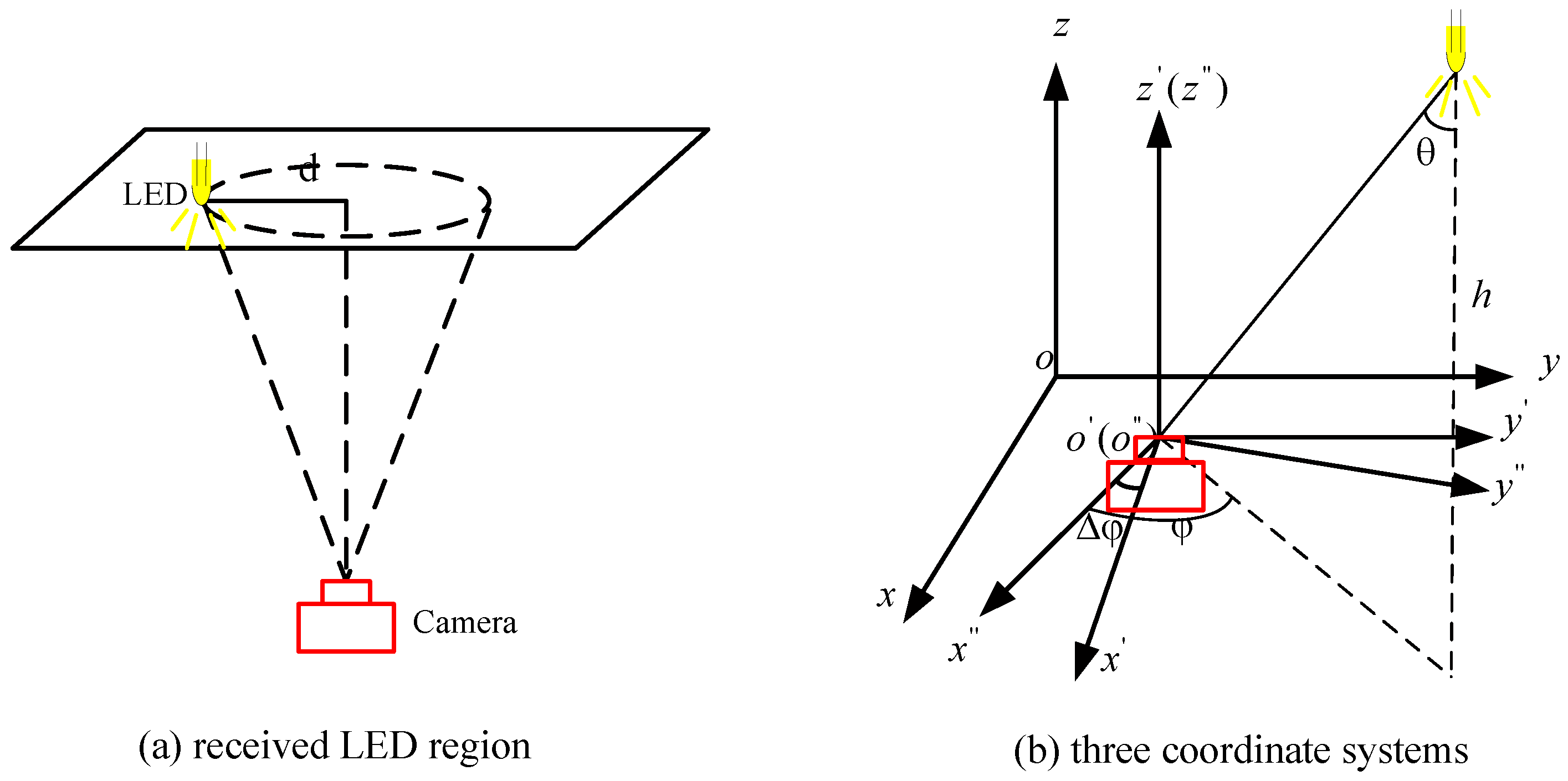
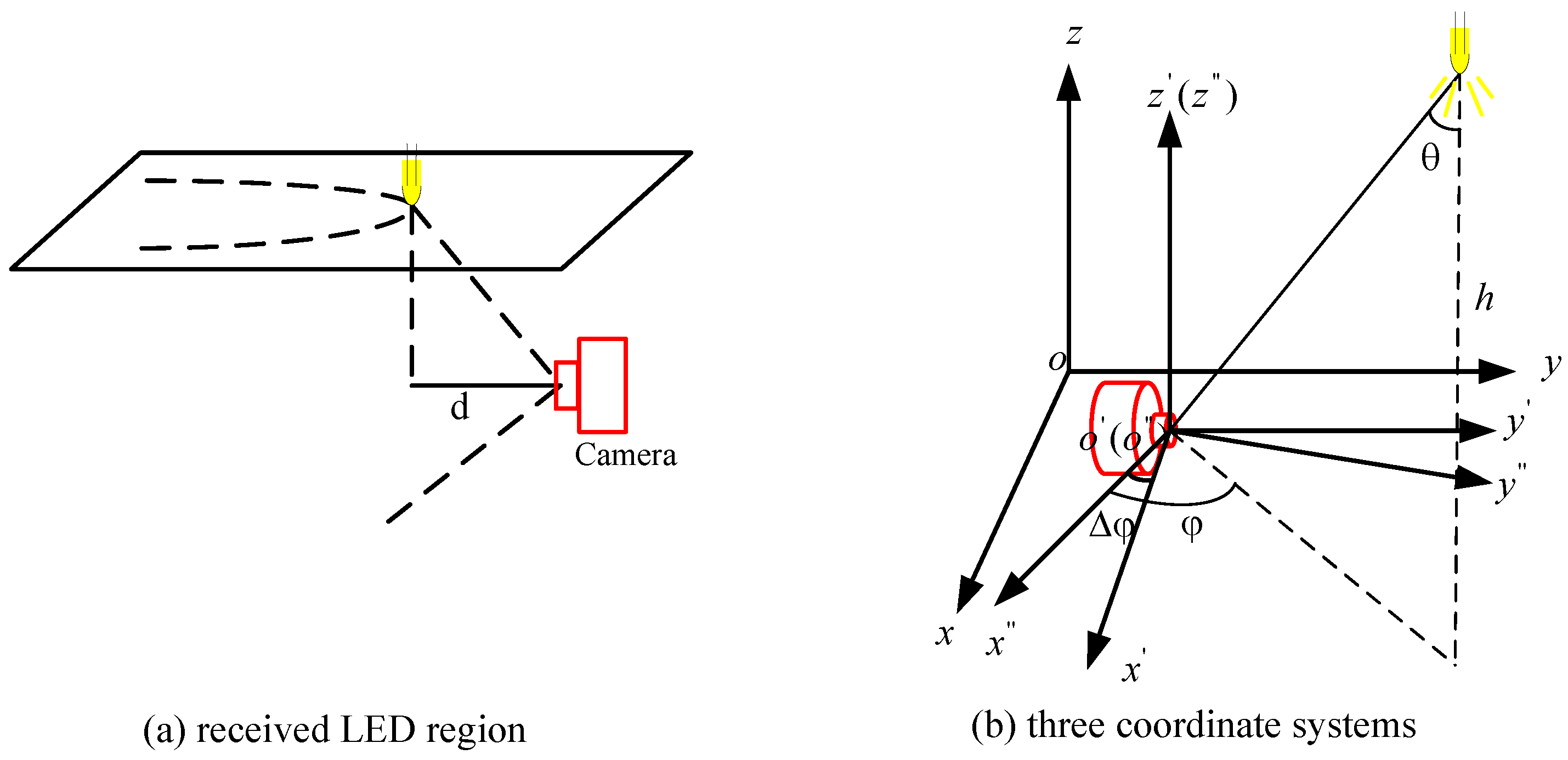
As an example to show the effect of reception mode on the positioning performance, two extreme reception modes are discussed, i.e., the horizontal reception mode and vertical reception mode, which are shown in Figure 1 and Figure 2. When the camera is vertically facing the ceiling, it is defined as the horizontal reception mode. Since the visual angle of the camera is less than , the camera can only see the LEDs within a circle, which is shown in Figure 1a. When the direction of the image sensor is parallel to the ceiling, it is defined as the vertical reception mode. A distinct property of this mode is that it can receive the lights from far LEDs rather than the close LEDs.
In our analysis, three different coordinate systems are defined to simplify the localization problem. The first one is the Absolute coordinate system , which is the pre-defined coordinate system where the positions of all the LEDs are known. The final mobile device position estimates should be given under this coordinate system. The second one is the Shifted coordinate system , which is the shifted or translated version of the absolute coordinate system with the center of the camera (i.e., the mobile device position) as its origin. The third one is the Rotated coordinate system which has the same origin as the shifted coordinate system, i.e., the center of the camera. This third coordinate system would be similar to the camera body coordinate system. The rotation is only around the z-axis so that the -axis and -axis are exactly the same axis for both horizontal and vertical reception modes for analytical convenience. The rotation angle is dependent on the orientation of the camera body. In the case of , the shifted coordinate system and the rotated coordinated system are the same. In the horizontal (vertical) reception mode, the direction of view of the camera is parallel (perpendicular) to the z-axis, -axis, and -axis.
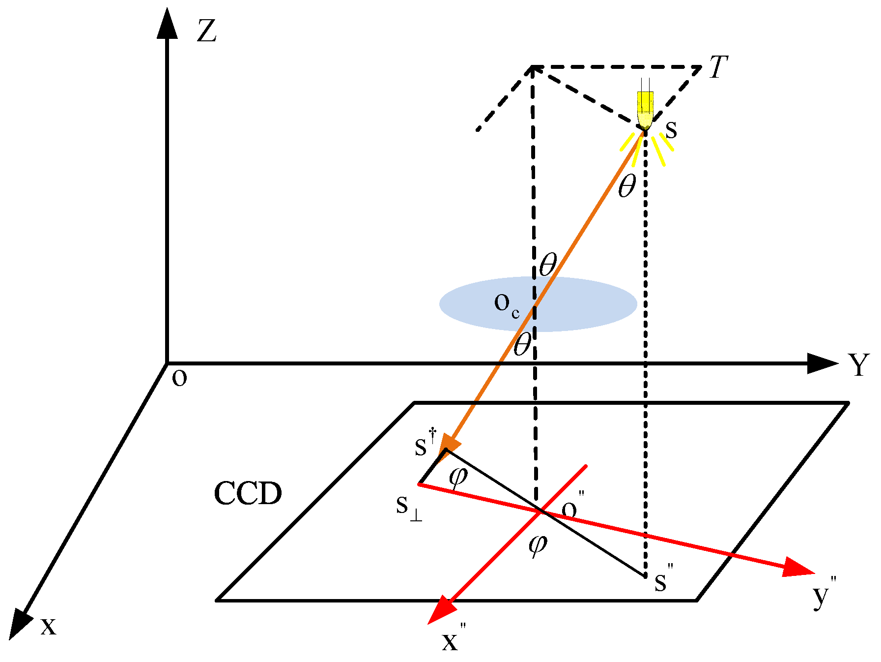
To obtain the angle measurement estimation by the camera, we refer to [31,32]. The geometry for estimation of the polar angle and azimuthal angle based on the imaging of the LED light is illustrated in Figure 3, where and are the center of the Charge-coupled Device (CCD) image sensor and the center of the lens, respectively. Taking the LED with its position s as an example, the project point on the rotated coordinate system is defined as position . The projection point of on the -axis is represented as .
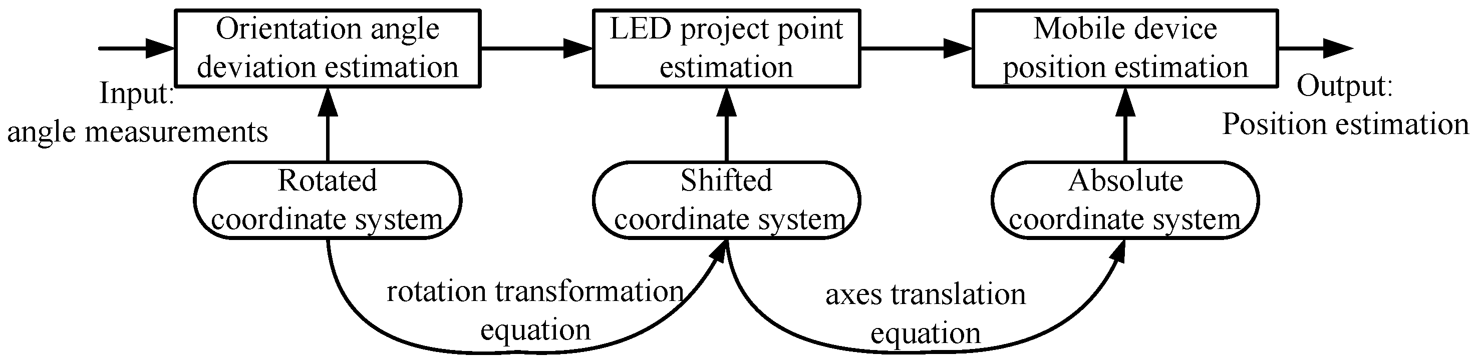
The block diagram of the proposed VLC-based localization scheme for the indoor environment is illustrated in Figure 4. It contains three main phases, namely, the estimation of the orientation angle deviation, LED project point estimation in the shifted coordination system and the final mobile device position estimation. The method was proposed in our previous work [33]; hereby, the three phases are provided in brief as follows.
2.1. Orientation Angle Deviation Estimation
From Figure 1 and Figure 2, the project point of the LED in the rotated coordinate system can be described as:
where , are the polar angle and the azimuthal angle of the LED; h is the height difference between the mobile device and the LEDs which can be calculated as , where and are the height of camera and the LED, respectively.
Since the orientation of the camera body and the shifted coordinate system is usually inconsistent for practical application, the proposed algorithm is concerned with this problem. Assuming the orientation angle deviation is , the project point relationship between the rotated coordinate system and shifted coordinate system associated with the LED can be written as [34]:
where and represent the project points in the rotated coordinate system and the shifted coordinate system, respectively.
Choosing the first LED as a reference LED, we can obtain the following equation by subtracting from [35]
Define , , , , , Then, after some simple mathematical manipulations, Equation (3) becomes
Since the corresponding axes of the absolute coordinate and the shifted coordinate system are parallel, is also the position coordinate shifts in the absolute coordinate system, i.e.,
Define
and
Therefore, the orientation angle deviation can be obtained as
2.2. LED Projection Point Estimation
2.3. Final Mobile Device Position Estimation
Note that the origin of the shifted coordinate system has coordinates in the absolute coordinate system, where are also the coordinates of the mobile device in the absolute coordinate system. The relationship of the LED project point between the shifted coordinate system and the absolute coordinate system can be described as:
where and are, respectively, the LED project position in the shifted coordinate system and absolute coordinate system.
Choosing the LED as the selected localization LED, the final mobile device position can be estimated as:
Note that the localization LED selection rule will also be discussed in the following theoretical analysis section.
3. Theoretical Analysis
3.1. Location Error Analysis
In order to describe the theoretical analysis clearly, we rewrite the rotation matrix as:
where
We define the LED position vector in the shifted coordinate system and rotated coordinate system as
In addition, the measurement noise of polar angle and azimuthal angle are assumed to be and , where and are the associated variance normalized Gaussian random variable, and the constant describes the noise level of the entire system. Note that the measurement noise of polar angle and the orientation angle is assumed to have the same noise level due to the isotropy of the lens.
According to Equation (1), the project vector in the rotated coordinate system can be written as
Assuming that the measurement noise is low, we rewrite Equation (11) by the Taylor expansion formula and obtain
Expanding the terms in Equation (12) and ignoring the higher-order small quantities, Equation (12) becomes
where
According to Equations (5) and (13), the measurement difference vector can be calculated as:
which implies that
and
In the presence of the measurement noise, the orientation angle deviation can be estimated as
The estimated rotation matrix in Equation (9) can be described as
If is small, the matrix inverse can be approximated by [36], we can obtain
In order to calculate the LED project position in the shifted coordinate system, combing Equations (6), (9), (10) and (13), we have Equation (22), which is obtained by ignoring the high order quantity.
Because the true project position of LED in the reference coordinate system can be described as , thus we obtain the estimation error vector from Equation (22) as (23):
Since , where is the identity matrix, is the orthogonal matrix. After the simplification, Equation (23) can be expressed as
Since is the orthogonal matrix, we obtain from Equation (24) that
where represents the maximum eigenvalue calculation. is the 2-norm calculation of matrix A.The inequality is obtained according to the triangle inequality [36].
After some simplification, we reform Equation (25) as (26) where the last inequality is also obtained from [36].
Because , are independent normally distributed random variables with mean 0 and variance 1, statistics , , and follow chi distribution [37]:
As we know, the mean of chi distribution is where k is variance number, is the gamma function. Thus, we can obtain
According to the gamma function definition [38], we have , , , . Thus, Equations (28) and (29) can be simplified as
Therefore, substituting Equations (30) and (31) into (27), we obtain Equation (32). According to Equation (7), we observe that is a shifted version of ; thus, it can be proved that is also the expected discrepancy of the final estimation results. Equation (32) is an important benchmark that reveals which factors will influence the system performance. It will be used in Section 3.2 to help set the system parameters.
3.2. Remarks on the VLC Positioning System
From Equation (32), it can be seen that the reference LED selection ( LED) and the localization LED selection ( LED) have great effects on system performance. There are three observations from Equation (32) which might be useful in system deployment.
- (1)
- Generally speaking, the reference LED ( LED) should be located far away from other LEDs.Assuming all the elements in H are scaled by , (when , the relative distances become larger or vice versa), we obtainThus, when , it can cause the second item of Equation (32) to be larger, therefore resulting in smaller location estimate.
- (2)
- The horizon reception mode can easily produce better position estimation results than the vertical reception mode.First, from the definition of horizon reception and vertical reception mode in Section 2 and Figure 1 and Figure 2, it can be seen that the polar angle of vertical reception model is larger than that of the horizon reception model. In the proposed algorithm, the polar angle is utilized as for position estimation. With the same polar angle deviation , smaller will occur smaller error value, according to the property of the tangent function. Thus, under the same measurement noise scenario, of the horizon reception model is more accurate than that of the vertical reception model because of smaller . Therefore, the positioning performance is better.Next, from Equation (32), it can be found thatTherefore,Thus, it can be concluded that the bound of the final position estimation in the horizon reception mode is also smaller than that of the vertical reception model. If we use the camera to take photo of LED using horizon reception mode and LED using the vertical reception mode, because the polar angle is always smaller than , it is reasonable to assume and . Under this condition, horizon reception mode is easier for obtaining better positioning performance.
- (3)
- The chosen LED for the mobile device location should be the LED closest to the mobile device.From Equation (32), it can be found that the localization LED selection rule reflects the and . When the chosen LED is closer to the mobile device, the will be smaller. From the discussion of Equation (35), the becomes smaller with condition. Therefore, it will decrease the bound of the location error.
4. Simulation Results
4.1. Simulation Setup
In the simulation test, the mobile device is fixed at the position (2 m, 1 m) with the height = 1.5 m. Three LEDs are assumed to be utilized for mobile device localization. Under the same height of LEDs = 4 m, the positions of three LEDs are at three circles with the centre at the position of the mobile device and the radii are 1 m, 2 m and 3 m, respectively. Thus, the height difference h = 2.5 m. Two LED placements are compared to evaluate the localization performance under different conditions. The position information of two placements is described in Table 1. The distances between each LED of two placements are presented in Table 2. According to the position information described in Table 1, the corresponding index of LEDs in different placements are at the same circles, thus the polar angle for ith LED (i = 1, 2, 3) at these two placements is always the same. These simulation environments are designed for special scenario discussion.
4.2. Performance Analysis
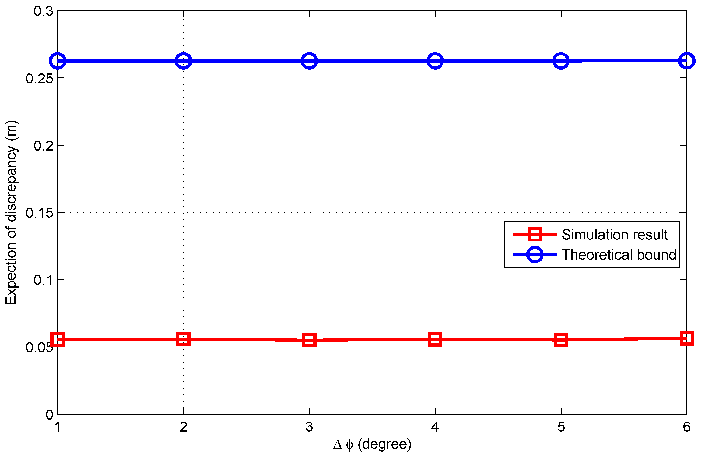
Taking the measurement noise level as (1 degree), Figure 5 illustrated the localization performance and the theoretical bound for the LED placement 2 with different orientation angle deviation , when the first LED is chosen as the reference LED and the localization LED. From the simulation results, it can be seen that the performances are nearly all the same with different s. In addition, it can also be verified by the theoretical bound because the parameter of orientation angle deviation has no effect on the bound of the expectation of the discrepancy.
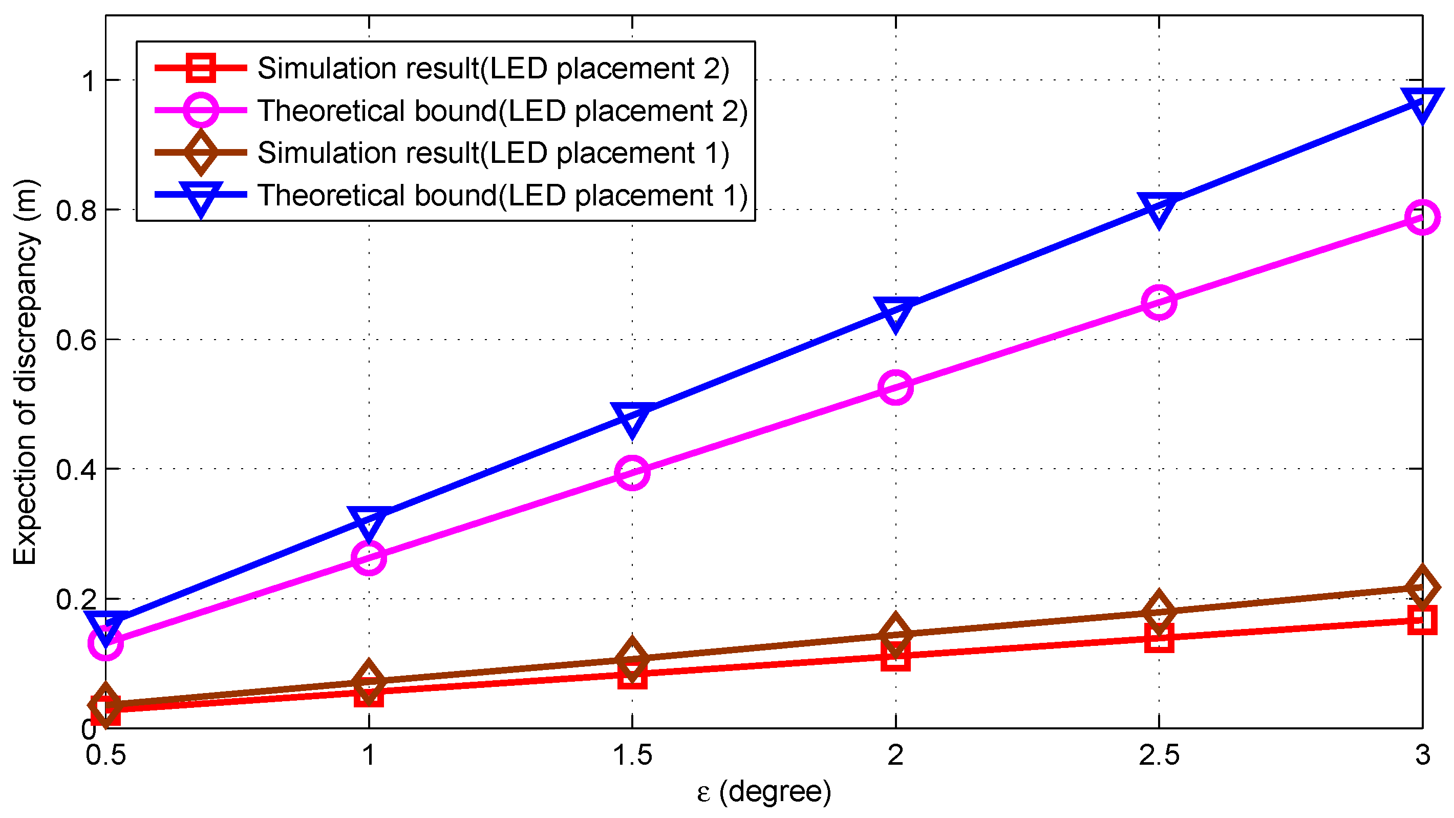
Figure 6 described the simulation results for two different LED placements, when the orientation angle deviation is (two degrees) and the first LED is chosen as the reference LED and the localization LED for final position estimation. As expected, different LED placements have different localization performance. According to the distance information shown in Table 1 and Table 2, under the same chosen LEDs and the polar angle, it can be inferred that the placement with a shorter distance to the reference LED will lead to larger localization error.
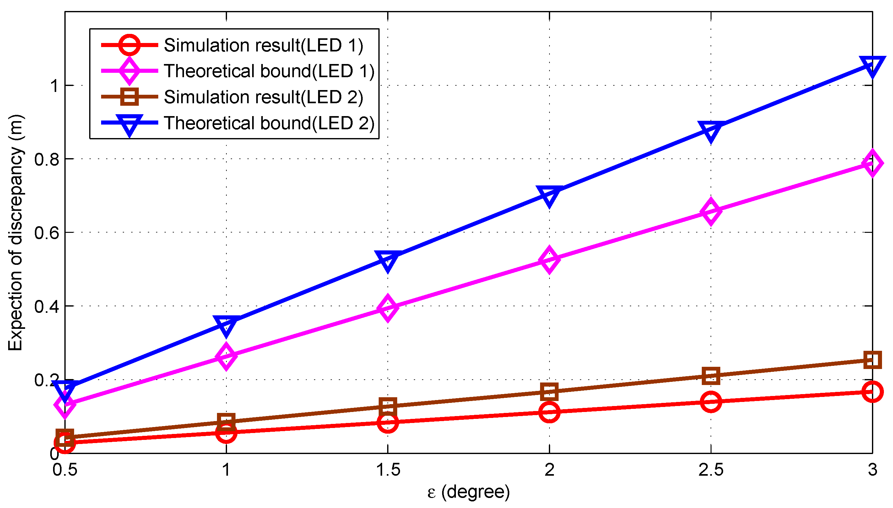
Figure 7 illustrated the performance comparison for different localization LED selection rules, when the reference LED is the first LED. It can be concluded that the proposed algorithm performs better when the first LED is chosen as the localization LED. The theoretical bound is also satisfied with the simulated results. Combining with the simulation results, in this simulation test, under two ith LED selection conditions. However, the 2-norm of the matrix is different. For instance, when the 2-norm for the first LED selection and the second LED selection are and , respectively. Therefore, in order to make better system performance, for localization LED selection, it should make the matrix norm of with a smaller value.
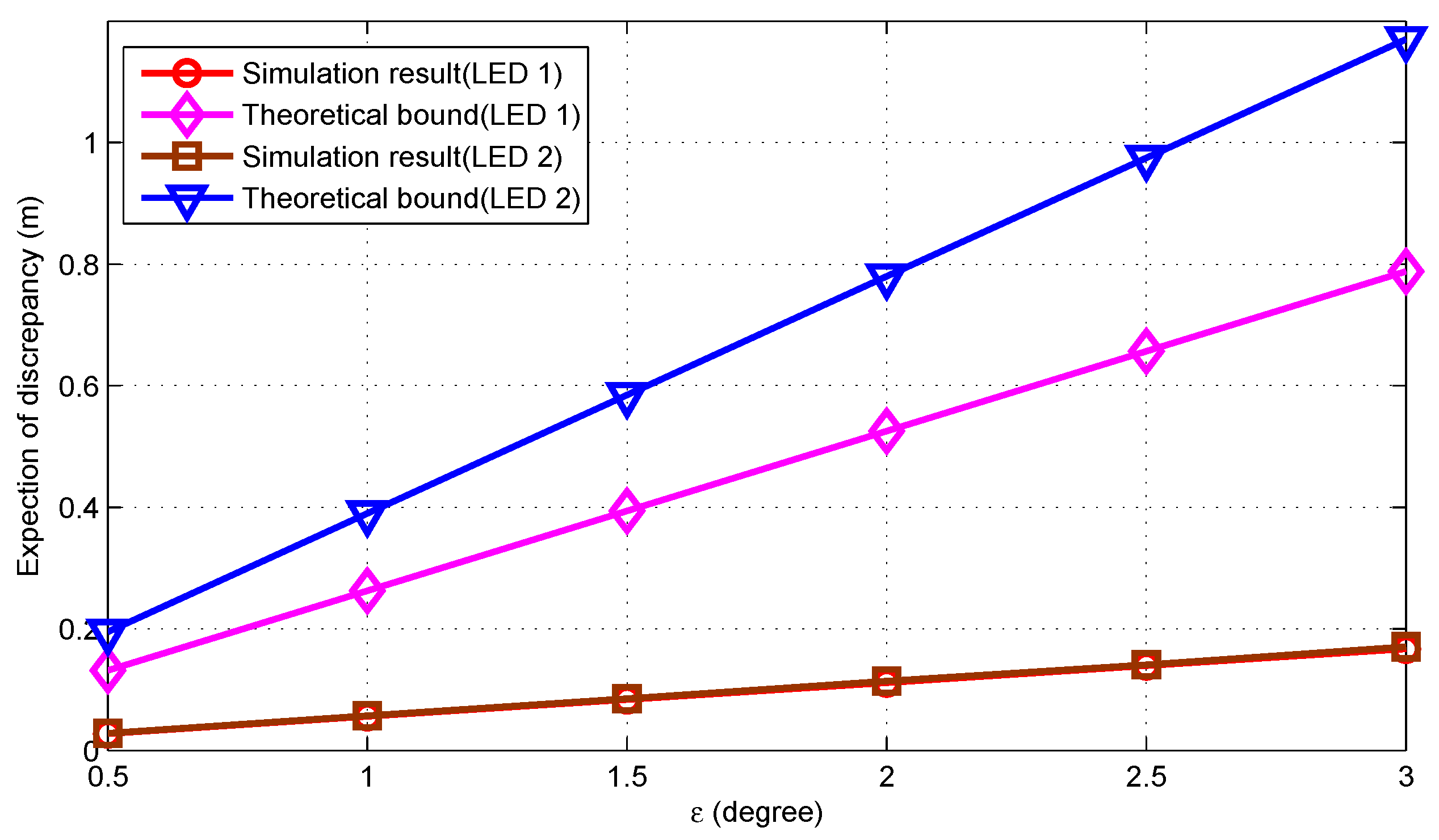
Taking the LED placement 2, the localization LED being the first LED and the orientation angle deviation (2 degree) as an example, Figure 8 shows the performance analysis for different reference LED selection scenarios. From the figure, it can be seen that, when the reference LED is chosen as the second LED, the proposed algorithm performs better. Combining with the prior knowledge, the items of , and in Equation (32) are always the same for these two different conditions. When the reference LED is chosen as the first LED and the second LED and the measurement noise level is , the 2-norm value of the matrix are and , respectively. Thus, in order to make better system performance, for reference LED selection, it also should make the matrix norm of with a smaller value.
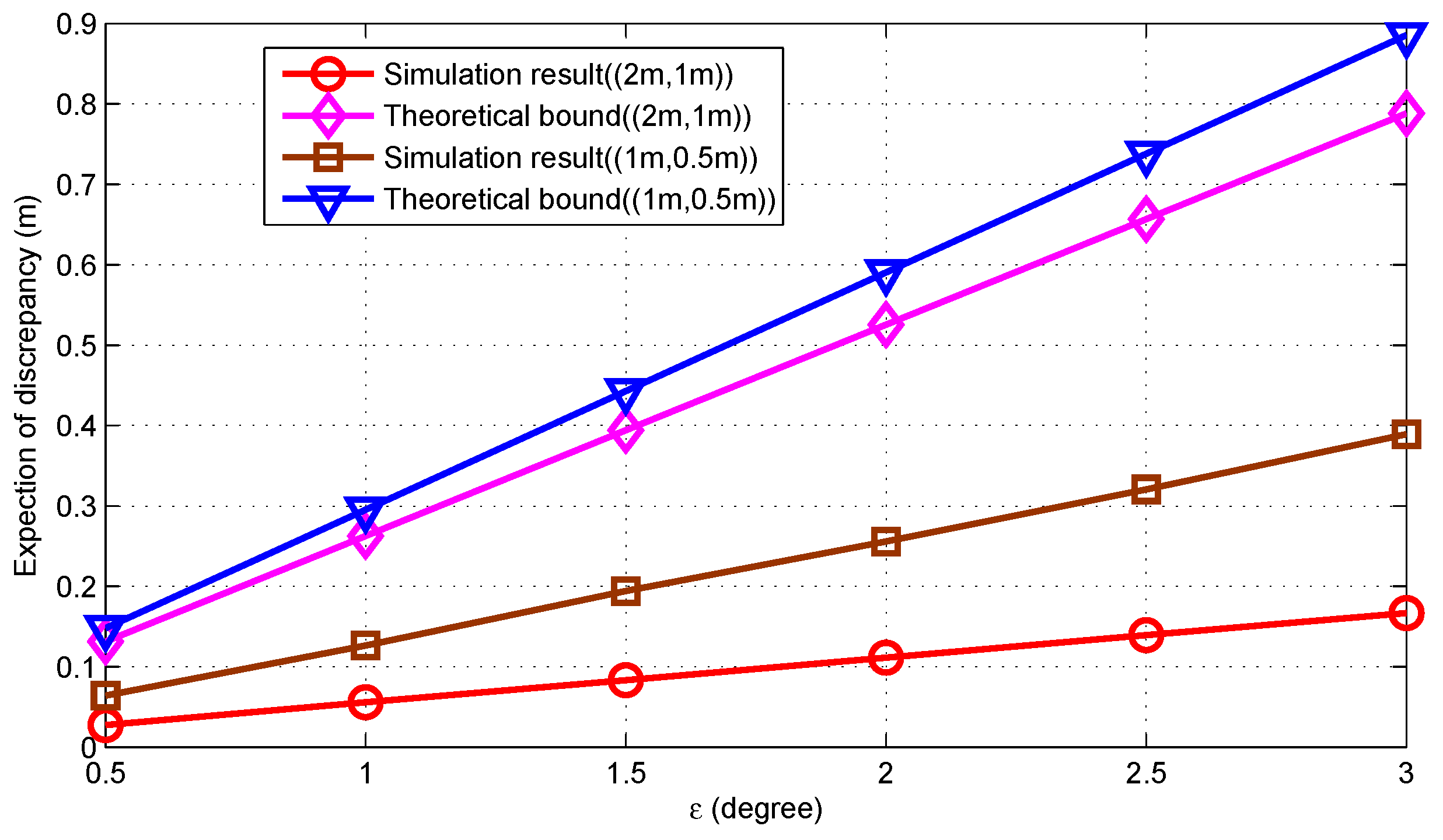
Figure 9 illustrated the performance with LED placement 2, when the mobile device moves from (2 m, 1 m) to (1 m, 0.5 m). In the simulation test, the first LED is chosen as the reference LED and localization LED and the orientation angle deviation (2 degree). It can be seen that, when the mobile device moves away from the LEDs, the localization performance becomes worse. The reason can be explained as follows. When the mobile device is far away from the LED, the polar angle will become larger. Under the same measure noise condition, the deviation of tangent function will change dramatically. Thus, a larger position estimation error will occur.
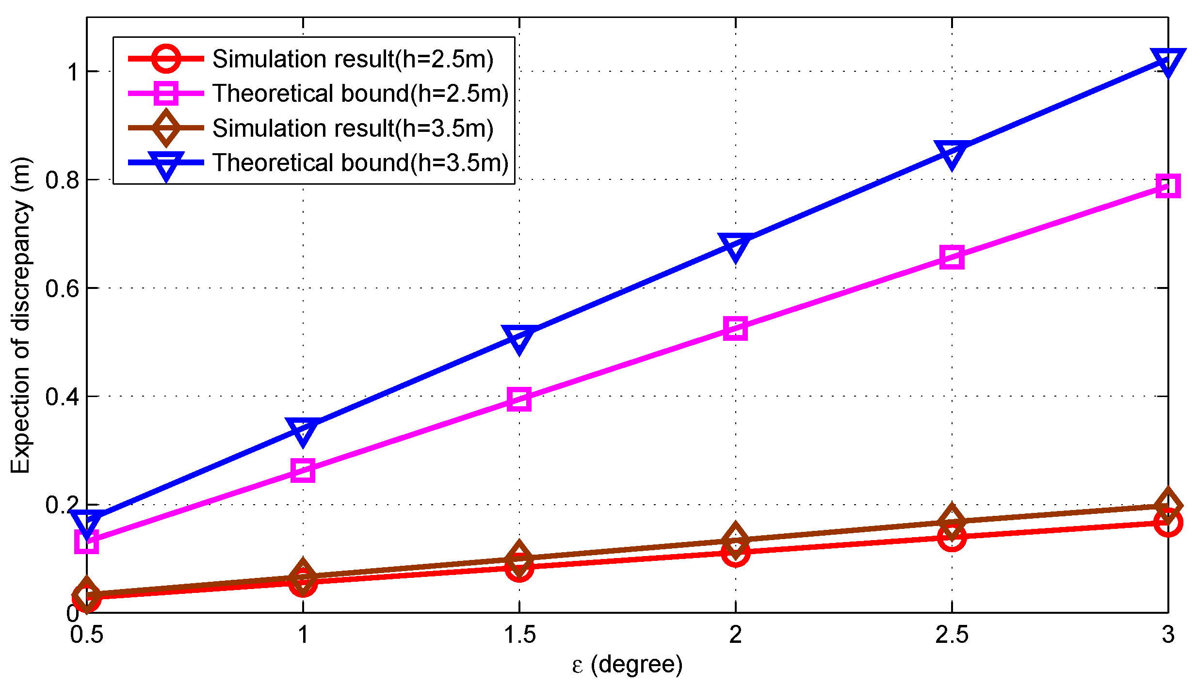
Keeping the height of , the LED placement 2, the reference LED and the localization LED the same, Figure 10 showed the performance analysis with = 5 m and = 4 m, when the orientation angle deviation is (2 degree). In these two conditions, the height differences can be calculated as h = 2.5 m and h = 3 m, respectively. It can be found that both the simulation result and the theoretical bound with smaller height difference have better performance than that of larger height difference. From Equations (13), (14) and (23), it can found that the height difference h is proportional to the parameter. Under the smaller height difference, the final position estimation will become smaller.
5. Conclusions
In this paper, a VLC based localization algorithm is presented at first for mobile device localization in indoor environments. Based on the projection position of LED estimation by the polar angle and azimuth angle measurements, the angle deviation estimation can be obtained using the least square approach. Through the rotation transformation equation, the projection points in the reference coordination system are calculated and the final position estimation can be given by the axes’ translation equation. For another, the upper bound of location error is analyzed to evaluate the theoretical performance and also to optimize the system parameters. In order to obtain better localization performance, the reference LED should be located far away from other LEDs and the chosen LED should be the closest to the mobile device. Simulation results verified the accuracy of theoretical analysis in the VLC-based localization approach under different indoor scenarios. We will continue to study the localization performance in anchor localization error condition. Moreover, similar to the VLC localization technique in [39], a machine learning based VLC localization system is another research topic in the future.
Author Contributions
J.Y., B.Z. and L.C. carried out the theoretical analysis. J.Y., L.C. and J.W. designed experiments and develop the testing tools. J.Y., J.W. and J.L. made the experimental tests and analyzed the data. J.Y., B.Z. and L.C. wrote the manuscript.
Funding
National Natural Science Foundation of China (No. 61771256, 61771258, 61801377), the Project of Innovative Research Team of Hubei Province (Grant no. 2018CFA007) and the Science and Technology Fund of Hubei Province with Project No. 2018AAA070.
Acknowledgments
We thank the suggestive comments from the reviewers.
Conflicts of Interest
There is no conflict interest.
References
- Kenney, J.B. Dedicated short-range communications (DSRC) standards in the United States. Proc. IEEE 2011, 99, 1162–1182. [Google Scholar] [CrossRef]
- Gong, C.; Xu, Z. LMMSE SIMO receiver for short-range non-line-of-sight scattering communication. IEEE Trans. Wireless Commun. 2015, 14, 5338–5349. [Google Scholar] [CrossRef]
- Letaief, K.; Zhang, W. Cooperative communications for cognitive radio networks. Proc. IEEE 2009, 97, 878–893. [Google Scholar] [CrossRef]
- Xin, C.; Song, M. An application-oriented spectrum sharing architecture. IEEE Trans. Wireless Commun. 2015, 14, 2394–2401. [Google Scholar] [CrossRef]
- Han, S.; Liang, Y.; Soong, B.H. Spectrum refarming: A new paradigm of spectrum sharing for cellular networks. IEEE Trans. Commun. 2015, 63, 1895–1906. [Google Scholar] [CrossRef]
- Gavrincea, C.G.; Baranda, J.; Henarejos, P. Rapid prototyping of standard-compliant visible light communications system. IEEE Commun. Mag. 2014, 52, 80–87. [Google Scholar] [CrossRef] [Green Version]
- Yamazato, T.; Takai, I.; Okada, H.; Fujii, T.; Yendo, T.; Arai, S.; Andoh, M.; Harada, T.; Yasutomi, K.; Kagawa, K.; et al. Image-sensor-based visible light communication for automotive applications. IEEE Commun. Mag. 2014, 52, 88–97. [Google Scholar] [CrossRef]
- Jovicic, A.; Li, J.; Richardson, T. Visible light communication: Opportunities, challenges and the path to market. IEEE Commun. Mag. 2013, 51, 26–32. [Google Scholar] [CrossRef]
- Karunatilaka, D.; Zafar, F.; Kalavally, V.; Parthiban, R. LED based indoor visible light communications: State of the art. IEEE Commun. Surv. Tuts. 2015, 17, 1649–1678. [Google Scholar] [CrossRef]
- Wu, S.; Wang, H.; Youn, C. Visible light communications for 5G wireless networking systems: From fixed to mobile communications. IEEE Netw. 2014, 28, 41–45. [Google Scholar] [CrossRef]
- Komine, T.; Nakagawa, M. Integrated system of white LED visible-light communication and power-line communication. IEEE Trans. Consum. Electron. 2003, 49, 71–79. [Google Scholar] [CrossRef]
- Schill, F.; Zimmer, U.R.; Trumpf, J. Visible spectrum optical communication and distance sensing for underwater applications. In Proceedings of the Australasian Conference on Robotics and Automation, Canberra, Australia, 6–8 December 2004; p. 1028. [Google Scholar]
- Hranilovic, S.; Lampe, L.; Hosur, S. Visible light communications: The road to standardization and commercialization (part 1). IEEE Commun. Mag. 2013, 51, 24–25. [Google Scholar] [CrossRef]
- Lim, J. Ubiquitous 3D positioning systems by LED-based visible light communications. IEEE Wireless Commun. 2015, 22, 80–85. [Google Scholar] [CrossRef]
- Wang, J.; Li, H.; Zhang, X.; Wu, R.; Li, H.; Zhang, X.; Wu, R. VLC-based indoor positioning algorithm combined with OFDM and Particle Filter. China Commun. 2019, 16, 86–96. [Google Scholar]
- Lim, S.-K.; Ruling, K.; Kim, I.; Jang, I.S. Entertainment lighting control network standardization to support VLC services. IEEE Commun. Mag. 2013, 51, 42–48. [Google Scholar] [CrossRef]
- Biagi, M.; Pergoloni, S.; Vegni, A.M. LAST: A framework to localize, access, schedule, and transmit in indoor VLC systems. J. Lightw. Technol. 2015, 33, 1872–1887. [Google Scholar] [CrossRef]
- Armstrong, J.; Sekercioglu, Y.A.; Neild, A. Visible light positioning: A roadmap for international standardization. IEEE Commun. Mag. 2013, 51, 68–73. [Google Scholar] [CrossRef]
- Yang, S.H.; Jung, E.M.; Han, S.K. Indoor location estimation based on LED visible light communication using multiple optical receivers. IEEE Commun. Lett. 2013, 17, 1834–1837. [Google Scholar] [CrossRef]
- Yang, S.H.; Jeong, E.M.; Kim, D.R.; Kim, H.S.; Son, Y.H.; Han, S.K. Indoor three-dimensional location estimation based on LED visible light communication. Electron. Lett. 2013, 49, 54–56. [Google Scholar] [CrossRef]
- Do, T.H.; Yoo, M. TDOA-based indoor positioning using visible light. Photon Netw. Commun. 2014, 27, 80–88. [Google Scholar] [CrossRef]
- Lee, S.; Jung, S.Y. Location awareness using angle-of-arrival based circular-PD-array for visible light communication. In Proceedings of the 18th Asia-Pacific Conference on Communications, Jeju Island, Korea, 15–17 October 2012; pp. 480–485. [Google Scholar]
- Nadeem, U.; Hassan, N.U.; Pasha, M.A.; Yuen, C. Highly accurate 3D wireless indoor positioning system using white LED lights. Electron. Lett. 2014, 50, 828–830. [Google Scholar] [CrossRef]
- Yang, S.H.; Kim, H.S.; Son, Y.H.; Han, S.K. Three-dimensional visible light indoor localization using AOA and RSS with multiple optical receivers. J. Lightw. Technol. 2014, 32, 2480–2485. [Google Scholar] [CrossRef]
- Yasir, M.; Ho, S.W.; Vellambi, B.N. Indoor positioning system using visible light and accelerometer. J. Lightw. Technol. 2014, 32, 3306–3316. [Google Scholar] [CrossRef]
- Lee, Y.U.; Kavehrad, M. Two hybrid positioning system design techniques with lighting LEDs and Ad-hoc wireless network. IEEE Trans. Consum. Electron. 2012, 58, 1176–1184. [Google Scholar] [CrossRef]
- Nadeem, U.; Hassan, N.U.; Pasha, M.A.; Yuen, C. Indoor positioning system designs using visible LED lights: Performance comparison of TDM and FDM protocols. Electron. Lett. 2015, 51, 72–74. [Google Scholar] [CrossRef]
- Hou, Y.; Xiao, S.; Zheng, H.; Hu, W. Multiple access scheme based on block encoding time division multiplexing in an indoor positioning system using visible light. J. Opt. Commun. Netw. 2015, 7, 489–495. [Google Scholar] [CrossRef]
- Wang, T.Q.; Sekercioglu, Y.A.; Neild, A.; Armstrong, J. Position accuracy of time-of-arrival based ranging using visible light with application in indoor localization systems. J. Lightw. Technol. 2013, 31, 3302–3308. [Google Scholar] [CrossRef]
- Zhang, X.; Duan, J.; Fu, Y.; Shi, A. Theoretical accuracy analysis of indoor visible light communication positioning system based on received signal strength indicator. J. Lightw. Technol. 2014, 32, 4180–4186. [Google Scholar] [CrossRef]
- Zhu, B.; Cheng, J.; Wang, Y.; Yan, J.; Wang, J. Three-dimensional VLC positioning based on angle difference of arrival with arbitrary tilting angle of receiver. IEEE J. Sel. Areas Commun. 2018, 36, 8–22. [Google Scholar] [CrossRef]
- Sun, X.; Zou, Y.; Duan, J.; Shi, A. The positioning accuracy analysis of AOA-based indoor visible light communication system. In Proceedings of the 2015 International Conference on Optoelectronics and Microelectronics, Changchun, China, 16–18 July 2015; pp. 186–190. [Google Scholar]
- Yan, J.; Zhu, B. A visible light communication indoor localization algorithm in rotated environments. In Proceedings of the 2016 International Conference On Computer, Information and Telecommunication Systems( CITS), Kunming, China, 6–8 July 2016; pp. 1–4. [Google Scholar]
- Leon, S.J. Linear Algebra with Applications; Prentice Hall College Div: Upper Saddle River, NJ, USA, 1999. [Google Scholar]
- Caffery, J.J., Jr. A new approach to the geometry of TOA location. In Proceedings of the IEEE 52nd Vehicular Technology Conference, Boston, MA, USA, 24–28 September 1994; pp. 1943–1949. [Google Scholar]
- Horn, R.A.; Johnson, C.R. Matrix Analysis; Cambridge University Press: Oxford, UK, 1990. [Google Scholar]
- Forbes, C.; Evans, M.; Hastings, N.; Peacock, B. Statistical Distributions, 3rd ed.; Wiley: New York, NY, USA, 2000. [Google Scholar]
- Krantz, S.G. Handbook of Complex Variables; Birkhauser Biston: Boston, MA, USA, 1999. [Google Scholar]
- Alonso-Gonzalez, I.; Rodriguez, D.S.; Ley-Bosch, C.; Suarez, M.A.Q. Discrete indoor three-dimensional localization system based on neural networks using visible light communication. Sensors 2018, 18, 1040. [Google Scholar] [CrossRef]
Figure 1.
Schematic diagram of the horizontal reception mode.

Figure 2.
Schematic diagram of the vertical reception mode.

Figure 3.
Schematic diagram of the angle measurements acquirement.

Figure 4.
Block diagram of the proposed VLC based positioning scheme.

Figure 5.
Performance analysis versus different orientation angle deviations.

Figure 6.
Performance analysis versus different LED placements.

Figure 7.
Performance analysis versus LED selection.

Figure 8.
Performance analysis versus reference LED selection.

Figure 9.
Performance analysis versus mobile device position.

Figure 10.
Performance analysis versus two big differences.


Table 1.
Position of each LED placement.
| LED Placement 1 | LED Placement 2 | |
|---|---|---|
| 1st LED | (3 m, 1 m) | (3 m, 1 m) |
| 2nd LED | (3.93 m, 1.52 m) | (3 m, 2.73 m) |
| 3rd LED | (4.12 m, 3.12 m) | (2.78 m, 3.89 m) |
Table 2.
Distance of each LED placement.
| LED Placement 1 | LED Placement 2 | |
|---|---|---|
| (1st, 2nd) | 1.07 m | 1.73 m |
| (1st, 3rd) | 2.40 m | 2.91 m |
| (2nd, 3rd) | 1.61 m | 1.14 m |
© 2019 by the authors. Licensee MDPI, Basel, Switzerland. This article is an open access article distributed under the terms and conditions of the Creative Commons Attribution (CC BY) license (http://creativecommons.org/licenses/by/4.0/).
Share and Cite
MDPI and ACS Style
Yan, J.; Zhu, B.; Chen, L.; Wang, J.; Liu, J. Error Analysis on Indoor Localization with Visible Light Communication. Remote Sens. 2019, 11, 427. https://doi.org/10.3390/rs11040427
AMA Style
Yan J, Zhu B, Chen L, Wang J, Liu J. Error Analysis on Indoor Localization with Visible Light Communication. Remote Sensing. 2019; 11(4):427. https://doi.org/10.3390/rs11040427
Chicago/Turabian StyleYan, Jun, Bingcheng Zhu, Liang Chen, Jin Wang, and Jingbin Liu. 2019. "Error Analysis on Indoor Localization with Visible Light Communication" Remote Sensing 11, no. 4: 427. https://doi.org/10.3390/rs11040427
Note that from the first issue of 2016, this journal uses article numbers instead of page numbers. See further details here.