Determination of Significant Wave Heights Using Damping Coefficients of Attenuated GNSS SNR Data from Static and Kinematic Observations

Abstract

Currently, GNSS reflectometry based on the signal-to-noise ratio (SNR) has become an established tool in ocean remote sensing. Here, the distance between an antenna and the water surface is measured by analyzing the oscillation of the SNR observation. Due to the antenna gain pattern, this oscillation is more pronounced for satellite signals coming from low elevation angles. Additionally, the sea surface roughness is related to the attenuation of the SNR oscillation. Hence, the significant wave height (SWH) can be estimated by analyzing the SNR signal. In this work, a method is presented with which the SWH can be calculated from the attenuation’s damping coefficient of the SNR observations measured with surface-based receivers. The method’s usability is demonstrated using data from a static antenna operated in the German Bight and with data from a ship-based antenna. The estimated SWH values were validated against numerical wave model data. For both experiments, a high correlation was found.

1. Introduction

The oceans are of major importance for the global climate and life on Earth. In addition to their ecological impact, they play an important role in civil and economic life. Besides knowledge of global and local sea level changes, sea state information is used to gain insights into ocean–atmosphere interaction and is also essential for the planning of coastal protection and shipping safety.

The significant wave height (SWH) is a substantial parameter for describing the sea state in a specific region. This statistical value is defined as the mean value of the highest one-third of wave heights observed over a period of time [1]. A standard technique for doing in situ SWH observations is moored wave buoys where the SWH is calculated from vertical acceleration measurements [1]. Such observations can be used to generate SWH time series for a specific location, which are important for calibration and validation of remote sensing techniques like satellite altimetry [2], marine radar [3], or SAR satellites [4]. Another remote sensing technique is GNSS reflectometry with which a surface is probed using the reflected signal. The SWH can be observed with satellite-based [5] and airborne [6] systems, which make use of the characteristics of delay Doppler maps. For more than a decade, the reflections of GNSS signals have been used for the estimation of sea surface parameters from terrestrial receivers [7]. In particular, during the last few years, the interference of the direct and the reflected signal that creates a characteristic oscillation in the signal-to-noise ratio (SNR), which is observed by the majority of GNSS receivers, has been shown to be a useful tool for observing the distance between a GNSS antenna and the reflecting water surface [8]. Other surface properties like snow coverage [9] or soil moisture [10] can be studied with this method as well. 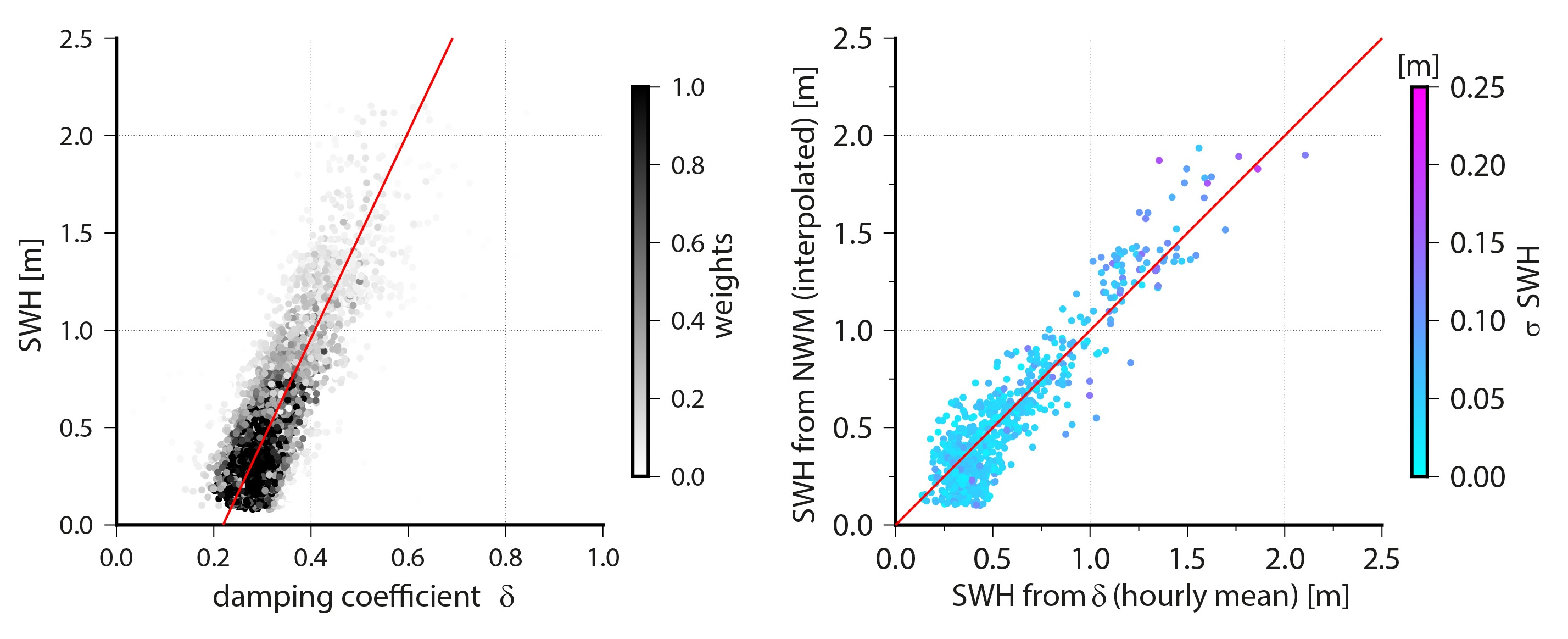The SNR observations also provide the opportunity to make SWH measurements [11]. While a GNSS satellite moves along its orbit, the specular point moves over the water surface, yielding an interference variation with the direct signal, which results in an oscillation of the GNSS SNR observables. The oscillation is attenuated with increasing elevation angles mainly due to the gain pattern of the receiving antenna. Additionally, the attenuation depends on the roughness of the reflecting surface. In Figure 1, SNR observations and the fitted SNR model of two satellites gathered under different wave conditions are presented. The signal gathered at SWH of $1.5$ $\mathrm{m}$ is more attenuated and more noisy than the one gathered at SWH of $0.3$ $\mathrm{m}$. For lower elevation angles, the attenuation due to the antenna gain pattern is commonly low, while an attenuation increase is clearly noticeable when the sea surface is rough.

Alonso-Arroyo et al. used a short-time Fourier transform of the attenuated SNR oscillation to calculate the cutoff angle, at which the signal coherence is lost [11]. They found a non-linear relation between the cutoff angle and the SWH that was observed in parallel by a radar-based instrument. The estimation of higher SWH using this approach is somewhat problematic since the decrease of the cutoff angle is enhanced due to the non-linear structure of the relation. Especially because the influence of tropospheric refraction and shadowing effects grows with low elevation angles, the quality of the SWH could become low.

In this work, we suggest a different approach using the damping coefficient of the attenuated SNR oscillation. Since the attenuation depends exponentially on the damping coefficient, the direct relation between the damping coefficient and the SWH is assumed to show a linear or quasi-linear behavior. We investigated this assumption and its usability using data from two experiments. If the accuracy of the estimated SWH is similar to the accuracy of the wave buoys, these data could be useful for validation purposes. Existing GNSS stations near the coast, on offshore structures, or on ships could be used for such measurements. Especially the possibility of doing SWH observations with GNSS aboard ships could provide useful validation data on the open ocean.

After presenting the methodology in Section 2, the experimental datasets are explained in Section 3. A first experiment was carried out with a one-month dataset from a static antenna. For a second experiment, data from a three-month set of GNSS data, gathered aboard a moving ship, were used. In Section 4, the processing steps to derive the damping coefficient out of an SNR signal are described. Furthermore, antenna-related models of the SWH as a function of the damping coefficient are derived using in situ SWH data from wave buoys. In Section 5, we present a validation of the results using SWH data from an independent wave model. A summary of our findings is given in Section 6.

2. Methodology

According to the full model [12], the SNR is a combination of the direct and reflected power related to the noise power. For a plane reflecting surface, the SNR at time $t_i$ can be decomposed into a trend and interference fringes that are attenuated with respect to the elevation angle:

$$\begin{array}{cc}\hfill SNR& =trend+attenuation·oscillation\hfill \\ \hfill trend& =c_0+c_1{t}_i+c_2{t}_i^2+\cdots +c_n{t}_i^n\hfill \\ \hfill attenuation& =e^{-4k^2{\delta }^2{sin}^2\epsilon },k=\pi /\lambda \hfill \\ \hfill oscillation& =Acos\left(\frac{4\pi }{\lambda }{h}_{ref,t_i}sin\epsilon +{\varphi }_0\right)\hfill \end{array}$$

(1)

Here, the trend is described by a low-order polynomial function of the n unknown parameters c. The attenuation depends on the wave number k, the GNSS signal wavelength $\lambda$, the elevation angle $\epsilon$, and the unknown damping coefficient $\delta$. A and ${\varphi }_0$ are the unknown amplitude and phase offset of the oscillation.

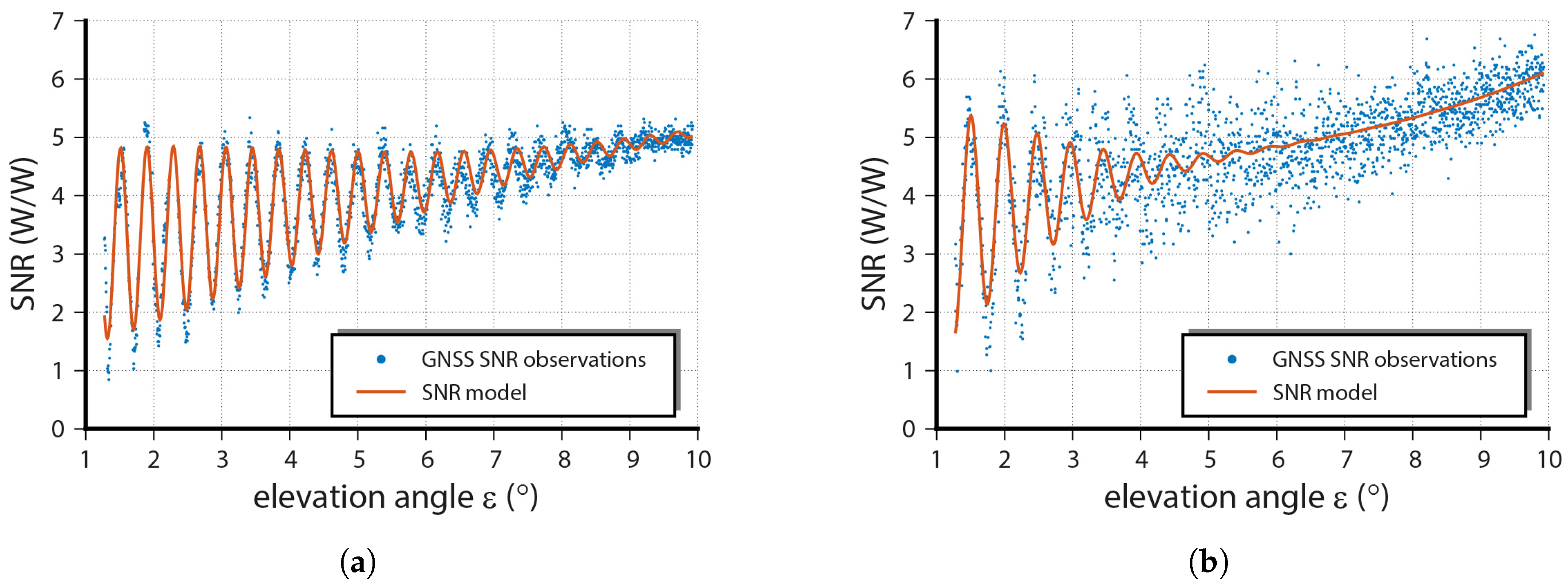
The key parameter describing the oscillation frequency is the reflector height $h_{ref,t_i}$. If this parameter is known, all remaining parameters can be estimated by non-linear least squares estimation for each satellite separately. Therefore, $h_{ref,t_i}$ has to be described as well as possible. In the case of a static antenna, measuring the reflections from a tidally-influenced water surface, this can be done by:

$$h_{ref,t_i}=h_{APC}-h_{gauge,t_i}+d{h}_{sphere,t_i}$$

(2)

The height of the antenna phase center above tide gauge zero $h_{APC}$ can be assumed to be stable for a static antenna. It can either be measured by leveling techniques or estimated using GNSS reflectometry [13]. The tides $h_{gauge}$ cause a height variation with respect to tide gauge zero at epoch $t_i$. If no tidal data are recorded in the vicinity of the measurement site, tidal interpolation may be necessary [14]. Such a procedure will reduce the quality of the correction term and, therefore, the quality of the analysis. In particular, for observations from low elevation angles, the specular point can be several hundred meters away, and a correction $d{h}_{sphere}$ due to the curvature of the spherically-approximated Earth’s surface is required. A simplified geometry is presented in Figure 2a.

For moving antennas, the formula has to be extended for height variations of the antenna. Antennas aboard moving ships are a special case, as the tide-dependent height variations of the water surface can be ignored, but additional hydrodynamic and hydrostatic effects have to be taken into account. The reflector height can be expressed as:

$$h_{ref,t_i}=h_{SRF}-h_{static}+d{h}_{att,t_i}+heav{e}_{t_i}-squa{t}_{UK{C}_{t_i},ST{W}_{t_i}}+d{h}_{sphere,t_i}$$

(3)

Here, $h_{SRF}$ is the antenna height above the ship’s keel. The hydrostatic draft $h_{static}$ can be assumed to be stable for short journeys. For longer journeys, the temporal behavior has to be modeled based on information about the loading condition or from measurements [15]. The hydrodynamic squat is an apparent change of trim and draft while the ship moves through the surrounding water. This effect is caused by the changed pressure conditions around the ship’s hull. The main impact parameters are the shape of the ship’s hull, the under keel clearance (UKC), and the speed at which the ship is moving relative to the water (speed through water (STW)). Speed- and depth-dependent empirical squat models might be applied if available or a method based on GNSS reflectometry can be used [16]. The ship’s attitude $d{h}_{att}$ and heave have an impact on the reflector height and must be taken into account. Both corrections can be obtained by GNSS analysis [16] or from inertial measurement unit (IMU). data [17]. A simplified geometry showing the connection between the parameters in Equation (3) is presented in Figure 2b. In order to keep the illustration simple the parameters $heav{e}_{t_i}$ and $d{h}_{sphere,t_i}$ are not shown.

Since the specular point can be at a substantial distance from the measuring site, the elevation angle will no longer be the complementary angle of incidence. A correction can be calculated according to [16,18]. The elevation angle also has to be corrected for refraction effects. For this, astronomic refraction models can be used [13]. Therefore, the angle $\epsilon$ in Equation (1) must be the elevation angle corrected for both effects.

3. Datasets

3.1. Experiment 1: Static Antenna

The first experiment was carried out with one month of GNSS data gathered from a Leica GR10 receiver and a Leica AR25.R3 antenna during July 2018 (GPS Day of Year 185–216). This equipment is operated by the German Federal Institute of Hydrology (Bundesanstalt für Gewässerkunde (BfG)), and the antenna is installed on a pile atop the tide gauge station TGW2 (Figure 3), which belongs to the German Federal Waterways and Shipping Administration (Wasserstraßen- und Schifffahrtsverwaltung des Bundes (WSV)). The tide gauge is located $1.7$ km north of the coast of Wangerooge island. The sea level is recorded with a 1 min sample rate and a 1 cm resolution. The height offset between tide gauge zero and the antenna reference point is known from BfG information. Depending on the tide, the reflector height above the water surface varies between $10.1$ $\mathrm{m}$ and $14.4$ $\mathrm{m}$. For this experiment, BfG increased the sample frequency of the GNSS receiver to 1 Hz. The antenna’s surroundings are free of static obstacles, and due to the installation structure, negative near-field effects could be assumed to be ruled out. Hence, no azimuth dependent masks were used.

3.2. Experiment 2: Moving Antenna

For the second experiment, data from a moving GNSS receiver were used. This receiver was installed together with two additional receivers aboard of a ferry, which sails from harbors on the German coast to Heligoland island on a daily basis. The installation consists of multiple GNSS Eclipse P307 receivers and Hemisphere A52 antennas. The equipment was installed as part of another project, aiming to measure the sea surface height from moving ships.

Dual-frequency 1 Hz GNSS data were gathered between the beginning of July and the end of September 2017 (GPS Day of Year 186–268). For these 83 days, data from 147 ferry crossings were available for analyses (Figure 4). Due to several restrictions, the antennas had to be installed at the observation deck of the ship’s superstructure. The antenna used for this work was fixed to the forward end of the rail. Hence, an azimuth mask cutting out the superstructure and the mast behind the antenna was used. The GNSS data were routinely analyzed in the frame of the previously-mentioned project. Therefore, the parameters $h_{ref,t_i}$, $h_{static}$, $d{h}_{att,t_i}$, as well as $heav{e}_{t_i}$ from Equation (3) are known. The squat correction was derived from an empirical model estimated previously from a calibration experiment [19].

3.3. Additional Data

3.3.1. Wave Buoys

In the German Bight, sensors measuring the SWH were deployed by federal and scientific institutions, whereby the larger part was installed by the German Federal Maritime and Hydrographic Agency (Bundesamt für Seeschifffahrt und Hydrographie (BSH)). These sensors are either wave buoys or radar sensors. In this work, data from two BSH wave buoys, to the northwest of Heligoland (HelgolandNorthWR) and in the Outer Elbe (ElbeWR) were used. Even if other sensors have higher sampling rates and better resolution properties they were too far away to represent the SWH at the measuring sites. The wave buoys use acceleration data from a 30 min interval to calculate the SWH with a resolution of $0.10$ $\mathrm{m}$. As no accuracy information is provided, a standard deviation of $0.05$ $\mathrm{m}$ had to be assumed.

3.3.2. Numerical Wave Model

The German Weather Service (Deutscher Wetterdienst (DWD)) operates an implementation of the numerical wave model (NWM) WAM [20] for sea state modeling. The modeling setup of the so-called CWAM is especially designed to deal with the conditions in the German coastal regions. The model is driven by the COSMO-DE atmospheric model and the BSH-CMOD water level model from the BSH [21]. CWAM is a purely hydrodynamic model, which is nested into other large-scale models. No in situ observations from wave buoys or other sensors are assimilated. The spatial resolution of this coastal model is about 900 $\mathrm{m}$, and each hour, a SWH parameter set with a resolution of $0.01$ $\mathrm{m}$ is generated. No model accuracy and precision information are provided.

We validated the quality of the model outputs by comparisons with in situ SWH data from three wave buoys using data from the year 2017. The buoys were located in deep and shallow water areas to study the model performance under different conditions. The validation results are summarized in

Table 1. Comparison statistics between the numerical wave model and wave buoy observations at three different sites.

Buoy Name	Latitude ${}^{\circ }$	Longitude ${}^{\circ }$	Water Depth m	Mean Difference m	RMS m	Correlation %
HelgolandNorthWR	54°13.164′	7°49.109′	26	0.027	0.207	97
ElbeWR	53°59.825′	8°06.630′	25	−0.002	0.202	97
BunkerHill	54°47.500′	8°16.300′	6	0.014	0.148	96

. All three validation sites showed no systematic offsets and similar root mean square (RMS) values of up to $0.21$ $\mathrm{m}$. Therefore, it was assumed that the model quality was good enough to validate the functional models that will be calculated in Section 4.

4. Processing and Modeling

Besides the roughness of the reflecting surface, the attenuation of the SNR data is governed by the antenna gain pattern. For antennas of the same type, the gain patterns can be assumed to be similar, whereas it is commonly different for different antenna types. Hence, if SWH is described as a function of the damping coefficient of the attenuation, individual models must be constructed for every antenna type. For that purpose, we used the SNR data from both experiments and calculated the damping coefficient according to Equation (1) in conjunction with either Equation (2) or (3). Later, we used in situ SWH data from buoys to find individual describing functions.

For all datasets, we split the satellite tracks into descending and ascending arcs with elevations above 1° and below 10°. Observations from lower elevation angles were too noisy for evaluation. The higher elevation limit was chosen due to the antenna gain pattern in the case of the static antenna, while in the case of the ship’s measurement, the specular point had to lay outside of the ship’s wave system [16]. The elevation angles were corrected for tropospheric refraction using the refraction model of [22]. The required pressure and temperature data were taken from DWD weather stations at Alte Weser Lighthouse and on Heligoland.

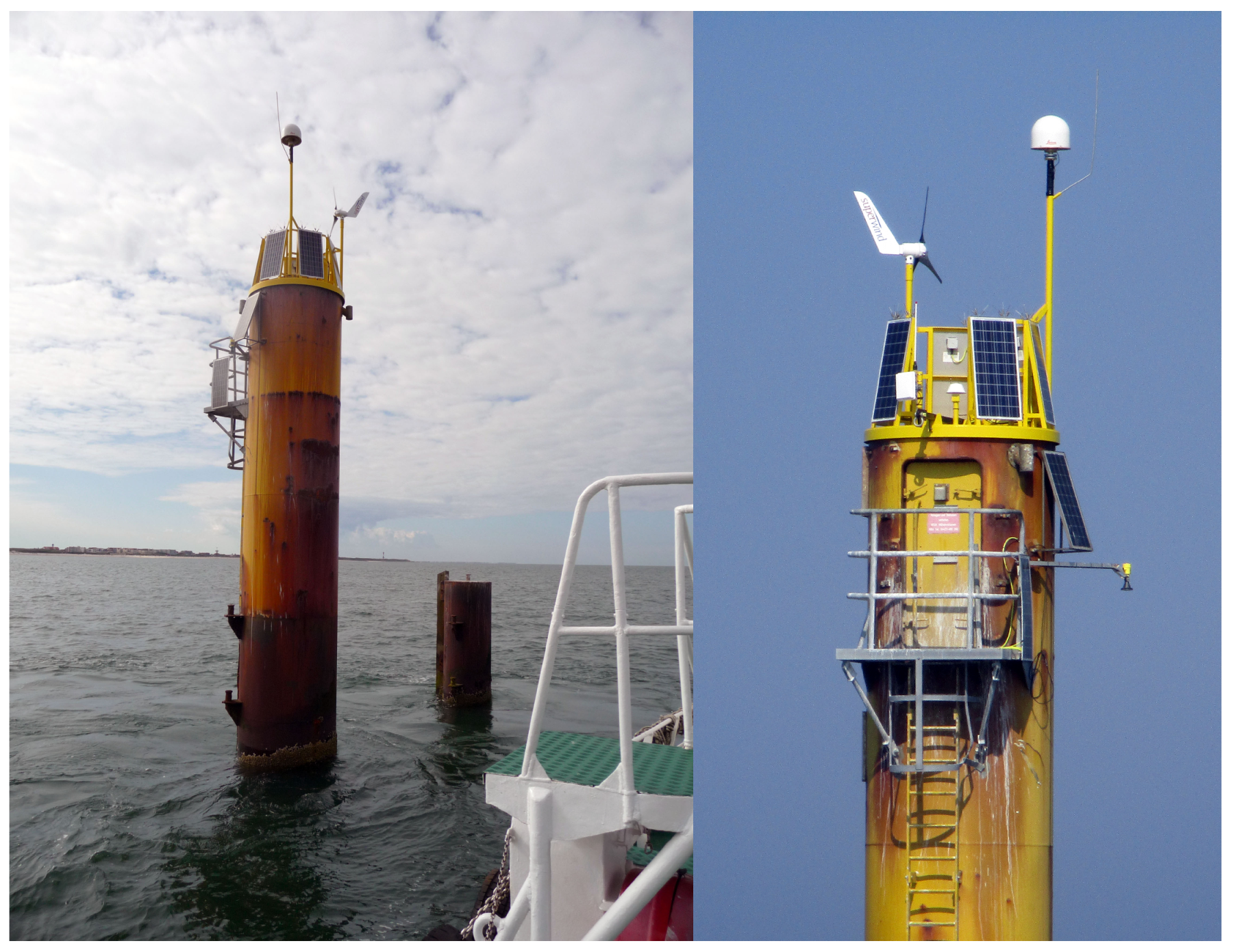
The first experiment was done under ideal circumstances as the GNSS antenna was installed directly above a tide gauge station. Therefore, the tide gauge readings could be directly used to generate the height variation correction $h_{gauge}$. The estimation of the unknown damping coefficient $\delta$, amplitude, and phase, as well as of the unknown trend function parameters was done for each GPS and GLONASS satellite separately. To ensure a sufficient amount of data for a reliable parameter estimation, only arcs with elevation angles ranges of more than 3° were analyzed. The estimation was carried out as a non-linear least squares adjustment. We solved the optimization problem by applying the Levenberg–Marquardt algorithm to avoid divergence due to insufficient initial values for the damping coefficients.

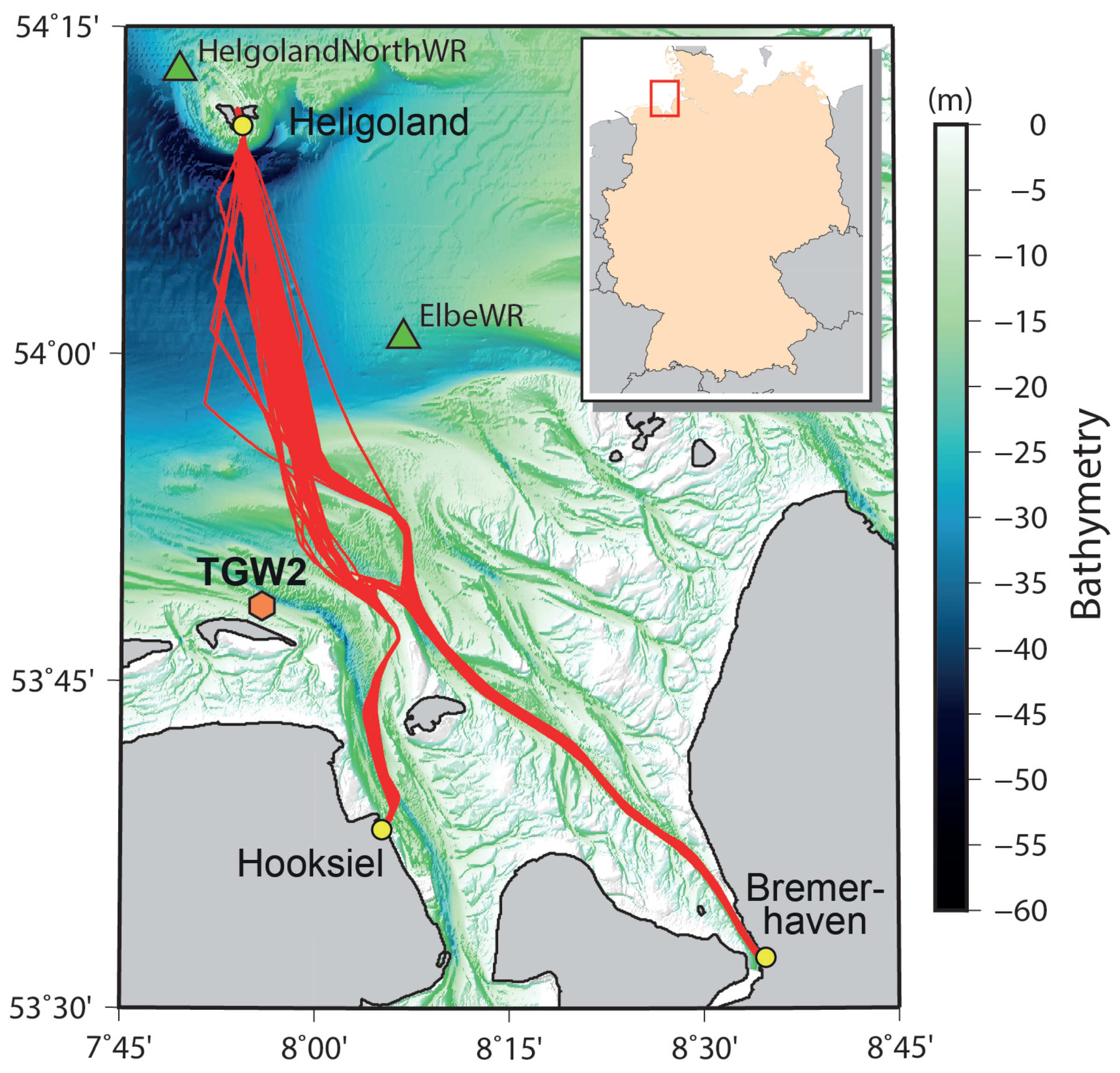
The reference SWH values were interpolated from ElbeWR wave buoy data. The reference epochs for interpolation were set as the mid epochs of the satellite arcs. Due to data gaps at the wave buoy, epochs with a time gap of larger than 30 min to the next buoy measurement epoch had to be excluded. Since the distance between the tide gauge station and the ElbeWR buoy is about 24 km, a correction was required. For that, the SWH from the NWM at both the position of the buoy and the tide gauge was calculated. The difference between the resulting values was used as a correction term. Because of the buoy observation resolution and the model uncertainty, the corrected SWH could become negative during low wave heights. Two percent of the corrected SWH were negative. To avoid such unrealistic values, the minimal SWH was set to $0.1$ $\mathrm{m}$, taking into account the data resolution. In total, 6193 (3528 GPS/2665 GLONASS) satellite arcs could be processed.

In the second experiment, the 83 days of ship tracks were split into segments of deep or shallow water, while a water depth threshold of 25 $\mathrm{m}$ was assumed. This distinction is useful since, for the ship used here, the squat does only depend on the easy-to-observe speed when the water is deeper than 25 $\mathrm{m}$. As a consequence, the quality of the calculated squat can be assumed to be better. In total, 323 segments were found, from which 127 were in deep water and 196 in shallow water regions. Shallow water segments were used only for validation in Section 5. The estimation of a SWH model as a function of $\delta$ was carried out with data from deep water segments only.

The SNR data were analyzed in the same way as for the first experiment, whereby the correction terms in Equation (3) were taken from the GNSS processing in the other project mentioned above. The usable segments had an average length of ca. 40 min twice a day. Due to this fact and, additionally, due to the necessary azimuth mask, the number of analyzed satellite arcs was only 633 (362 GPS/271 GLONASS). The required SWH values at the ship’s position were spatially interpolated from the wave buoy data. Unlike the first experiment, no SWH correction had to be used.

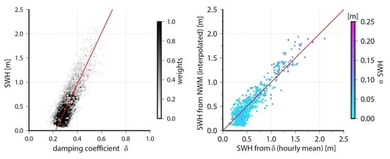
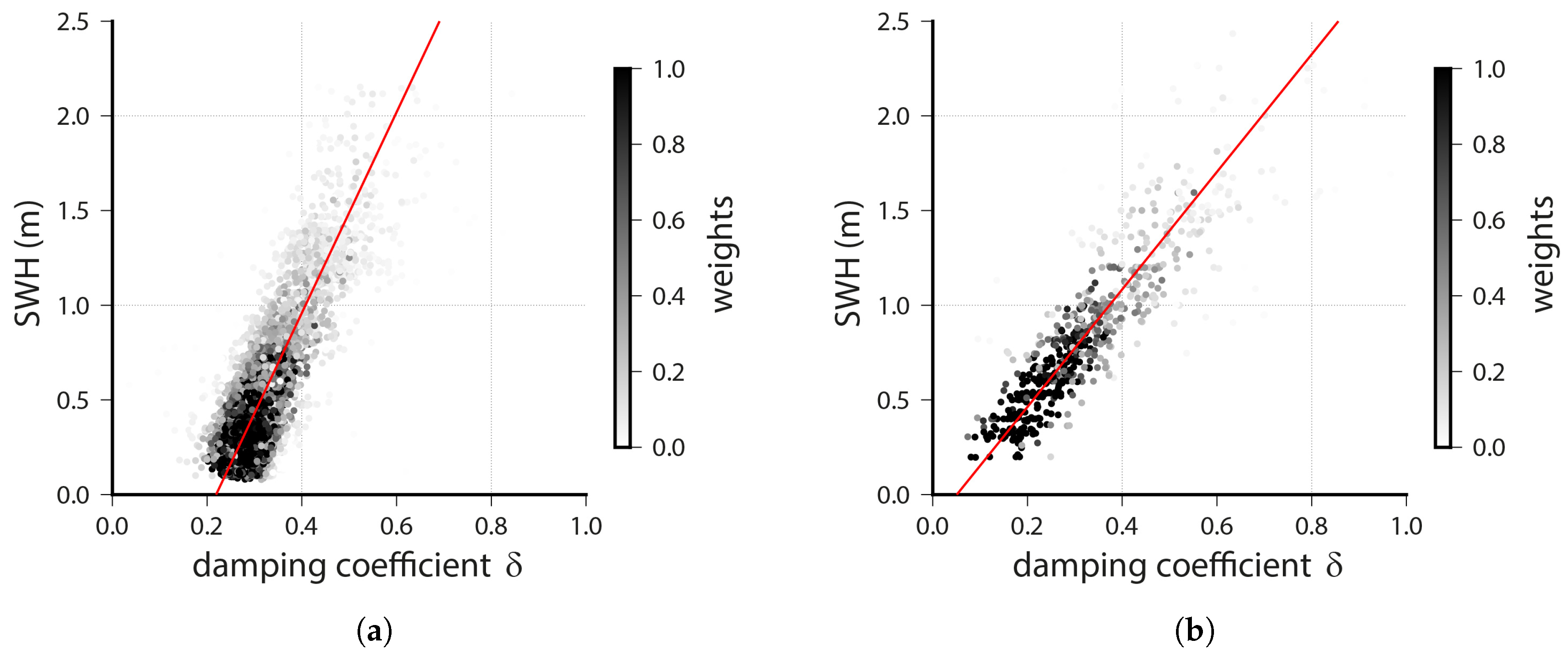
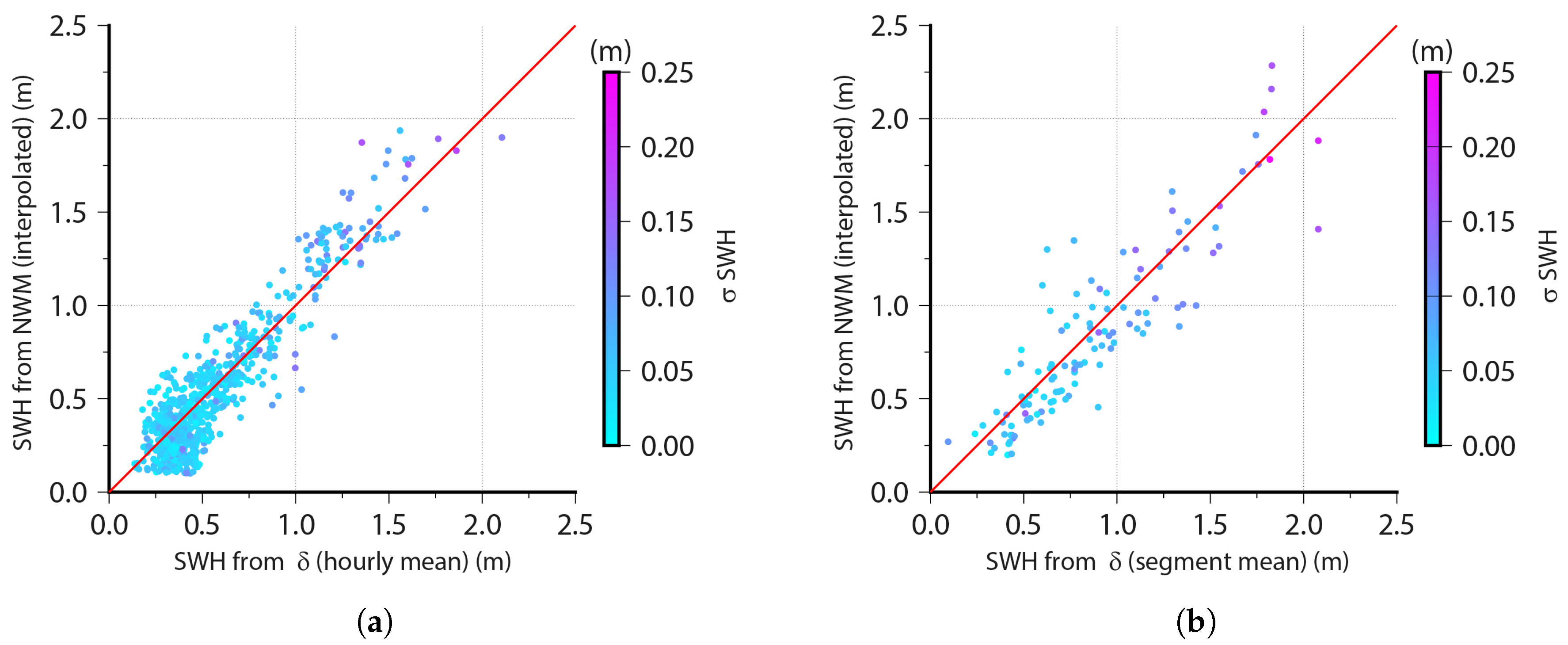
In Figure 5, reference SWH data for both the static experiment (Figure 5a), as well as the kinematic experiment (Figure 5b) are plotted against the damping coefficient derived from SNR analysis. In both cases, the SWH can be assumed to be a linear function of the damping coefficients $\delta$. Hence, a first degree polynomial was fitted to both datasets. Both the buoy data and the estimated $\delta$ values are stochastic variables and have to be treated as such in the adjustment. This was done using a robust total least squat adjustment. Initially, the stochastic model was derived from the estimated standard deviations of the damping coefficients and, due to the lack of accuracy information, an assumed uniform standard deviation of $0.05$ $\mathrm{m}$ for the SWH values. After each solution convergence, the observation weights were adjusted due to the normalized residuals of the observations. This procedure was repeated until a termination criterion was reached. The resulting linear functions are plotted as red lines in Figure 5a,b. The shading of the data relates to the final weights from the robust adjustment.

As expected, the geodetic antenna’s damping was higher for the same SWH values. Hence, this antenna is less affected by multipath effects. The estimated parameters and the standard deviation of unit weight ($s_0$) are shown in

Table 2. Standard deviation of unit weight and estimated parameters of the linear models.

Parameter	Static Antenna m	Moving Antenna m
$s_0$	0.126	0.085
$a_0$	−1.161	−0.157
$a_1$	5.300	3.104

. The $s_0$ of the static experiment was slightly larger than that of the kinematic experiment. This might be a result of the SWH conditions near the coast and the therefore necessary correction term. Nevertheless, since the standard deviations lied in the range of the resolution of the reference in situ SWH observations, the method worked well in both cases.

5. Validation

The linear functions calculated in the previous section describe the SWH as linear functions of the damping coefficients $\delta$ individually for the antenna types and can now be used to calculate SWH from $\delta$. For real applications, it can be assumed that the SWH in a particular area is constant in space and over longer time spans since the SWH is an average measure of roughness and, commonly, changes slowly over time. Therefore, the individually-derived $\delta$ values can be averaged within a reasonable time span. This should increase the quality of the derived SWH. The calculation of a mean $\delta$ should take into account a correct stochastic model that adopts the standard deviations derived from the non-linear robust least squares adjustment. In this way, negative impacts of outliers and false reflections will be down-weighted, as well. The $\delta$ values from the static antenna were sampled into hourly time slots according to their reference epoch. For the moving antenna scenario, all satellites from a segment were used to produce a mean value because the segments were always shorter than one hour. Finally, the SWH was calculated from these mean damping coefficients.

For an independent validation, SWH data that were not used in the previous modeling section are required. Although many altimeter satellite ground tracks cross the German Bight, altimetry data are not useful for validation of this experiments. Due to the long revisit time, too few observations are available. Because of their distance to the measuring sites, data from other wave buoys could not be used either. Even if high frequency radar systems can be used for wave estimation [23], the system that is observing the German Bight [24] was only used for surface current calculation during both experiments. Due to the lack of other suitable data sources, the validation was done in comparison with NWM data. It should be emphasized that the wave model is independent of the buoy measurements used in the previous section because no in situ data were assimilated into the model. Therefore, these data can be used to validate the results obtained from the ship’s measurement without any concern. In the case of the static experiment, differences of SWM estimates from the NWM were used to correct the buoy data. A systematic bias that would have been canceled out by this procedure would still be in the validation data. Hence, the datasets are not completely independent, which may result in an underestimation of uncertainty.

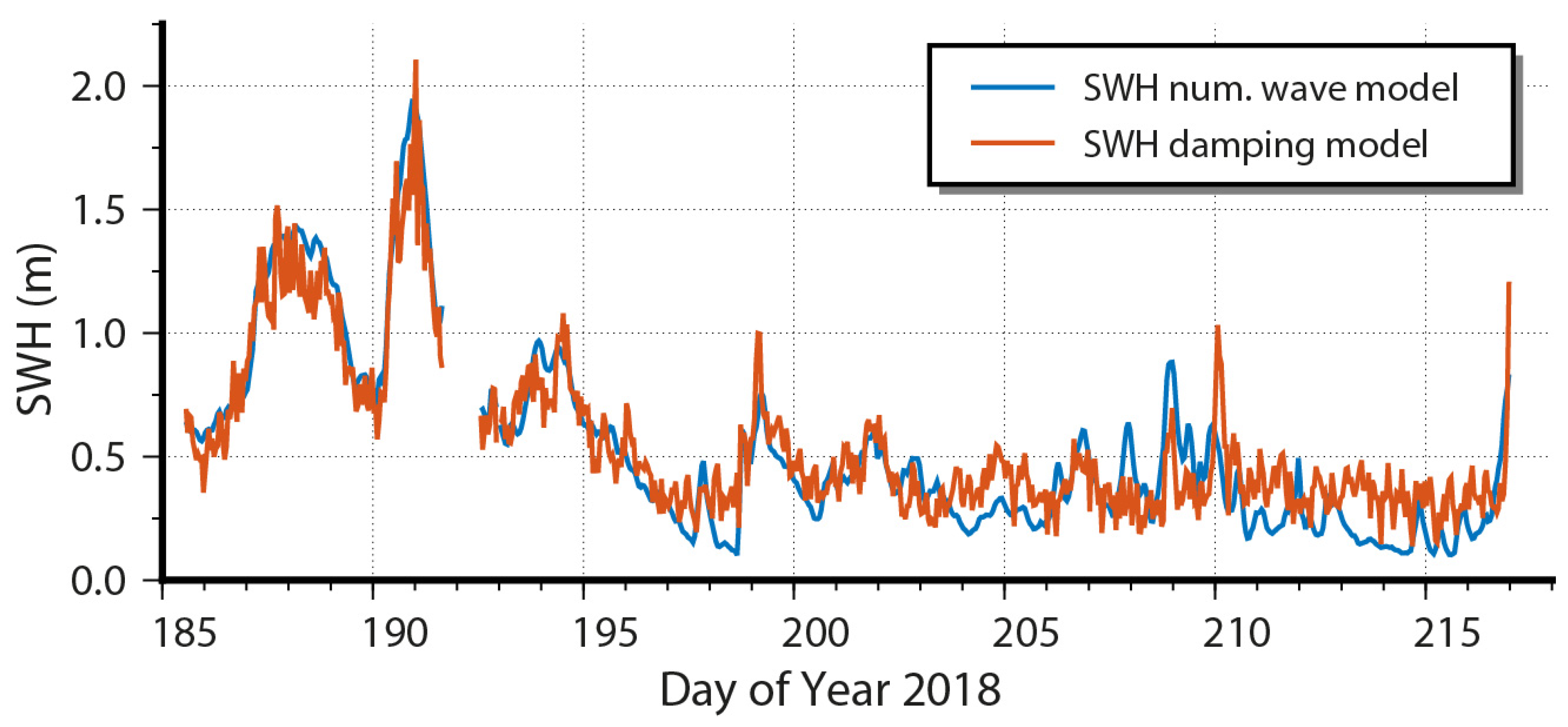
Reference values were interpolated from the NWM results for each hourly slot and ship segment. In total, 733 time slots of the static antenna could be compared. The time series of the reference and of the empirical calculated SWH for the static antenna are shown in Figure 6. The reference series was less noisy, and both series matched well. On average, the differences between SWH from wave model and SWH from the empirical model was $-0.022$ $\mathrm{m}$. The RMS was $0.146$ $\mathrm{m}$. Seventeen percent of all time slots showed differences above $0.20$ $\mathrm{m}$. In Figure 7a, both series are plotted against each other. The correlation coefficient was 0.92, and both high SWH and low SWH values matched well. The average $\sigma$ of the estimates SWH was $0.048$ $\mathrm{m}$. The $\sigma$ increased for higher SWH values, and a maximum of $0.253$ $\mathrm{m}$ was found.

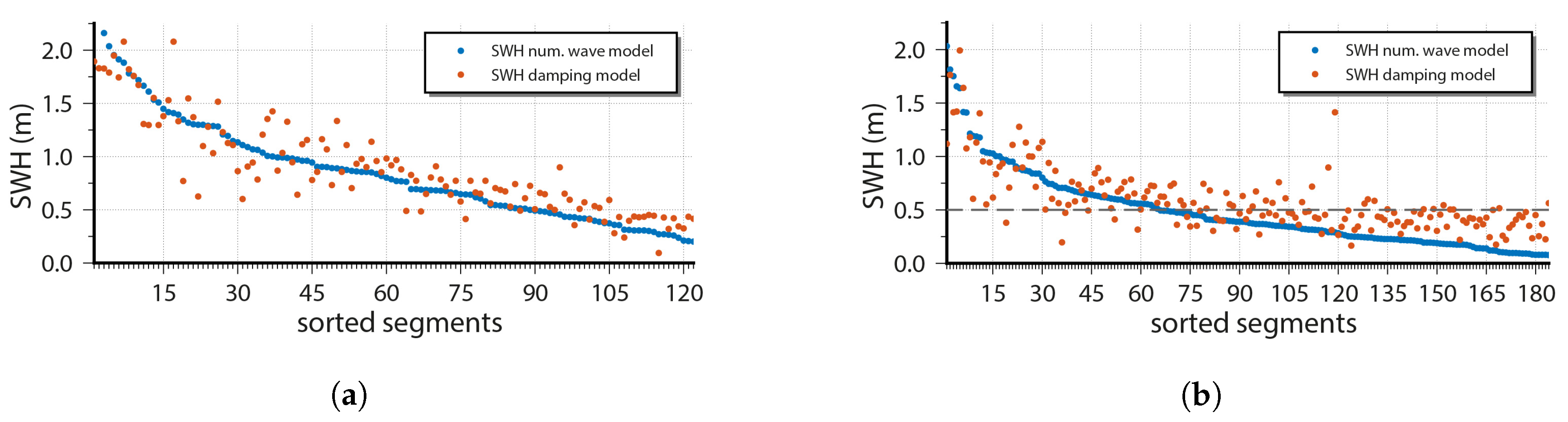
In the case of the data resulting from the ship-based experiment, the validation was split into two parts. First, the deep water segments and second the shallow water segments were compared with the reference values. In Figure 7b, the results from the 122 deep water segments are plotted against the reference values. The mean difference was $-0.030$ $\mathrm{m}$, hence similar to that of the static antenna, but the RMS increased to $0.210$ $\mathrm{m}$. On average, the $\sigma$ of the estimated SWH values was $0.083$ $\mathrm{m}$ and therefore double the size of the value found for the static antenna. Again, the $\sigma$ increased for higher SWH, reaching a maximum $\sigma$ of $0.438$ $\mathrm{m}$. The correlation coefficient between both datasets was 0.90. In Figure 8, the results of both water depth classes, sorted according to the reference SWH, are shown. In the case of the segments with a water depth of more than 25 $\mathrm{m}$ (see Figure 8a), 29% differed more than $0.20$ $\mathrm{m}$ from the reference. More than 50% from these were measured when the SWH was above $1.0$ $\mathrm{m}$. For the 184 segments where the water depth was less than 25 $\mathrm{m}$, the mean difference was significantly larger, reaching $-0.108$ $\mathrm{m}$ (see Figure 8b). Forty two percent of all segments analyzed showed differences of $0.20$ $\mathrm{m}$ and more. For SWH below $0.5$ $\mathrm{m}$, the empirical model results tended to be significantly higher than the reference values.

It can be stated that a significant difference between the validation results of the two water depth classes was found. The reason for the worse performance in shallow water could be searched for by either the reference values or by the results from the empirical model. It cannot completely be ruled out that the reference value from the NWM was only vague estimations in the shallow regions crossed by the ship. In this region, no in situ measurements were available for model verification. Nevertheless, it is unlikely that the discrepancies were caused by the reference values. This is because of the good validation results for the static antenna and because of a comparison done with in situ data in shallow water where no systematic effects were found (see Section 3.3.2). It is therefore more likely that the empirical results were responsible for the systematic differences. These results depend on a precise and accurate estimation of the damping coefficient $\delta$. The estimation requires reliable SNR observations and information about the reflector height $h_{ref,t_i}$. Erroneous observations would result in incorrectly-solved $\delta$ values or may be unsolvable. Such outliers would be down weighted in the average process and would only cause higher noise, but no offset. Because of this, it is most likely that the differences were caused by a systematic effect during the $h_{ref,t_i}$ calculation. The hydrodynamic squat effect can cause such a systematic change of $h_{ref,t_i}$ and therefore a false oscillation frequency in Equation (1). In shallow water, the depth dependence cannot be neglected, and the squat computation becomes more complicated. Better knowledge of the ship specific squat in shallow regions, as well as of the necessary input parameters will lead to improved validation results.

6. Summary

In this work, a method for estimating the significant wave height (SWH) from GNSS reflectometry using the SNR interference pattern was presented. The method uses the damping coefficient $\delta$ of the oscillating SNR signal, which depends on the sea surface roughness and therefore correlates with the SWH. If the reflector height is known, $\delta$ can be estimated using non-linear least squares adjustment. The coefficients from multiple satellites, gathered during different sea state conditions, can further be used for empirical model calculation. The required data can be taken from other SWH sensors like wave buoys or numerical wave models.

The methodology for static antennas, as well as for antennas installed aboard ships was presented. One month of data gathered from a static antenna and three months of data gathered aboard a ship were processed, and the specific processing steps were explained. SWH observations were taken from wave buoys, and if necessary, an additional correction was calculated from a numerical wave model. The estimated function was subsequently used for the calculation of SWH values valid for specific time spans. Due to the lack of useful independent in situ or remote sensing SWH observations, a validation was done with modeled data. Correlation coefficients of 0.92 for the static antenna and of 0.90/0.79 for the ships antenna in deep/shallow water were found. The mean differences were around $-0.02$ $\mathrm{m}$ for the static antenna and $-0.03$ $\mathrm{m}$ for ship measurements in deep water. In shallow water, where the handling of the hydrodynamic squat effect is quite complex, the mean difference was $-0.11$ $\mathrm{m}$.

It can be concluded that GNSS reflectometry based on the analysis of SNR interference pattern is an easy-to-apply technique, especially if existing stations are used. Applying the proposed method, stations located near the coast or on artificial structures could be used to gather observations of the SWH. The ship experiment showed how such data can be handled, as well. Nearly all ships are equipped with GNSS for navigation purposes, but better antennas/receivers are necessary to obtain reliable results. Additionally, the ship’s hydrostatics and hydrodynamics must be known. If all these requirements are fulfilled, measurements from ships will be a great opportunity to gather more SWH data in the open ocean or in areas where no other techniques are available.

Data Availability Statement

The GNSS data used for the static experiment are available from BfG, but restrictions apply to the availability of these data. This data were used under license for the current study, and are not publicly available. Data are however available from the corresponding author upon reasonable request and with permission of BfG. The GNSS data gathered aboard the ferry are not available for the public. These data are part of an other project and still under investigation.

The weather data used in this study are available from DWD and can be downloaded from the Climate Data Center (DWD—Climate Data Center: https://www.dwd.de/EN/climate_environment/cdc/cdc_node.html) for free.

The tide gauge readings used in this study are available from WSV. Registered users can download these data from their online service PEGELONLINE (WSV—PEGELONLINE: https://www.pegelonline.wsv.de/gast/start) for free.

Data from wave buoys used in this study are available from BSH. Registered users can download the Wave buoy data from the COSYNAdata portal (COSYNA data portal: http://codm.hzg.de/codm/) for free. Upon reasonable request, the numerical wave model results can be obtained from DWD and BSH. Data are however available from the corresponding author with permission of both institutions.