Particle Center Supported Plane for Subsurface Target Classification based on Full Polarimetric Ground Penetrating Radar

Abstract

The subsurface target classification of ground penetrating radar (GPR) is a popular topic in the field of geophysics. Among the existing classification methods, geometrical features and polarimetric attributes of targets are primarily used. As polarimetric attributes contain more information of targets, polarimetric decomposition methods, such as H-Alpha decomposition, have been developed for target classification of GPR in recent years. However, the classification template used in H-Alpha classification is preset depending on the experience of synthetic aperture radar (SAR); therefore, it may not be suitable for GPR. Moreover, many existing classification methods require excessive human operation, particularly when outliers exist in the sample (the data set containing the features of targets); therefore, they are not efficient or intelligent. We herein propose a new machine learning method based on sample centers, i.e., particle center supported plane (PCSP). The sample center is defined as the point with the smallest sum of distances from all points in the same sample, which is considered as a better representation of the sample without significant effect of the outliers. In this proposed method, particle swarm optimization (PSO) is performed to obtain the sample centers; the new criterion for subsurface target classification is achieved. We applied this algorithm to full polarimetric GPR data measured in the laboratory and outdoors. The results indicate that, comparing with support vector machine (SVM) and classical H-Alpha classification, this new method is more efficient and the accuracy is relatively high.

1. Introduction

Ground penetrating radar (GPR) is a type of electromagnetic technique for the detection of subsurface targets. It has been applied widely to various fields such as engineering, archaeology, hydrology, and land mine identification. As underground object detection is always involved in these fields, the subsurface target classification of the GPR becomes a popular topic in the geophysical field. It is aimed to classify different types of targets based on their attributes. Among the existing methods, geometrical features and polarimetric attributes are primarily used in classification. For example, Ikechukwu K. Ukaegbu et al. combined GPR and a gamma ray detector to estimate the nonintrusive depth of buried radioactive wastes [1]; Wentao Li et al. applied a randomized Hough transform to achieve the automatic recognition of tree roots [2]; Byeongjin Park et al. used instantaneous phase analysis of GPR data to perform underground object classification [3]; Xuan Feng et al. applied migration for the detection of underground objects [4,5,6]. However, traditional GPR measurements can only yield a small part of information for underground objects. As the full polarimetric data contains much more information of targets [7], full polarimetric GPR has been developed to detect underground objects in recent years [8,9]. Polarimetric decomposition [10,11] is a method for obtaining polarimetric attributes from full polarimetric data, in which H-Alpha decomposition [5] and Freeman decomposition [12,13] have been applied to GPR.

H-Alpha decomposition is a method based on the Kennaugh matrix, which was proposed by Cloude and Pottier in 1997 [14]. This method has been applied widely to synthetic aperture radar (SAR), as well as to target classification in GPR [5] in recent years. It uses entropy H and angle Alpha to perform the classification. The entropy H is a measure of randomness of scattering mechanisms, and the angle Alpha characterizes the scattering mechanism [15]. This classification method depends on the classification template called the H-Alpha plane [5] which contains nine zones, and the physical scattering characteristic associated with each zone provides information for identification. This distinctive advantage, unfortunately, is offset by preset zone boundaries in the H-Alpha plane [15]. The determination of classification boundaries depends on the experience of SAR. While some differences in measurement exist between GPR and SAR, such as the medium and distance of propagation for electromagnetic waves, observation methods, and noise characteristics, the template used in SAR may not be suitable for GPR. In this study, we removed the classical H-Alpha template and studied the characteristics of H and Alpha data; subsequently, we propose a new machine learning method to obtain the new classification criterion.

Particle swarm optimization (PSO) is a new evolutionary algorithm proposed by J. Kennedy and R. Eberhart in 1995 [16]. This algorithm, which is similar to simulated annealing (SA), starts with a random solution and applies iterations to obtain the optimal solution. Unlike other methods, this method uses particles to represent the random solution. In each iteration, every particle will renew its position based on the optimal position that it has bypassed (local optimal solution) and the optimal position all the particles have bypassed (global optimal solution) [17,18]. It is in fact a method to solve the extreme value of an objective function; therefore, we can change the objective function called the fitness function to solve many different problems. The advantages of this algorithm is fast convergence, high-quality solutions, and fewer parameters required for calculation. In recent years, PSO has been applied to full waveform inversion [19,20], magnetotelluric sounding data inversion [21], and unsupervised clustering analysis [22,23,24,25].

Machine learning has been applied widely in many types of disciplines. It primarily focuses on designing algorithms that can obtain laws from a number of samples which are data sets containing the features of targets, and the laws can be used to predict the characteristics of unknown data. In recent years, many machine learning methods have been applied in the GPR field. For example, Xavier Núñez-Nieto et al. applied logistic regression and neural network (NN) techniques to automated landmine and UXO detection [26]; Tao Liu et al. used neural networks to inverse GPR data [27]; Haoqiu Zhou et al. combined full polarimetric GPR and support vector machine (SVM) data for subsurface target classification [28]; Minghe Zhang et al. used freeman decomposition and random forest (RF) to perform underground object detection [29].

In this article, we define the sample center as the point with the smallest sum of distances from all points in the same sample, the sample center is considered a better representation of the sample without significant effects of the outliers. Subsequently, particle center supported plane (PCSP) is proposed to perform the classification.

This article is organized as follows. Section 2 introduces the theory of H-Alpha decomposition, and details the proposed the technique, i.e., particle center supported plane (PCSP). In Section 3, the PCSP is applied to full polarimetric GPR data of four types of targets measured in the laboratory. Section 4 verifies the feasibility of PCSP with real full polarimetric GPR data of underground pipes measured outdoors. In Section 5, an additional experiment is performed for three pipes of different depths, diameters, and materials; subsequently, classical H-Alpha classification and support vector machine (SVM) analysis are performed to compare with the PCSP method.

2. Theory

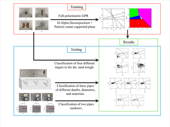
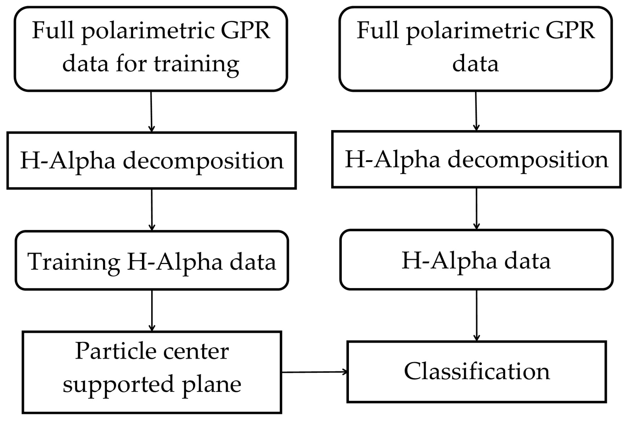
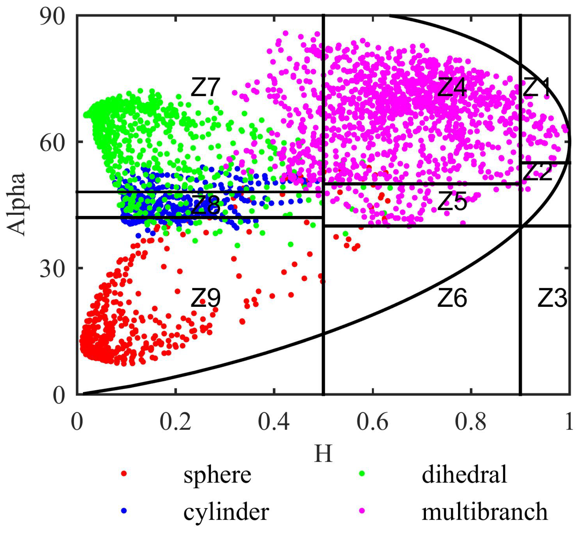
2.1. H-Alpha Decomposition

In full polarimetric GPR, the Sinclair matrix [S] is applied to describe the nature of target scattering. The [S] matrix [13] can be represented as follows:

$$\left[S\right]=\left[\begin{array}{cc}{S}_{HH}& S_{HV}\\ S_{VH}& S_{VV}\end{array}\right]$$

(1)

where S_XY represents the GPR data that is collected with an X type polarimetric receiving antenna and Y type polarimetric transmitting antenna, H represents horizontal polarimetric antenna, V represents vertical polarimetric antenna. According to the reciprocity theorem, S_HV is equal to S_VH.

The scattering vector k_s is defined as follows [4]:

$$k_s=\frac{1}{\sqrt{2}}{\left[\begin{array}{ccc}{S}_{HH}+S_{VV}& S_{HH}-S_{VV}& 2S_{HV}\end{array}\right]}^T$$

(2)

Coherency matrix [T] and its parameterization [4] is shown as (3), where λ₁, λ₂, λ₃, represent eigenvalues, and [U₃] is composed with eigenvectors [4], [U₃] is shown as (4):

$$\left[T\right]=k_s·k_s^{T*}=\left[U_3\right]\left[\begin{array}{ccc}{\lambda }_1& 0& 0\\ 0& {\lambda }_2& 0\\ 0& 0& {\lambda }_3\end{array}\right]{\left[U_3\right]}^{-1}$$

(3)

$$\left[U_3\right]={\left[\begin{array}{ccc}{e}_1& e_2& e_3\end{array}\right]}^T=\left[\begin{array}{ccc}\cos {\alpha }_1& \cos {\alpha }_2& \cos {\alpha }_3\\ \sin {\alpha }_1\cos {\beta }_1{e}^{j{\delta }_1}& \sin {\alpha }_2\cos {\beta }_2{e}^{j{\delta }_2}& \sin {\alpha }_3\cos {\beta }_3{e}^{j{\delta }_3}\\ \sin {\alpha }_1\cos {\beta }_1{e}^{j{\gamma }_1}& \sin {\alpha }_2\cos {\beta }_2{e}^{j{\gamma }_2}& \sin {\alpha }_3\cos {\beta }_3{e}^{j{\gamma }_3}\end{array}\right]$$

(4)

where e₁ e₂ e₃ are the eigenvectors. The parameterization of a 3 × 3 unitary [U₃] matrix in terms of column vectors with different parameters α, β, δ and γ, which are the parameters of the dominant scattering mechanism, is made so as to enable a probabilistic interpretation of the scattering process.

Finally, the mean scattering angle α and entropy H [4] can be calculated as follows:

$$\overline{\alpha }={\displaystyle \sum _{i=1}^3{p}_i{\alpha }_i},H={\displaystyle \sum _{i=1}^3-p_i{\log }_3{p}_i}$$

(5)

where p₁, p₂, p₃ are the false probabilities [4] calculated as follows:

$$\begin{array}{cc}{p}_{i(i=1,2,3)}=\frac{{\lambda }_i}{{\displaystyle {\sum }_{k=1}^3{\lambda }_k}},& {\displaystyle \sum _{k=1}^3{p}_k=1}\end{array}$$

(6)

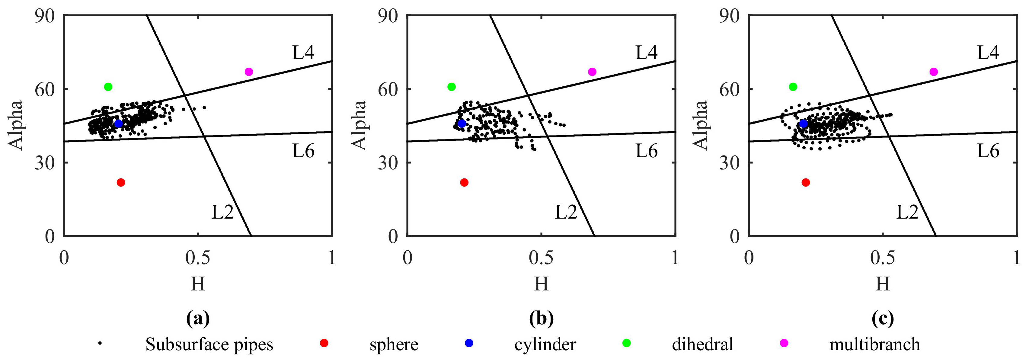
Herein, H and α are the parameters used to perform the classification.

2.2. Particle Center Supported Plane

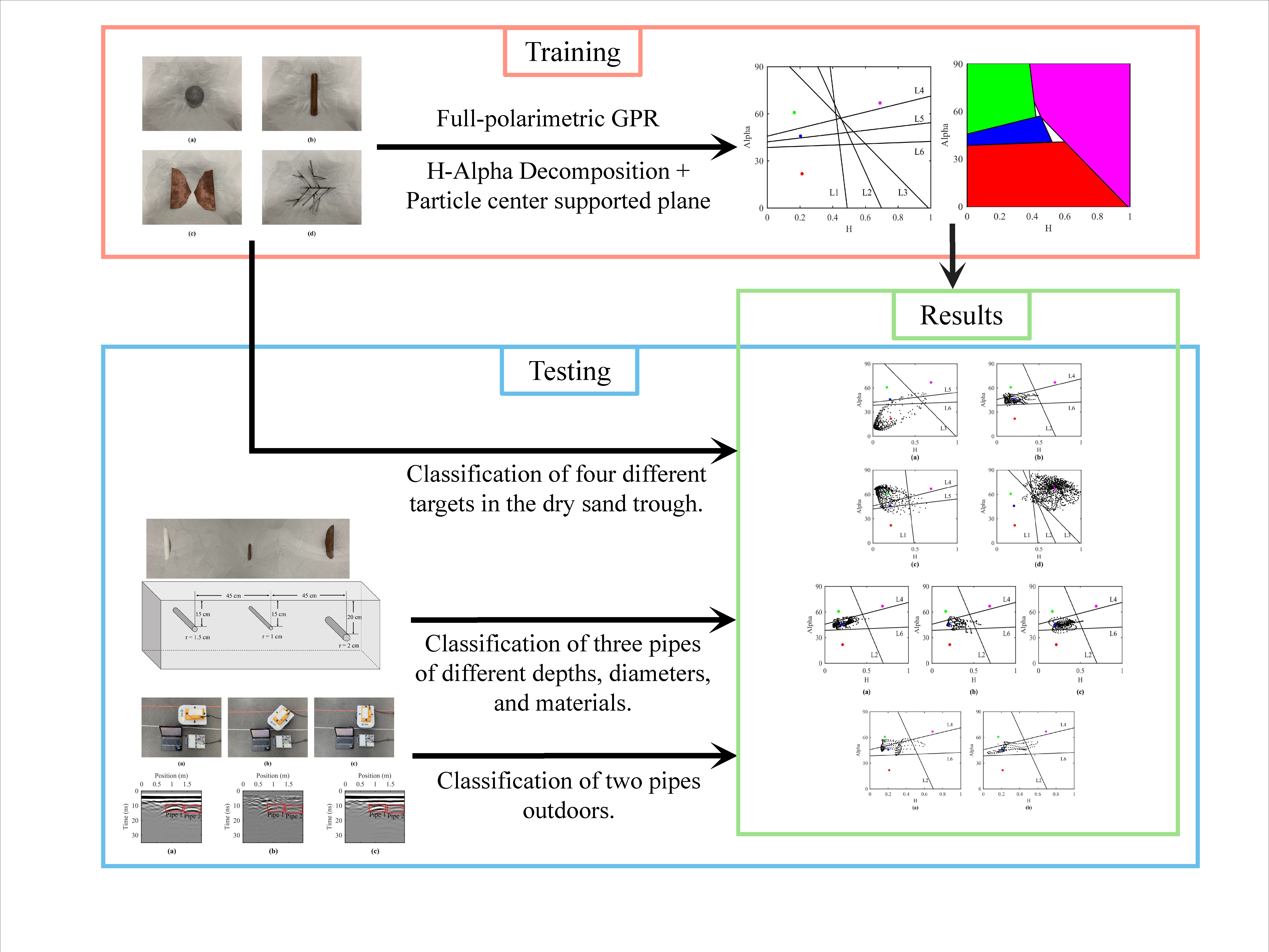
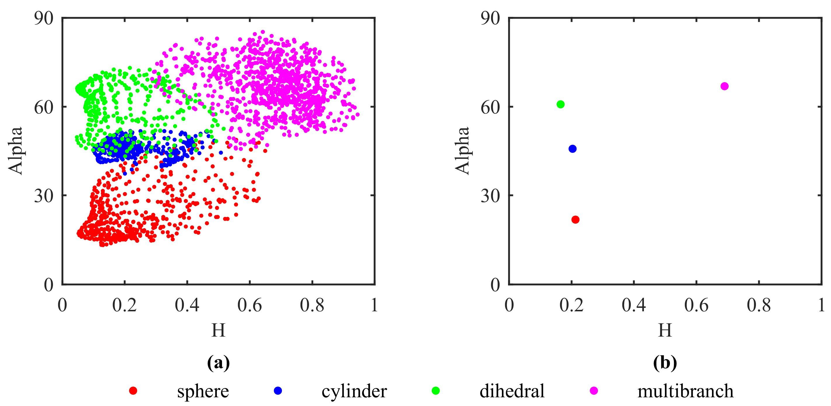
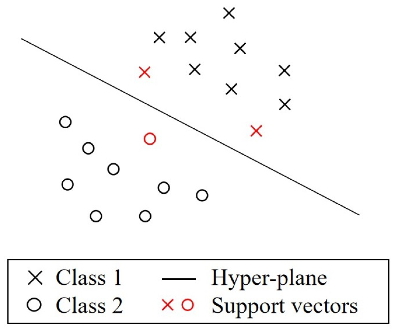
We define the sample center as the point with the smallest sum of distances from all points in the same sample. Typically, some outliers will be present in the sample. These outliers will affect the training result of the classification significantly (Figure 1a), but the effect on the sample center is small. For example, in the quadrilateral ABCD of Figure 1b, the diagonal intersection O is the point with the smallest sum of distances from four points A, B, C, D; therefore, point O is the sample center of points A, B, C, D. However, wherever the outlier C is at the extension line of AC, the sample center O will never change. Therefore, the sample center is considered a better representation of the sample without the significant effects of the outliers.

In this research, we propose a new machine learning method based on sample centers, i.e., particle center supported plane (PCSP), to perform the classification. The sample centers are obtained by particle swarm optimization (PSO). For PSO, particles are used to represent the random solutions of the optimization problem. The coordinate and velocity of mth particle at kth iteration can be represented as follows [22]:

$$x_m^k=\left(x_{mH}^k,x_{m\alpha }^k\right),m=1,2,\dots ,M$$

(7)

$$v_m^k=\left(v_{mH}^k,v_{m\alpha }^k\right),m=1,2,\dots ,M$$

(8)

where M represents the number of particles, and k is the time of iteration, $x_{mH}^k$ and $x_{m\alpha }^k$ correspond to H and α coordinates, respectively. The initial position $x_m^0$ and initial velocity $v_m^0$ are random.

In this problem, the sample contains H and α, therefore, the training sample can be represented as follows:

$$z_{tni}=\left[H_{tni},{\alpha }_{tni}\right],n=1,2,\dots ,N_i,i=1,2,\dots ,P$$

(9)

where z_tni represents the nth training sample point in ith type; t represents “training”; N_i is the number of sample points in z_tni; P represents the number of types.

We want the sum of the distances between the particles and all the points in the same sample to be minimum. Therefore, the objective function (fitness function) is defined as follows:

$$Fit(x_m^k)={\displaystyle \sum _{n=1}^N\sqrt{{\left(x_{mH}^k-H_{tni}\right)}^2+{\left(x_{m\alpha }^k-{\alpha }_{tni}\right)}^2}},m=1,2,\dots ,M$$

(10)

From the first iteration to the kth iteration, the minimum value of the fitness function for mth particle is known as the local optimal solution of mth particle at kth iteration, i.e., $B_m^k$, m = 1,2,…,M; the minimum value of the fitness function for all the particles is known as the global optimal solution at kth iteration, i.e., $B_g^k$ [22].

For all particles, we use the formulas below to renew their positions and velocities [22]:

$$v_m^{k+1}=\omega v_m^k+c_1{r}_1\left(B_m^k-x_m^k\right)+c_2{r}_2\left(B_g^k-x_m^k\right)$$

(11)

$$x_m^{k+1}=x_m^k+v_m^{k+1}$$

(12)

where k represents the time of iteration; ω is the inertia weight; r₁, r₂ are the random numbers between 0 to 1; c₁, c₂ are the learning factors. In fact, for the right part of Equation (11), the first item represents the impact of the current position, the second item represents the impact of the current optimal position of this one particle, and the third item represents the influence of current optimal position of all particles. When the fitness function becomes minimum, the particles are at the center of the sample, the coordinate of sample center is B_g, subsequently, we can obtain the sample centers of all types of samples:

$$Fit\left(B_g\right)=\min Fit\left(x\right)$$

(13)

$$B_g=\left(B_{g1},B_{g2},\dots ,B_{gP}\right)$$

(14)

where P represents the number of classes.

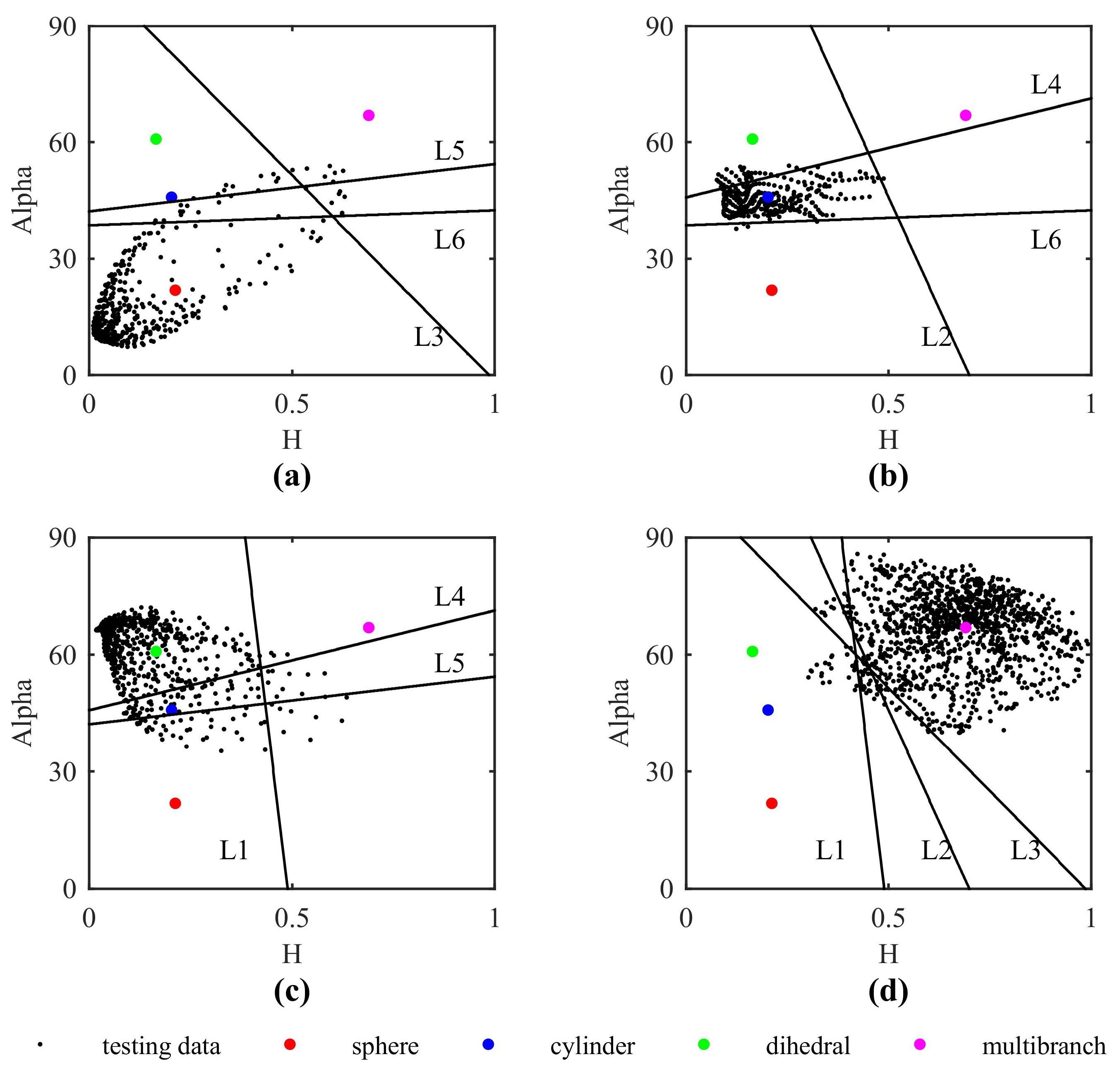
After the sample centers of different samples are achieved from PSO, a classification law can be constructed based on these sample centers. Figure 1a indicates that the outliers can affect the slope of the classification boundary significantly. In this method, straight lines are used as the classification boundary, and the slope of every line is determined by the sample centers. Subsequently, the intercepts are calculated by the classification accuracy for training samples.

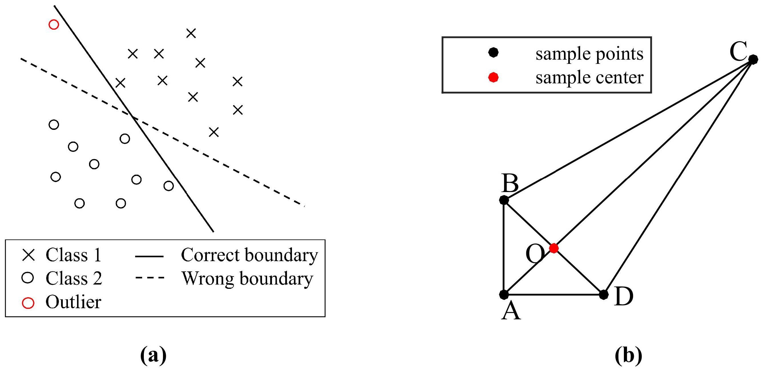
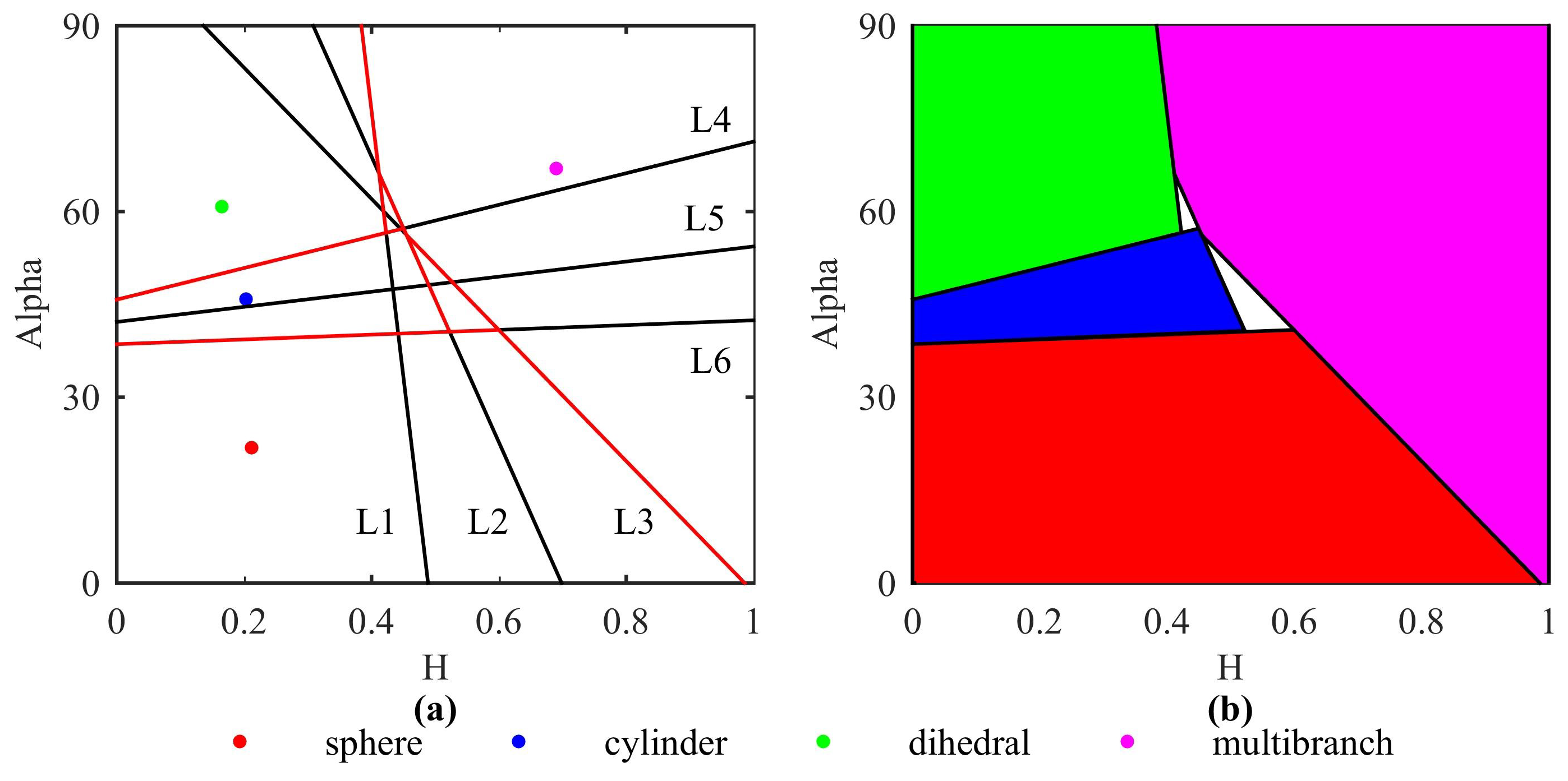
For all the training samples {z_tn1, z_tn2,…,z_tnP} and their sample centers {B_g1, B_g2,…, B_gP}, where P is the number of classes, we use {z_tni, z_tnj} and their sample centers {B_gi, B_gj} as examples. In Figure 2a, red points and purple points belong to the ith type, green points and blue points belong to the jth type. A critical point Q_ij between two sample centers is calculated based on the classification accuracy of the boundary Line_ij. The Line_ij is through the critical point Q_ij and is perpendicular to the connection line of B_gi and B_gj; the equation of Line_ij is as follows:

$${\mathrm{Line}}_{ij}:\left(B_{gj}-B_{gi}\right)\cdot \left(z-Q_{ij}\right)=0$$

(15)

where z = (H, α) is the point on the flat.

The points that are on the same side of Line_ij with B_gi are considered to belong to the ith type. The accuracy of Line_ij for classifying ith type and jth type are as follows, respectively:

$$Accurac{y}_i=\frac{N_i\left(\left(z_{tni}-Q_{ij}\right)·\left(B_{gi}-Q_{ij}\right)>0\right)}{N_i}$$

(16)

$$Accurac{y}_j=\frac{N_j\left(\left(z_{tnj}-Q_{ij}\right)·\left(B_{gj}-Q_{ij}\right)>0\right)}{N_j}$$

(17)

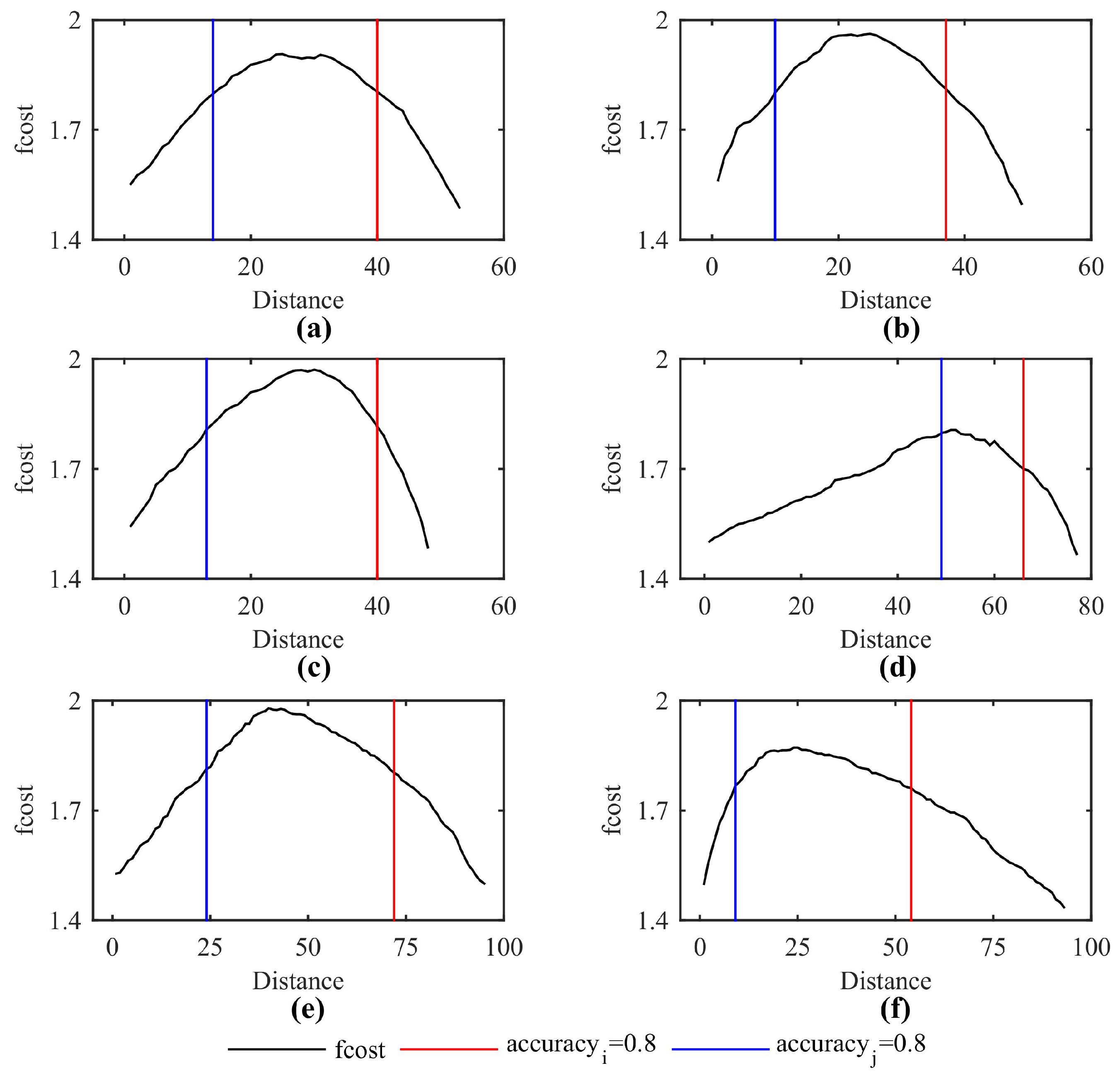
where N_i ((z_tni − Q_ij)∙(B_gi − Q_ij) > 0) represents the number of points in the ith sample which is on the same side of Line_ij with B_gi. Subsequently, the points in the ith sample that are far away from the sample center B_gi are considered as outliers; therefore, Accuracy_i and Accuracy_j do not have to be 1. We chose Accuracy_i,j = 0.8 as the threshold. The objective function is defined as follows:

$$fcost=Accurac{y}_i+Accurac{y}_j$$

(18)

$$Accurac{y}_{i,j}\ge 0.8$$

(19)

Subsequently, the optimal Q_ij as well as the particle center supported plane Line_ij can be determined by solving the maximum value of (18) under the condition of (19).

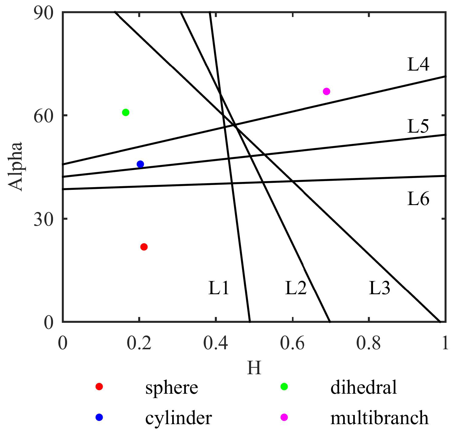
By repeating the above steps, all the boundary lines between every two samples of {z_tn1, z_tn2,…,z_tnP} can be determined. Subsequently, classification can be performed for the new data z_cn where c represents “classified”. The discriminant function for the ith type with the other jth type is as follows:

$$f_{ij}\left(B_{gj},z_{cn}\right)=sign\left\{\left(B_{gi}-Q_{ij}\right)·\left(z_{cn}-Q_{ij}\right)\right\}$$

(20)

where j = 1,2,…,P, j ≠ i. The complete discriminant function of the ith type is:

$$F_i(z_{cn})=-1+\frac{1}{P-1}{\displaystyle \sum _{j=1,j\ne i}^P{f}_{ij}\left(B_{gj},z_{cn}\right)}$$

(21)

If F_i (z_cn) = 0, z_cn belongs to the ith type. As Figure 2b shows, if the new sample point is on the same side of the red line with B_g1, it belongs to the type of B_g1.

2.3. Data Processing Flow Chart

The Data processing flow chart of the proposed method is in Figure 3. Firstly, the H-Alpha decomposition is performed to obtain the H and α data for training; subsequently the particle center supported plane (PCSP) is performed to obtain the classification boundaries; finally, the new H-Alpha data is applied to the PCSP to obtain the classification result.

3. Data Analysis of Typical Targets in the Laboratory and Outdoors

In this section, full polarimetric GPR data measured in the laboratory was applied to the proposed method to obtain the classification boundaries and verify its feasibility.

3.1. Full polarimetric GPR Measurement

The full polarimetric measurements of four types of targets (Figure 4) were performed in the laboratory. The survey lines were right on the targets, the number of measurement points was 101, the measurement point interval was 1 cm, the frequency ranges between 800 MHz and 4000 MHz, and the number of sampling points was 1024. The four typical targets are as follows: metallic sphere, representing Bragg surface scattering; metallic cylinder, representing linear body scattering; metallic dihedral, representing double-bounce scattering; and metallic multibranch, representing multiple scattering. The diameter of the sphere was 15 cm. The length of the cylinder was 31.5 cm, the diameter was 5 cm. The dihedral was made of two plates at a 90° angle whose length and width were 35 cm and 20 cm, respectively. The length of the multibranch scatterer was approximately 40 cm. The four targets were immersed in a dry sand trough whose length, width and depth were 2.53 m, 2.53 m, and 0.85 m, respectively; the wave velocity of the sand was approximately 0.2 m/ns. The buried depths for the top of the sphere and cylinder were 8 cm; the buried depth for the intersection of two plates was 20 cm; the buried depth for the trunk of the multibranch scatterer was 10 cm.

In the measurement, a vector network analyzer and a Cartesian coordinate robot (Figure 5) with different antenna combinations (Figure 6) were used for data collection, the interval between feeding points of transmitting and receiving antennas was 8 cm for all three polarimetric modes with the same axis direction. The data of the sphere, cylinder, dihedral, and multibranch are shown in Figure 7, Figure 8, Figure 9 and Figure 10, respectively.

3.2. H-Alpha Decomposition for GPR Data

After the collection for the full polarimetric GPR data of four types of targets, H-Alpha decomposition is applied to obtain the H and α data. Subsequently, the data of four targets are divided into two equal parts: the training data and the testing data. Figure 11a shows the spatial distribution of the training H and α data of four types of targets.

3.3. Particle Center Supported Plane

Subsequently, PSO is performed for the H and α data to obtain the sample centers of the four types of targets. Twenty particles are used in the calculation (M = 20), and we chose w = 0.5, c₁ = 1.5, c₂ = 2.5; when the relative error between the kth iteration and (k+1)th iteration is under 0.01, the calculation will stop. Figure 11b shows the sample centers of the training data.

In Figure 12, the objective functions of every two sample centers are presented, the right part of the blue line is the range where Accuracy_i > 0.8, and the left part of the red line is the range where Accuracy_j > 0.8. Therefore, we must obtain the maximum value of fcost (shown in (18)) between the blue line and red line. The “Distance” coordinate corresponding to the maximum value of fcost indicates the best position of Q_ij at the connection line of B_gi and B_gj. The obtained boundaries are shown in Figure 13 and the classification types of six boundaries are shown in

Table 1. The types of six boundaries.

Boundary	L1	L2	L3	L4	L5	L6
Type	multibranch	multibranch	multibranch	dihedral	dihedral	cylinder
	dihedral	cylinder	sphere	cylinder	sphere	sphere

.

L1 is the line between the multibranch and dihedral; L2 is the line between the multibranch and cylinder; L3 is the line between the multibranch and sphere; L4 is the line between the dihedral and cylinder; L5 is the line between the dihedral and sphere; L6 is the line between the cylinder and sphere. We used these six lines to classify the testing data; the classification results and accuracy are shown in Figure 14 and

Table 2. Accuracy of particle center supported plane.

Target	Accuracy (%)
Sphere	91.63
Cylinder	86.76
Dihedral	80.89
Multibranch	92.74

, respectively.

The Figure 14 and Table 2 indicate that PCSP can classify these four types of targets with good accuracy. All the correct rates are greater than 80%. In fact, not all the lines contributed to the classification. After some analyses, the real plane partition is shown in Figure 15. The red lines in Figure 15a are the lines which contributed to the classification, the real classification plane is as Figure 15b.

4. Identification for Real Data of Subsurface Pipes

According to Yue Yu [30], we can use the single polarimetric GPR to obtain the full polarimetric GPR data. Three time measurements with different measuring angles of antenna directions and survey direction are applied in this method as Figure 16 shows. We assume that the data collected by using this method are M_0°, M_45°, and M_90°, respectively, the real matrix [S] can be represented as (22) [30].

$$S=\left[\begin{array}{cc}{M}_{0^{°}}& M_{{45}^{°}}-\frac{M_{0^{°}}+M_{{90}^{°}}}{2}\\ M_{{45}^{°}}-\frac{M_{0^{°}}+M_{{90}^{°}}}{2}& M_{{90}^{°}}\end{array}\right]$$

(22)

We applied this method to the data collection of subsurface pipes using 500 MHz shielded MALA GPR. The buried depths of two pipes were approximately 0.5 m and 0.55 m; the pipes extend two hundred meters in the north-south direction; the estimated pipe diameters were both approximately 20 cm; the applied GPR system had two horizontal polarimetric antennas whose interval is 18 cm. The number of measurement points was 98; the measurement point distance was 2 cm; the number of sampling points was 600. The applied GPR system and three types of measuring methods are shown in Figure 17. The full-polarimetric data obtained by using (22) are shown in Figure 18; the red rectangles indicate the positions of two subsurface pipes. The classification result of PCSP is shown in Figure 19. The accuracy is shown in

Table 3. Classification probability of subsurface pipes.

Target	Probability of Sphere (%)	Probability of Cylinder (%)	Probability of Dihedral (%)	Probability of Multibranch (%)
Pipe 1	1.26	68.91	28.57	4.62
Pipe 2	0.51	72.31	7.69	6.15

.

Figure 19 shows that majority of the data points of three pipes focused on the blue zone. Table 3 shows that for the two pipes, the probabilities that they belonged to the type of cylinder were far higher than the other three types, the probabilities were 68.91% and 72.31%, respectively.

5. Discussion

5.1. Identification for Three Pipes of Different Depths, Diameters and Materials.

To verify the feasibility of the proposed method. An additional experiment was performed. In this experiment, three pipes (Figure 20) of different depths, diameters, and materials were buried in the dry sand trough. The measurement environment and instruments were the same with that of Section 3.1. The parameters and buried states of three pipes are in

Table 4. The parameters of three pipes.

Target	Depth (cm)	Diameter (cm)	Material
Pipe 1	15	3	PVC
Pipe 2	15	2	Metallic
Pipe 3	20	4	Metallic

and Figure 21, respectively. The distance between the three pipes was 45 cm. The survey lines were right on the targets, the number of measurement points was 89, the measurement point interval was 2 cm, the frequency ranged between 800 MHz and 4000 MHz, and the number of sampling points was 1024.

The measurement data are shown in Figure 22. Subsequently, we perform the PCSP to identify these three pipes. The identification results and accuracy are shown in Figure 23 and

Table 5. Identification accuracy of three pipes.

Target	Probability of Sphere (%)	Probability of Cylinder (%)	Probability of Dihedral (%)	Probability of Multibranch (%)
Pipe 1	0.00	88.69	10.71	0.30
Pipe 2	7.22	80.56	6.67	2.78
Pipe 3	6.54	88.24	2.61	1.31

, respectively.

The Figure 23 and Table 5 indicate that for the three pipes of different depths, diameters, and materials, most of the data points focused on the blue zone; the probabilities that they belonged to the type of cylinder are far higher than that of other three types, the probabilities were 88.69%, 80.56%, and 88.24%, respectively. The results prove that, for the pipes of different depths, diameters, and materials, the PCSP method can identify them with good accuracy, therefore the proposed method is appropriate.

5.2. Comparison with Classical H-Alpha Classification and Support Vector Machine (SVM)

In this section, classical H-Alpha classification and support vector machine (SVM) were performed to compare with the PCSP method. Classical H-Alpha classification is based on the classical template of SAR with nine zones (Figure 24), and the physical scattering characteristic associated with each zone provides information for classification [14].

Support Vector Machine (SVM) is a new method of pattern recognition which was put forward by Corinna Cortes and Vapnik in 1995 [31]. It has been applied to target classification for GPR [27]. This method uses a hyper-plane to classify two different samples. The support vector is defined as the points in the two samples which are nearest to the hyper-plane, they are the most significant points to determine the hyper-plane and hard to be classified. The key idea is to minimize the spaces between support vectors and the plane to search for the optimal hyper-plane (Figure 25).

The classical H-Alpha classification is an unsupervised method which does not need a training process; SVM is a supervised method which needs a training process. Therefore, the training data used in the SVM was the same as that of PCSP. The same testing data was applied in three methods. The sample points of testing data are projected into the classical H-Alpha classification space as Figure 26 presents.

From Figure 26, we can find that most sample points were in the zones they belong to, but the proportions were not high, particularly for cylinder and multibranch. Subsequently, the proportions of the sample points of the four targets in their zones were calculated; the SVM with linear kernel (L-SVM) was performed. The comparison of accuracy is shown in

Table 6. Comparison of accuracy.

	Methods	L-SVM	H-Alpha	PCSP
Targets
Sphere		90.99	91.87	91.63
Cylinder		81.29	47.35	86.76
Dihedral		77.89	87.70	80.89
Multibranch		92.74	74.53	92.74

; the comparisons of operation time and RAM usage for L-SVM and PCSP are shown in

Table 7. Comparisons of operation time and RAM usage.

Comparison Parameters	L-SVM	PCSP
Operation time (s)	10.067	5.841
RAM usage (MB)	2825	3034

.

Table 6 shows that the accuracy of L-SVM and PCSP were in the acceptable range, and the accuracy of PCSP was slightly higher than that of L-SVM. The correct rates were different with different targets. However, for the H-Alpha method, the accuracy of cylinder classification was under 50%, which means the cylinder can not be identified by using this method.

Table 7 shows that the RAM usage of PCSP is slightly higher than that of L-SVM. However, the operation time of PCSP was obviously less than that of L-SVM. In general, when RAM is sufficient, the accuracy of PCSP is slightly higher than that of L-SVM, and the calculation speed of PCSP is obviously faster than that of L-SVM.

5.3. Limitations of the Proposed Technique

However, the proposed technique for the underground object classification of GPR data are based on the classical parameters (H, α) obtained by H-Alpha decomposition; the type of objects we classified in this study was limited. Follow-up studies are underway to perform the classification for more types of objects using different polarimetric attributes and machine learning methods.

6. Conclusions

In this article, we proposed the particle center supported plane (PCSP) as a classification method based on sample centers to classify the H-Alpha data of ground penetrating radar. To verify the method, the PCSP method was performed to classify both data measured in the laboratory and real data measured on the road outdoors. The results indicate that this method could classify the four types of targets and subsurface pipes with good accuracy. To verify the feasibility of the proposed method, the identification for three pipes of different depths, diameters, and materials were performed, the results indicate that the PCSP method can identify the pipes of different depths, diameters, and materials with good accuracy. To verify the superiority of the proposed method, comparisons between the new method and classical H-Alpha classification, as well as L-SVM, were performed. The comparison of accuracy indicates that the accuracy of L-SVM and PCSP are in the acceptable range, and the accuracy of PCSP is slightly higher than that of L-SVM. However, for the H-Alpha method, the accuracy of cylinder classification was under 50%, which means the cylinder can not be identified by using the H-Alpha method. Moreover, the comparison of operation time and RAM usage indicate that if RAM usage is sufficient, the calculation speed of PCSP is obviously faster than that of L-SVM.

References

1. Ukaegbu, I.K.; Gamage, K.A.A.; Aspinall, M.D. Nonintrusive Depth Estimation of Buried Radioactive Wastes Using Ground Penetrating Radar and a Gamma Ray Detector. Remote Sens. 2019, 11, 141. [Google Scholar] [CrossRef]
2. Li, W.T.; Cui, X.H.; Guo, L.; Chen, J.; Chen, X.H.; Cao, X. Tree Root Automatic Recognition in Ground Penetrating Radar Profiles Based on Randomized Hough Transform. Remote Sens. 2016, 8, 430. [Google Scholar] [CrossRef]
3. Park, B.; Kim, J.; Lee, J.; Kang, M.S.; An, Y.K. Underground Object Classification for Urban Roads Using Instantaneous Phase Analysis of Ground-Penetrating Radar (GPR) Data. Remote Sens. 2018, 10, 1417. [Google Scholar] [CrossRef]
4. Feng, X.; Yu, Y.; Liu, C.; Fehler, M. Subsurface polarimetric migration imaging for full polarimetric ground-penetrating radar. Geophys. J. Int. 2015, 202, 1324–1338. [Google Scholar] [CrossRef]
5. Feng, X.; Yu, Y.; Liu, C. Combination of H-Alpha Decomposition and Migration for Enhancing Subsurface Target Classification of GPR. IEEE Trans. Geosci. Remote Sens. 2015, 53, 4852–4861. [Google Scholar] [CrossRef]
6. Feng, X.; Sato, M. Pre-stack migration applied to GPR for landmine detection. Inverse Prob. 2004, 20, 99–115. [Google Scholar] [CrossRef]
7. Böniger, U.; Tronicke, J. Subsurface Utility Extraction and Characterization: Combining GPR Symmetry and Polarization Attributes. IEEE Trans. Geosci. Remote Sens. 2011, 50, 736–746. [Google Scholar] [CrossRef]
8. Sassen, D.S.; Everett, M.E. 3D polarimetric GPR coherency attributes and full-waveform inversion of transmission data for characterizing fractured rock. Geophysics 2008, 74, J23–J34. [Google Scholar] [CrossRef]
9. Kevin, O. Discrimination of UXO in Soil Using Broadband Polarimetric GPR Backscatter. IEEE Trans. Geosci. Remote Sens. 2001, 39, 356–367. [Google Scholar]
10. Cloude, S.R.; Pottier, E. A review of target decomposition theorems in radar polarimetry. IEEE Trans. Geosci. Remote Sens. 1996, 34, 498–518. [Google Scholar] [CrossRef]
11. Freeman, A.; Durden, S.L. A three-component scattering model for polarimetric SAR Data. IEEE Trans. Geosci. Remote Sens. 1998, 36, 963–973. [Google Scholar] [CrossRef]
12. Feng, X.; Yu, Y.; Lu, Q. Application of freeman decomposition to full polarimetric GPR. In Proceedings of the 2013 IEEE Geoscience and Remote Sensing Symposium (IGARSS), Melbourne, VIC, Australia, 21–26 July 2013; pp. 3534–3537. [Google Scholar]
13. Feng, X.; Liang, W.J.; Liu, C. Application of Freeman decomposition to full polarimetric GPR for improving subsurface target classification. Signal Process. 2017, 132, 284–292. [Google Scholar] [CrossRef]
14. Cloude, S.R.; Pottier, E. An entropy based classification scheme for land applications of polarimetric SAR. IEEE Trans. Geosci. Remote Sens. 1997, 35, 68–78. [Google Scholar] [CrossRef]
15. Lee, J.S.; Grunes, M.R. Unsupervised Classification Using Polarimetric Decomposition and the Complex Wishart Classifier. IEEE Trans. Geosci. Remote Sens. 1999, 37, 2249–2258. [Google Scholar]
16. Kennedy, J.; Eberhart, R. Particle Swarm Optimization. In Proceedings of the ICNN’95—International Conference on Neural Networks, Perth, WA, Australia, 27 November–1 December 1995; pp. 1942–1948. [Google Scholar]
17. Shi, Y.; Eberhart, R. A modified particle swarm optimizer. In Proceedings of the 1998 IEEE World Congress on Computational Intelligence, Anchorage, AK, USA, 4–9 May 1998; pp. 69–73. [Google Scholar]
18. Kennedy, J. The particle swarm: social adaptation of knowledge. In Proceedings of the 1997 IEEE International Conference on Evolutionary Computation (ICEC ’97), Indianapolis, IN, USA, 13–16 April 1997; pp. 303–308. [Google Scholar]
19. Zhu, T.; Li, X.F. PSO-gradient algorithm and its application to seismic waveform inversion for velocity structure in frequency domain. Prog. Geophys. 2013, 28, 0180–0189. [Google Scholar]
20. Zheng, S.; Zhang, A.X. Ground Penetrating Radar Inversion Algorithm Based on Improved Particle Swarm Optimization. J. Electron. Inf. Technol. 2014, 36, 2717–2722. [Google Scholar]
21. Shi, X.M.; Xiao, M. The damped PSO algorithm and its application for magnetotelluric sounding data inversion. Chinese J. Geophys. 2009, 52, 1114–1120. (In Chinese) [Google Scholar]
22. Wang, Y.F. The Particle Swarm Optimization and its Application. Master’s Thesis, Huazhong University of Science and Technology, Wuhan, China, 2008. [Google Scholar]
23. Chouhan, R.; Purohit, A. An approach for document clustering using PSO and K-means algorithm. In Proceedings of the 2nd International Conference on Inventive Systems and Control (ICISC), Coimbatore, India, 19–20 January 2018; pp. 1380–1384. [Google Scholar]
24. Mir, M.; Tadayon Tabrizi, G. Improving data clustering using fuzzy logic and PSO algorithm. In Proceedings of the 20th Iranian Conference on Electrical Engineering (ICEE2012), Tehran, Iran, 15–17 May 2012; pp. 784–788. [Google Scholar]
25. Davodi, M.; Modares, H. Coherency approach by hybrid PSO, K-Means clustering method in power system. In Proceedings of the 2008 IEEE 2nd International Power and Energy Conference, Johor Bahru, Malaysia, 1–3 December 2008; pp. 1203–1207. [Google Scholar]
26. Núñez-Nieto, X.; Solla, M.; Gómez-Pérez, P.; Lorenzo, H. GPR Signal Characterization for Automated Landmine and UXO Detection Based on Machine Learning Techniques. Remote Sens. 2014, 6, 9729–9748. [Google Scholar] [CrossRef]
27. Liu, T.; Su, Y.; Huang, C.L. Inversion of Ground Penetrating Radar Data Based on Neural Networks. Remote Sens. 2018, 10, 730. [Google Scholar] [CrossRef]
28. Zhou, H.Q.; Feng, X. Combination of Support Vector Machine and H-Alpha Decomposition for Subsurface Target Classification of GPR. In Proceedings of the 17th International Conference on Ground Penetrating Radar (GPR), Rapperswil, Switzerland, 18–21 June 2018; pp. 635–638. [Google Scholar]
29. Zhang, M.H.; Feng, X. Full-polarimetric Ground Penetrating Radar Underground Objects Classification Using Random Forest. In Proceedings of the 17th International Conference on Ground Penetrating Radar (GPR), Rapperswil, Switzerland, 18–21 June 2018; pp. 689–693. [Google Scholar]
30. Yu, Y. Development of H-Alpha Feature Decomposition Technology for Full-polarimetric Ground Penetrating Radar. Ph.D. Thesis, Jilin University, Changchun, China, 2016. [Google Scholar]
31. Cortes, C.; Vapnik, V. Support-vector networks. Mach. Learn. 1995, 20, 273–297. [Google Scholar] [CrossRef]
Figure 1. Outlier and sample center. (a) The influence of outlier, where Class 1 and Class 2 represent the samples of two different type of targets. (b) Sample center of four points.
Remotesensing 11 00405 g001
Figure 2. Particle center supported plane. (a) Calculation of a boundary. (b) Discriminant process.
Remotesensing 11 00405 g002
Figure 3. Data processing flow chart.
Remotesensing 11 00405 g003
Figure 4. Four types of targets in the dry sand trough. (a) Metallic sphere. (b) Metallic cylinder. (c) Metallic dihedral. (d) Metallic multibranch.
Remotesensing 11 00405 g004
Figure 5. Full polarimetric ground penetrating radar (GPR) measurement system.
Remotesensing 11 00405 g005
Figure 6. Three types of antenna combinations. (a) HH polarization. (b) HV polarization. (c) VV polarization. H represents horizontal polarimetric antenna, V represents vertical polarimetric antenna.
Remotesensing 11 00405 g006
Figure 7. Full polarimetric data of metallic sphere. (a) HH polarization. (b) HV polarization. (c) VV polarization.
Remotesensing 11 00405 g007
Figure 8. Ful polarimetric data of metallic cylinder. (a) HH polarization. (b) HV polarization. (c) VV polarization.
Remotesensing 11 00405 g008
Figure 9. Full polarimetric data of metallic dihedral. (a) HH polarization. (b) HV polarization. (c) VV polarization.
Remotesensing 11 00405 g009
Figure 10. Full polarimetric data of metallic multibranch. (a) HH polarization. (b) HV polarization. (c) VV polarization.
Remotesensing 11 00405 g010
Figure 11. Particle swarm optimization (PSO) for H-Alpha data. (a) Training H-Alpha data before PSO. (b) Sample centers after PSO iteration.
Remotesensing 11 00405 g011
Figure 12. Fcost and thresholds of six boundaries. (a) Multibranch and dihedral. (b) Multibranch and cylinder. (c) Multibranch and sphere. (d) Dihedral and cylinder. (e) Dihedral and sphere. (f) Cylinder and sphere.
Remotesensing 11 00405 g012
Figure 13. All boundary lines.
Remotesensing 11 00405 g013
Figure 14. Classification result of four types of targets. (a) Sphere. (b) Cylinder. (c) Dihedral. (d) Multibranch.
Remotesensing 11 00405 g014
Figure 15. The real classification plane. (a) Lines that make contribution to the classification. (b) The real classification plane.
Remotesensing 11 00405 g015
Figure 16. Three measuring methods with different measuring angles.
Remotesensing 11 00405 g016
Figure 17. 500 MHz MALA GPR system. (a) The measuring angle is 0°. (b) The measuring angle is 45°. (c) The measuring angle is 90°.
Remotesensing 11 00405 g017
Figure 18. Real full-polarimetric data of two pipes. (a) HH polarization, (b) HV polarization, (c) VV polarization.
Remotesensing 11 00405 g018
Figure 19. Particle center supported plane result. (a) Pipe 1. (b) Pipe 2.
Remotesensing 11 00405 g019
Figure 20. Three different pipes in the try sand trough.
Remotesensing 11 00405 g020
Figure 21. Three different pipes in the try sand trough.
Remotesensing 11 00405 g021
Figure 22. The measurement data of three different pipes in the try sand trough. (a) HH polarization. (b) HV polarization. (c) VV polarization.
Remotesensing 11 00405 g022
Figure 23. The identification results of three different pipes in the try sand trough. (a) Pipe 1. (b) Pipe 2. (c) Pipe 3.
Remotesensing 11 00405 g023
Figure 24. Classical H-Alpha classification template.
Remotesensing 11 00405 g024
Figure 25. Support vector machine, where Class 1 and Class 2 represent the samples of two different type of targets.
Remotesensing 11 00405 g025
Figure 26. Classical H-Alpha classification result.
Remotesensing 11 00405 g026